A parallel fictitious domain method for the interface-resolved simulation of particle-laden flows and its application to the turbulent channel flow

ABSTRACT

A parallel direct-forcing (DF) fictitious domain (FD) method for the simulation of particulate flows is reported in this paper. The parallel computing strategies for the solution of flow fields and particularly the distributed Lagrange multiplier are presented, and the high efficiency of the parallel code is demonstrated. The new code is then applied to study the effects of particle density (or particle inertia) on the turbulent channel flow. The results show that the large-scale vortices are weakened more severely, and the flow friction drag increases first and then reduces, as particle inertia is increased.

KEYWORDS:

• fictitious domain method
• parallel
• particle-laden flows
• turbulent channel flow

1. Introduction

Particle-laden flows are ubiquitous in nature and industrial settings such as fluidized bed reactors and slurry transportation. The two-fluid model and discrete particle model (DPM) based on the point-particle approximation are two traditional methods commonly used to treat the particle-laden flows in engineering applications, whereas the interface-resolved simulation method has been developed to advance mechanistic understanding in multiphase flows in the past two decades (Balachandar & Eaton, 2010; Tryggvason, 2010). In the interface-resolved simulation method, the no-slip boundary condition on the particle-fluid interface is considered and the hydrodynamic force on the particles is determined via the solution of the flow fields outside the particle boundaries. Unlike the two-fluid and discrete particle models, the interface-resolved method directly computes the hydrodynamic force on the particles, and therefore is also called a direct numerical simulation method for the particle-laden flows (Hu, Patankar, & Zhu, 2001).

There are a range of different interface-resolved solvers, including the arbitrary Lagrangian-Eulerian method (Hu et al., 2001), the lattice Boltzmann method (Ladd, 1994), the fictitious domain (FD) method (Glowinski, Pan, Hesla, & Joseph, 1999) and the immersed boundary method (Uhlmann, 2005). The FD method for particulate flows was proposed by Glowinski et al. (1999), and the key idea in this method is that the interior domains of the particles are filled with the same fluids as the surroundings, and the distributed Lagrange multiplier (i.e., a pseudo body-force) is introduced to enforce the interior (fictitious) fluids to satisfy the constraint of rigid-body motion. Yu and colleagues have made new implementations of the FD method and conducted many successful applications with a serial code (Shao, Wu, & Yu, 2012; Shao, Yu, & Sun, 2008; Yu, Phan-Thien, & Tanner, 2004; Yu & Shao, 2007, 2010; Yu, Shao, & Wachs, 2006). The primary aim of the present study is to develop an efficient parallel code of the FD method. We note that the parallelizations of the immersed boundary methods or the FD methods for the immersed objects were reported previously (Blasco, Calzada, & Marin, 2009; Borazjani, Ge, Le, & Sotiropoulos, 2013; Clausen, Reasor, & Aidun, 2010; Tai, Zhao, & Liew, 2005; Uhlmann, 2003; S. Wang, He, & Zhang, 2013; Z. Wang, Fan, & Luo, 2008; Yildirim, Lin, Mathur, & Murthy, 2013). Nevertheless, the time and spatial discretization schemes of our FD method are different from those reported and, in particular, our key parallelization strategy for the particle-related problem (i.e., the introduction of main and subordinate particle lists) have not been mentioned in previous studies. In addition, our new parallel code is used to investigate the effects of particle inertia on the turbulent channel flow.

The rest of paper is organized as follows. The parallelization algorithms of our FD method are presented in section 2. The scalability of the parallel code is tested in section 3. In section 4, the new code is applied to the simulation of particle-laden turbulent channel flows with different particle-to-fluid density ratios. Concluding remarks are given in the final section.

2. Numerical method

2.1. Formulation of the FD method

In the FD method, the interior of each solid particle is filled with the fluid and a pseudo body-force is introduced over the particle inner domain to enforce the fictitious fluid to satisfy the rigid-body motion constraint. For simplicity of description, only one particle is considered. Let ρ_s, V_p, J, U, and represent the particle density, volume, moment of inertia tensor, translational velocity, and angular velocity, respectively. Fluid viscosity and density are denoted by μ and ρ_f, respectively. P(t) represents the solid domain, and Ω the entire domain comprising both the interior and exterior of the body. The governing equations can be non-dimensionalized by introducing the following scales: L_c for length, U_c for velocity, L_c/U_c for time, for pressure, and for the pseudo body-force. The dimensionless governing equations in strong form for the FD method are (Yu & Shao, 2007): (1) (2) (3) (4) (5) In the above equations, u represents the fluid velocity, p the fluid pressure, the pseudo body-force (Lagrange multiplier) defined in the solid particle domain, r the position vector with respect to the particle mass center, ρ_r the solid-fluid density ratio defined by ρ_r =ρ_s/ρ_f, g the gravitational acceleration, Re the Reynolds number defined by Re = ρ_fU_cL_c/μ, Fr the Froude number defined by , the dimensionless particle volume defined by , and J* the dimensionless moment of inertia tensor defined by .

2.2. Discretization schemes

A fractional-step time integration scheme is used to decouple the combined system (1–5) into two sub-problems.

1. Fluid sub-problem for u* and pⁿ⁺¹: (6) (7)

The fluid sub-problem (6–7) is a Navier-Stokes problem. The projection scheme is used to further decompose Equations (6–7) into three sub-problems:

1. Helmholtz equation for velocity: (8)

2. Poisson equation for pressure: (9)

3. Correction of velocity and pressure: (10)

The finite-difference scheme on half-staggered grids is employed for spatial discretization. All spatial derivatives are discretized with the second-order central difference scheme.

1. Particle sub-problem for Uⁿ⁺¹, , , uⁿ⁺¹: (11) (12)

In Equations (11–12), all the right-hand-side terms are known quantities, so Uⁿ⁺¹ and are obtained explicitly. Then, defined at the Lagrangian nodes can be determined as follows: (13)

Finally, the fluid velocities uⁿ⁺¹ at the Eulerian nodes are corrected: (14)

In above equations, the quantities with the superscript ‘n’ mean their values at the time of , i.e., at the nth time-level, whereas u* and u^# represent the fluid velocities at the fractional time-steps from the nth to (n + 1)th time-levels.

We choose the tri-linear function, as a discrete delta function, to transfer the quantities between the Lagrangian and Eulerian nodes (Yu & Shao, 2007). Only spherical particles are considered in the present study. The position of the particle mass center can be determined from the kinematic equation . The reader is referred to Yu and Shao (2007) for more details on our FD method.

2.3. Parallel algorithms

Since the computational domain is rectangular or can be extended to be rectangular with the FD technique, it is natural to take the domain decomposition as the parallel strategy: one process copes with one sub-domain. A message passing interface (MPI) is adopted to transfer data between sub-domains.

2.3.1. Parallelization strategy for the fluid sub-problem

In the fluid sub-problem, the main tasks are to solve the velocity Helmholtz equation (8) and the pressure Poisson equation (9). In our serial code, the Helmholtz equation is discretized into a tri-diagonal algebraic system by using the alternating direction implicit (ADI) scheme, and the Poisson equation for the pressure is solved with a combination of a fast cosine transformation (FCT) and a tri-diagonal system solver (Yu & Shao, 2007). For our parallel code, we employ the multi-grid iterative method to solve these two equations, considering that it is more convenient to parallelize the multi-grid solver than the combination of FCT and the tri-diagonal system solver. The multi-grid algorithm mainly includes (Wesseling, 1992):

1. Gauss-Seidel relaxation with red-black ordering for the smoothing of residuals;

2. Full weighting of residuals for restriction from fine to coarse grids, and linear interpolation of residuals for prolongation from coarse to fine grids.

Note that the fluid velocity is defined on grid points, whereas the pressure is defined on the cell center points, therefore, the restriction and interpolation between fine and coarse grids for the fluid velocity and pressure are different (Wesseling, 1992). The reader is referred to Wesseling (1992) for a detailed description of the multi-grid method. For parallelization, the data of each sub-domain are sent to its 26 neighboring sub-domains in terms of point, line and face forms, respectively, depending on the demand from the neighboring sub-domains.

2.3.2. Parallelization strategy for the particle sub-problem

Since the pseudo body-force is defined on the Lagrangian nodes and the fluid velocity defined on the Eulerian nodes, mutual interpolations between these two types of nodes are required. In Equations (8) and (14), we need to transfer (or distribute) the pseudo body-force from the Lagrangian nodes to the Eulerian nodes, and in Equations (11–13) we need to transfer the fluid velocity u* from the Eulerian nodes to the Lagrangian nodes. In the present work, we choose the tri-linear function to transfer the quantities between the Lagrangian and Eulerian nodes. When a particle is crossing the boundary of a sub-domain (e.g., particle B in Figures 1 and 2), its Lagrangian points are located in different sub-domains. Therefore data communication between sub-domains is needed for the mutual interpolation between the Lagrangian and Eulerian points.

Figure 1. MP_LIST and SP_LIST for sub-domain 5 in two dimensions.

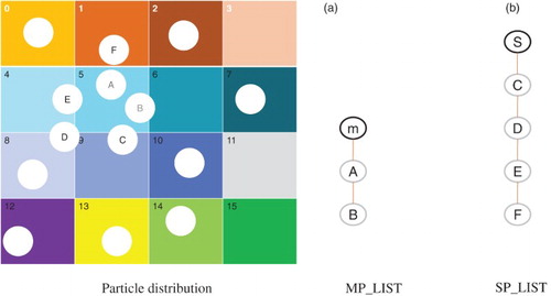
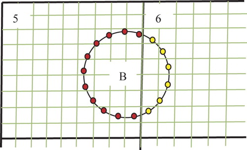
Figure 2. Schematic diagram of the Lagrangian points (marked in yellow) on which the interpolated fluid velocities in the SP_LIST of sub-domain 6 are sent to the MP_LIST of sub-domain 5.

The key of our algorithm is to establish two particle lists for each sub-domain: a main list (MP_LIST) and a subordinate list (SP_LIST). The main list is used to update the particle data in simulations and the subordinate list for the data communication in mutual interpolations. The MP_LIST contains the data of particles whose central positions are located in the sub-domain considered, and the SP_LIST stores the information of particles whose central positions are not located in the current sub-domain but whose pseudo body-forces have influence on (or are affected by) the velocities in the sub-domain due to the mutual interpolations. For sub-domain 5 in Figure 2, as an example, particles A and B belong to MP_LIST because of their central positions located in sub-domain 5. The particles C, D, E, and F belong to SP_LIST. Note that particle F belongs to SP_LIST because we assume that the gap distance between the particle and the boundary of sub-domain 5 is smaller than the size of one mesh (h), and thus its pseudo body-force affects (or is affected by) the velocity in sub-domain 5 (or on the boundary of sub-domain 5) via the interpolation, although none of the particle domain overlaps with sub-domain 5. The critical gap distance to determine whether particle F belongs to SP_LIST depends on the type of interpolation function (or discrete delta function), and is equal to the mesh size h for the tri-linear function we employed. Particle F is detected by the processor of sub-domain 1 as a member of its MP_LIST and a member of the SP_LIST of sub-domain 5, according to the particle position. Sub-domain 5 finds this particle by receiving the information from sub-domain nbsp;1.

For both MP_LIST and SP_LIST, we establish a new data structure to store the information of particles, including the particle sequence number, position, translational and angular velocities, pseudo body-force and fluid velocity defined on the Lagrangian nodes. For a particle in SP_LIST of each sub-domain, the fluid velocities on the Lagrangian nodes are computed from the interpolation of the velocities on the Eulerian points in the local sub-domain, and thus only the values at some of the Lagrangian points are obtained (e.g., the yellow Lagrangian points of particle B in sub-domain 6 in Figure 2). For particle B in Figure 2, these fluid velocities at the yellow Lagrangian points in the SP_LIST of sub-domain 6 are just needed by the MP_LIST of sub-domain 5 for a complete set of data. In order to transfer the data in the SP_LIST in a sub-domain to the MP_LIST in a neighboring sub-domain, we establish an index list for SP_LIST, whose contents include the sequence number of the sub-domain in which the particle center is located (i.e., identifying the MP_LIST), the index (sequence number) of the particle in the identified MP_LIST, and the flags of Lagrangian nodes (being 1 if the fluid velocity at this Lagrangian node is computed in this sub-domain, otherwise 0).

The full algorithm of our parallel FD method is the following:

1. Code initialization, including the construction of the MP_LIST for each sub-domain with a new data structure.

2. Establish the SP_LIST (as well as the index list) by exchanging the particle data in the MP_LIST among sub-domains. For a particle in the MP_LIST of one sub-domain, the particle data will be sent to the neighboring sub-domain if it is judged to belong to the SP_LIST of the neighboring sub-domain from the distance between the particle surface and the boundary of the neighboring sub-domain for the spherical particle considered.

3. Distribute the pseudo body-force from the Lagrangian points to the Eulerian nodes for both the MP_LIST and SP_LIST for each local sub-domain. No data communication is needed.

4. Solve the fluid sub-problem Equation (8–10) with the parallel multi-grid method mentioned earlier.

5. Compute the fluid velocity u* on the Lagrangian points in Equations (11–13) from the interpolation of the fluid velocities on the Eulerian nodes for the MP_LIST and SP_LIST of each sub-domain (as well as the flags of the Lagrangian points in the index list), and then send the data in the SP_LIST to the MP_LIST of the neighboring sub-domains with the index list, as described earlier.

6. Calculate the translational velocity Uⁿ⁺¹, angular velocity and pseudo body-force of the particle in the MP_LIST for each sub-domain from Equations (11–13).

7. Correct the fluid velocity uⁿ⁺¹ from Equation (14). The manipulation is the same as in step (3).

8. Deal with the collision of the particles with the collision model described below, if needed – otherwise, directly update the particle positions in the MP_LIST with the velocities obtained.

9. Update the MP_LIST. When the particle's central position changes from one sub-domain to another sub-domain, the particle is added to the MP_LIST of the new sub-domain and deleted from the MP_LIST of the old sub-domain.

10. Delete the SP_LIST and the index list, and go back to step (2) for the next time-step.

A flowchart for our parallel FD method, corresponding to the above algorithms, is presented in Figure 3.

Figure 3. Flowchart for the parallel FD method.

2.3.3. Parallel implementation strategy for collision model

Next, we describe our parallel algorithm for particle collision. The soft-sphere collision model is chosen, and the artificial repulsive force is given as (15) where F₀ is a constant, d is the particle inter-distance, is a cut-off distance, and is a unit vector of the particle connector. The procedure for our collision model is as follows:

1. Establish a particle list SP_LIST_C for each sub-domain by gathering the particle data in the MP_LIST of the neighboring sub-domains.

2. Seek the particle pairs satisfying the collision criterion by considering the relative positions (or possibly velocities for the hard-sphere model) of the particles in the MP_LIST with respect to other particles in the MP_LIST (same sub-domain), in the SP_LIST_C (neighboring sub-domains) and the wall boundaries.

3. Calculate the repulsive forces for the detected particle pairs and sum up to obtain the forces on the particles in the MP_LIST.

4. Update the velocities and positions of the particles in the MP_LIST in response to the repulsive forces.

In addition, we use a small time-step (normally one tenth of that for the solution of flow fields) for the collision model in order to improve the stability of the explicit scheme for the repulsive force (Glowinski et al., 1999).

3. Scalability of the parallel code

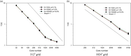
We choose two cases of particle-laden flows with grid numbers of 512³ and 1024³ to test the parallel efficiency of our FD code. The particle numbers are 1024, 10,240, and 102,400, respectively, corresponding to the volume fractions of 0.1%, 1% and 10%. One particle diameter covers 6.4 grids for the 512³ grid case and 12.8 grids for the 1024³ grid case. The tests were performed on the Yellowstone supercomputer at the National Center for Atmospheric Research. We ran one case for several time-steps and a few times, and then calculated the mean computational (wall-clock) time per one time-step. The particle collision and data input/output (IO) were not considered, since we focused on the parallel efficiency of our FD scheme. The particles were initially distributed randomly and homogeneously over the domain. Figure 4 shows the computational time for one time-step as a function of core (or processor) number. In Figure 4(a), we observe that for the case of 512³ the computational time is roughly reduced by half when the core number is doubled for the core number up to 1024, which corresponds to the grid number per core of 64 × 64 × 32. In other words, the parallel efficiency of our FD code is almost 100%, when the grid number per core does not exceed 64 × 64 × 32, above which the efficiency drops due to the increased data communication time relative to the computation time. In addition, Figure 4 shows that the effect of the particle number on the computational time is insignificant for three cases of particle numbers tested; the computational time caused by the presence of the particles is around 10% of the total computational time for the case of 102,400 particles. Figure 4(b) shows that for the case of 1024³ grid resolution, the speed-up of our parallel code remains largely linear, as the core number is increased up to 8192 (64 × 64 × 32 grid number per core).

Figure 4. Computational (wall-clock) times per one time-step for the particle-laden flows.

4. Application example

As mentioned earlier, our parallel FD method differs from our serial FD method only in the solvers for the pressure Poisson equation and the velocity Helmholtz equation. Some tests (such as particle sedimentation and particle inertial migration) show that both versions of our FD method produce almost the same results. Since our serial FD code has been validated in previous studies (Yu & Shao, 2007, 2010), the validations of our new parallel code are not shown here. We apply the new code to the investigation of the particle inertial effects on the turbulent channel flow. Our method is characterized by using the direct numerical simulation methods for both particle-laden and turbulent flows. Such methods have been applied to the simulations of particle-laden isotropic turbulent flows (Gao, Li, & Wang, 2013; Lucci, Ferrante, & Elghobashi, 2010; Ten Cate, Derksen, Portela, & Van den Akker, 2004) and turbulent channel flows (Do-Quang, Amberg, Brethouwer, & Johansson, 2014; Kidanemariam, Chan-Braun, Doychev, & Uhlmann, 2013; Pan & Banerjee, 1997; Shao et al., 2012; Uhlmann, 2008), but not for the effects of the particle inertia (i.e., particle-fluid density ratio) on the turbulent channel flow. In the following, we introduce the numerical model for the problem of interest, validate the accuracy for the single-phase case, conduct the mesh-convergence test for the particle-laden case, and finally report the main results.

4.1. Numerical model

Figure 5 shows the geometrical model of our particle-laden channel flow. Periodic boundary conditions are imposed in the streamwise and spanwise directions, and a non-slip wall boundary condition in the transverse direction. Let x, y and z represent respectively the streamwise, transverse and spanwise directions, a the particle radius, and H half of channel height in the transverse direction. We choose H and wall friction velocity as the characteristic length and velocity for the non-dimensionlization scheme. The wall friction velocity is defined by the wall shear stress and the fluid viscosity : . The friction Reynolds number is defined by . Because of the periodic boundary condition in the streamwise direction, a constant pressure gradient is needed to overcome the wall friction drag and sustain the flow. The value of the constant pressure gradient is , corresponding to the dimensionless value of .

Figure 5. Schematic diagram of the particle-laden channel flow.

The friction Reynolds number is 180. To study the effects of the particle inertia on the turbulent channel flow, different particle-fluid density ratios of are considered, and the gravity effect is ignored. The particle radius is . The size of our computational domain is . A uniform grid is employed and the grid number is . The particle volume fraction is 0.84%, corresponding to the particle number of . The dimensionless time-step is 0.0001 for and 0.0002 for the other cases.

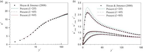
4.2. Validation for the single-phase case

In Figure 6, our results on the mean and root-mean-square (RMS) velocities of the particle-free turbulent channel flow are compared to those of Hoyas and Jimenez (2008), who employed the pseudo-spectral method. It can be seen that our results for the case of L = 8H (i.e., the computational domain size being ) agree well with those of Hoyas and Jimenez. For the low-friction Reynolds number of 180 considered, the sizes of and appear too small to produce size-independent results. This is the reason why we chose the computational domain size of .

Figure 6. Comparisons of mean and RMS velocities of the particle-free turbulent channel flow.

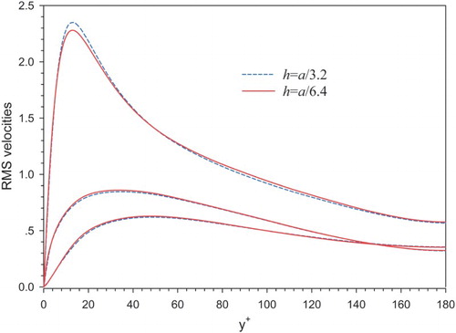
4.3. Mesh-convergence test for the particle-laden case

For the turbulent particle-laden channel flows, no benchmark data are available to validate the accuracy and, to our knowledge, no mesh-convergence tests have been performed, presumably due to high computational cost. For our simulation case of , there are only 3.2 meshes per particle radius, and one may question whether such mesh resolution is high enough to ensure acceptable accuracy. With the parallel code, it is now possible for us to conduct a mesh-convergence test. The parameters for the test case are and . The reason why we chose this density ratio is that the RMS velocities for deviate significantly from those for the particle-free case. For mesh h = a/3.2, the grid number is and the time-step is 0.0001, whereas for mesh h = a/6.2, the grid number is and the time-step is 0.00005, which is required by the stability condition due to mesh refinement. The results on the RMS velocities for two meshes are plotted in Figure 7. We observe a good agreement between the two results. The maximum relative error at the peaks of the streamwise RMS velocities is around 3% (2.35 vs 2.28) in Figure 7.

Figure 7. RMS velocities of the particle-laden turbulent channel flow obtained with two meshes of h = a/3.2 and h = a/6.4 in the case of .

4.4. Results and discussion

Figure 8 shows the mean velocity profiles for all cases studied. One can see that the flow flux first reduces and then increases, as the density ratio increases. Since the pressure gradient is fixed, a reduction in flow flux means an increase in flow resistance.

Figure 8. Mean velocity profiles for particle-free and particle-laden turbulent channel flows.

Figure 9 shows the RMS velocities in three directions. Generally, the presence of particles enhances the RMS velocities near the wall (very close to the wall for the streamwise component and not clearly shown in Figure 9) and attenuates the RMS velocities at the region away from the wall. The suppression of the RMS velocities at the bulk region becomes more pronounced for larger density ratios.

Figure 9. RMS velocities in the (a) streamwise, (b) transverse, and (c) spanwise directions for particle-free and particle-laden turbulent channel flows.

Figure 10 shows the vortex structures for the single-phase case and the density ratios of 10.42 and 104.2. The presence of particles weakens the large-scale vortices, and the effect is enhanced as the density ratio increases. A significant suppression of the large-scale vortices is found at ρ_r = 104.2, which is clearly responsible for the considerable attenuation of the RMS velocities at ρ_r = 104.2 in Figure 9. The presence of particles causes additional viscous dissipation (Lucci et al., 2010), which has dual effects on the flow drag. On one hand, more viscous dissipation means higher viscosity of the suspension and thereby larger flow drag. On the other hand, more viscous dissipation leads to suppression of the large-scale quasi-streamwise vortices which are primarily responsible for the drag-enhancement of turbulence with respect to laminar flow, and thereby lower flow resistance. The competition of these two effects gives rise to the results observed earlier: the flow drag first increases and then decreases with increasing density ratio.

Figure 10. Vortex structures for (a) the single-phase case, (b) , and (c) .

5. Conclusions

We have presented a parallel direct-forcing fictitious domain (DF/FD) method for the simulation of particulate flows and demonstrated its high parallel efficiency. The new code has been applied to studying the effects of particle inertia on the turbulent channel flow. The results show that the large-scale vortices are weakened more severely, and the flow friction drag increases first and then reduces, as particle inertia increases. We conjecture that the competition of the dual effects of particle-induced viscous dissipation on the flow drag is responsible for the variation of the flow drag with particle inertia. Our results on the particle inertial effects in the present study are preliminary, and we plan to conduct a more extensive study in the future.

References

- Balachandar, S., & Eaton, J. K. (2010). Turbulent dispersed multiphase flow. Annual Review of Fluid Mechanics, 42, 111–133. doi: 10.1146/annurev.fluid.010908.165243
- Blasco, J., Calzada, M. C., & Marin, M. (2009). A fictitious domain, parallel numerical method for rigid particulate flows. Journal of Computational Physics, 228, 7596–7613. doi: 10.1016/j.jcp.2009.07.010
- Borazjani, I., Ge, L., Le, T., & Sotiropoulos, F. (2013). A parallel overset-curvilinear-immersed boundary framework for simulating complex 3D incompressible flows. Computers & Fluids, 77, 76–96. doi: 10.1016/j.compfluid.2013.02.017
- Clausen, J. R., Reasor, D. A.Jr. & Aidun, C. K. (2010). Parallel performance of a lattice-Boltzmann/finite element cellular blood flow solver on the IBM Blue Gene/P architecture. Computer Physics Communications, 181, 1013–1020. doi: 10.1016/j.cpc.2010.02.005
- Do-Quang, M., Amberg, G., Brethouwer, G., & Johansson, A. V. (2014). Simulation of finite-size fibers in turbulent channel flows. Physical Review E, 89, 013006. doi: 10.1103/PhysRevE.89.013006
- Gao, H., Li, H., & Wang, L. P. (2013). Lattice Boltzmann simulation of turbulent flow laden with finite-size particles. Computers & Mathematics with Applications, 65, 194–210. doi: 10.1016/j.camwa.2011.06.028
- Glowinski, R., Pan, T. W., Hesla, T. I., & Joseph, D. D. (1999). A distributed Lagrange multiplier/fictitious domain method for particulate flows. International Journal of Multiphase Flow, 25, 755–794. doi: 10.1016/S0301-9322(98)00048-2
- Hoyas, S., & Jimenez, J. (2008). Reynolds number effects on the Reynolds-stress budgets in turbulent channels. Physics of Fluids, 20, 101511. doi: 10.1063/1.3005862
- Hu, H. H., Patankar, A., & Zhu, M. Y. (2001). Direct numerical simulations of fluid-solid systems using the arbitrary Lagrangian-Eulerian technique. Journal of Computational Physics, 169, 427–462. doi: 10.1006/jcph.2000.6592
- Kidanemariam, A. G., Chan-Braun, C., Doychev, T., & Uhlmann, M. (2013). Direct numerical simulation of horizontal open channel flow with finite-size, heavy particles at low solid volume fraction. New Journal of Physics, 15, 025031. doi: 10.1088/1367-2630/15/2/025031
- Ladd, A. J. C. (1994). Numerical simulations of particulate suspensions via a discretized Boltzmann equation. Part 1.Theoretical foundation. Journal of Fluid Mechanics, 271, 285–309. doi: 10.1017/S0022112094001771
- Lucci, F., Ferrante, A., & Elghobashi, S. (2010). Modulation of isotropic turbulence by particles of Taylor length-scale size. Journal of Fluid Mechanics, 650, 5–55. doi: 10.1017/S0022112009994022
- Pan, Y., & Banerjee, S. (1997). Numerical investigation of the effects of large particles on wall turbulence. Physics of Fluids, 9, 3786–3807. doi: 10.1063/1.869514
- Shao, X. M., Wu, T. H., & Yu, Z. S. (2012). Fully resolved numerical simulation of particle-laden turbulent flow in a horizontal channel at a low Reynolds number. Journal of Fluid Mechanics, 693, 319–344. doi: 10.1017/jfm.2011.533
- Shao, X. M., Yu, Z. S., & Sun, B. (2008). Inertial migration of spherical particles in circular Poiseuille flow at moderately high Reynolds numbers. Physics of Fluids, 20, 103307. doi: 10.1063/1.3005427
- Tai, C. H., Zhao, Y., & Liew, K. M. (2005). Parallel computation of unsteady incompressible viscous flows around moving rigid bodies using an immersed object method with overlapping grids. Journal of Computational Physics, 207, 151–172. doi: 10.1016/j.jcp.2005.01.011
- Ten Cate, A., Derksen, J. J., Portela, L. M., & Van den Akker, H. E. A. (2004). Fully resolved simulations of colliding monodisperse spheres in forced isotropic turbulence. Journal of Fluid Mechanics, 519, 233–271. doi: 10.1017/S0022112004001326
- Tryggvason, G. (2010). Virtual motion of real particles. Journal of Fluid Mechanics, 650, 1–4. doi: 10.1017/S0022112010000765
- Uhlmann, M. (2003). Simulation of particulate flows on multi-processor machines with distributed memory. CIEMAT Technical Report No. 1039, Madrid, Spain.
- Uhlmann, M. (2005). An immersed boundary method with direct forcing for the simulation of particulate flows. Journal of Computational Physics, 209, 448–476. doi: 10.1016/j.jcp.2005.03.017
- Uhlmann, M. (2008). Interface-resolved direct numerical simulation of vertical particulate channel flow in the turbulent regime. Physics of Fluids, 20, 053305. doi: 10.1063/1.2912459
- Wang, S., He, G., & Zhang, X. (2013). Parallel computing strategy for a flow solver based on immersed boundary method and discrete stream-function formulation. Computers & Fluids, 88, 210–224. doi: 10.1016/j.compfluid.2013.09.001
- Wang, Z. L., Fan, J. R., & Luo, K. (2008). Parallel computing strategy for the simulation of particulate flows with immersed boundary method. Science in China Series E: Technological Sciences, 51, 1169–1176. doi: 10.1007/s11431-008-0144-3
- Wesseling, P. (1992). An introduction to multigrid methods. New York, US: John Wiley & Sons.
- Yildirim, B., Lin, S., Mathur, S., & Murthy, J. Y. (2013). A parallel implementation of fluid–solid interaction solver using an immersed boundary method. Computers & Fluids, 86, 251–274. doi: 10.1016/j.compfluid.2013.06.032
- Yu, Z. S., Phan-Thien, N., & Tanner, R. I. (2004). Dynamical simulation of sphere motion in a vertical tube. Journal of Fluid Mechanics, 518, 61–93. doi: 10.1017/S0022112004000771
- Yu, Z. S., & Shao, X. M. (2007). A direct-forcing fictitious domain method for particulate flows. Journal of Computational Physics, 227, 292–314. doi: 10.1016/j.jcp.2007.07.027
- Yu, Z. S., & Shao, X. M. (2010). Direct numerical simulation of particulate flows with a fictitious domain method. International Journal of Multiphase Flow, 36, 127–134. doi: 10.1016/j.ijmultiphaseflow.2009.10.001
- Yu, Z. S., Shao, X. M., & Wachs, A. (2006). A fictitious domain method for particulate flows with heat transfer. Journal of Computational Physics, 217, 424–452. doi: 10.1016/j.jcp.2006.01.016