Numerical simulations of flow pattern and particle trajectories in feline aorta for hypertrophic cardiomyopathy heart conditions

ABSTRACT

Numerical simulations of pulsatile flow in a feline aorta for hypertrophic cardiomyopathy (HCM) heart conditions are performed to predict flow details and to evaluate possible thrombus trajectory patterns. The study demonstrates that average flow rate boundary conditions (Q_BC) at artery outlets act as a resistance-type boundary condition for pulsatile flow. For simulations when the exact artery outflows are not known, specification of estimated values from physiological conditions is a plausible approach. This boundary condition is further improved using an iterative method (I-Q_BC) to accurately satisfy outflow conditions when expected outflow is known. The approach is validated against experimental data for the prediction of iliac artery flow and wall stresses in a human abdominal aorta. The feline aorta simulations including Lagrangian particle transport are performed on grids with up to 11M cells for a generalized feline aorta. It is found that LES on larger grids performs significantly better than URANS for the prediction of vortical structures. Simulations for both healthy and HCM conditions show similar flow patterns in the upper abdominal aorta. However, the HCM condition shows the presence of large recirculation regions in the thoracic aorta resulting in 50% lower flow through the iliac arteries and increased entrapment of fluid-borne particles near the trifurcation region compared to the healthy condition.

KEYWORDS:

• Hypertrophic cardiomyopathy (HCM)
• feline aorta
• computational fluid dynamics (CFD)
• turbulence modeling
• particle transport

1. Introduction

Hypertrophic cardiomyopathy (HCM) is one of the most common inherited cardiac diseases among humans and affects about 1 in 500 individuals. HCM is also a very common disease in felines even in clinically healthy cats (Kittleson et al., 1999; Maron & Maron, 2013). HCM is caused by the thickening of the left ventricular muscle wall, which results in decreased relaxation and increased diastolic pressure in the left ventricle and increased stasis of blood in the left atrium. This affects the aortic flow and results in formation of blood clots (thrombi) in the left atrium (Ferasin, 2009; Maron et al., 1985). Free thrombi are transported along with the blood, and depending upon the complex interplay of various factors such as blood flow conditions (vorticity, shear, turbulence etc.), size of thrombi, roughness of blood vessel/endothelium, hypercoagulability, and endothelial injury (Pasipoularides, 2011), thrombi may attach to the blood vessel wall (thrombogenesis) with the long-term potential of partially or completely occluding blood flow in the aorta. The pathophysiology of thrombogenesis is not well understood and is a subject of ongoing research.

Computational fluid dynamics (CFD) has been widely used to investigate blood flow physiology and to design cardiovascular devices (Bhushan, Walters, & Burgreen, 2013) and can potentially assist in understanding the pathophysiology of thrombogenesis associated with HCM. Two non-trivial challenges for CFD simulations are the specification of artery outlet boundary conditions for pulsatile flow to mimic the truncated arterial network, and accurate prediction of the thrombotic cascade (Sorensen, Burgreen, Wagner, & Antaki, 1999).

A review of the literature shows that most pulsatile aortic flow simulations use atmospheric pressure boundary conditions at artery outlets. For example,¹ Karmonik, Bismuth, Davies, and Lumsden (2008) performed simulations for patient-specific human aorta geometry and cardiac flow conditions. The flow, pressure and wall shear stress distribution on the aorta wall were analyzed to identify the potential for aortic thrombogenesis. McGarry, Hitt, and Harris (2008) performed simulations in an idealized artery geometry with puncture, and time-averaged local strain rates near the artery puncture were examined to study the physiological implications of hemostasis. Khanafer and Berguer (2009) studied the effect of pulsatile cardiac flow on the aortic wall stresses (and deformation) using fluid-structure interaction. Gardhagen, Carlsson, and Karlsson (2015) performed simulations in idealized aorta models with coarctation and post stenotic dilatation, and flow turbulence and associated stresses were analyzed to estimate the hemodynamic risks. Deep (2013) specified a constant pressure at the boundary that was obtained from (averaged) uniform flow simulations. The approach was used for simulations of flow through healthy and diseased patient aorta models, and the wall stress distribution was correlated to atherosclerosis.

In contrast to the constant pressure boundary condition, some studies have specified cardiac cycle averaged expected flow rate at artery outlets (in terms of % of inlet flow). We denote such an approach here as Q_BC. For example, Howell et al. (2007) performed simulations for a patient-specific abdominal aortic geometry and specified inflow conditions to assess the hemodynamic forces acting on a bifurcated abdominal stent-graft. Benim et al. (2011) performed simulations for flow through a human aorta and its major branches for specific physiologic conditions. The study also proposed a resistance-type boundary condition for scenarios when the expected artery outflows were not available. It was argued that the flow distribution between the aortic branches could change depending on the circulation type; however, the flow resistance caused by the anatomy of the downstream vasculature does not change. The flow-resistance coefficients were estimated from the averaged outlet pressure and flow rate predicted in the physiological condition simulations. The method was applied for extracorporeal circulation with (averaged) uniform inflow, and the flow and wall stress pattern were analyzed to study the mobilization of arteriosclerotic plaques.

Huo, Guo, and Kassab (2008) specified pressure waveforms at the aorta outlets obtained from in-vivo measurements. The approach was applied for flow in a mouse aorta, wherein the variations of wall stresses over the cardiac cycle were used to study the physiology. Taylor, Hughes, and Zarins (1999) used the Womersley approach to specify the outflow pressure waveform due to atherosclerosis for idealized human abdominal aorta simulations. The flow path lines and velocities, wall shear stresses, dynamic pressures and flow residence times were analyzed to identify possible sites of aortic thrombogenesis. In the Womersley approach, an analytic solution for the outflow pressure waveform is derived assuming a pulsatile Poiseuille flow between the inlet and outlet (Womersley, 1957). Advanced variants of the Womersley approach have also been proposed, such as the resistance-capacitance-type model proposed by Olufsen (1999). Cheema et al. (2014), for example, used such a model to study the deformation characteristics of a porous aortic arch using fluid-structure interaction.

Overall, a constant pressure boundary condition is deficient for pulsatile flow simulations and fails to yield accurate resolution of the wall stresses and pressure (Cheema et al., 2014; Khanafer & Berguer, 2009). The most theoretically accurate approach is the specification of the outlet pressure waveform obtained from in-vivo measurements, but that method cannot be used for exploratory studies. Methods based on a derived pressure waveform have similar difficulties, as they require knowledge of the inflow pressure waveform. The Q_BC approach provides a simple alternative, which justifies its investigation as a viable method. In the current study, it is demonstrated that such a boundary condition acts as a resistance-type, i.e. the specified flow rate is the expected value that the downstream vasculature seeks to draw from the aorta, and the expected value remains unchanged irrespective of the cardiac output or the aorta shape, following the argument of Benim et al. (2011).

Most of the studies available in the literature have used flow properties and wall stresses to evaluate the physiology of aortic thrombogenesis, arteriosclerosis, etc. Few blood flow studies include particle transport, even though it is quite common for lung airway simulations (e.g. Walters & Luke, 2011). One possible reason for this is the scale gap between the fluid (of the order of nanometers) and the thrombi (of the order of micrometers) for such flows. Hence, the dynamics of the particles and their interaction with the wall is strongly dependent on their deformation and thermal fluctuations, which often occurs in the non-Newtonian regime and cannot be accurately predicted by the particle-transport simulations for continuum fluid flow (Fedosov, Noguchi, & Gompper, 2014). Other reasons include the fact that thrombi transport in circulation is a much less common event than particle inhalation into lungs, and the difficulties in obtaining reliable experimental data for thrombus tracking and deposition in opaque blood.

The objectives of this study are to perform simulations of pulsatile feline aortic flow with Lagrangian thrombus transport for HCM heart conditions, to understand the effect of cardiac outflow changes on the aortic and abdominal artery flows, and to investigate the effect of HCM on the probability of thrombogenesis. The study demonstrates that Q_BC is a plausible artery outflow boundary condition for pulsatile flow when the exact time-dependent artery flow rate is not known. In addition, an iterative method is developed to improve Q_BC to exactly satisfy artery outflow, when the expected time-averaged flow rate is known. The simulations are performed for a generalized feline aorta model for healthy and HCM conditions, including grid verification and turbulence modeling studies. The linkage between the probabilities of thrombogenesis as related to potential thrombi trajectories through the aorta and the roles of aortic flow in the entrapment of thrombi are discussed.

2. Computational models and methods

The simulations are performed using the commercial flow solver ANSYS/Fluent® version 14.0 (FLUENT, 2006). ANSYS/Fluent was chosen because it is a well-validated CFD solver with a very large validation base available in the open literature. The software also includes a wide selection of numerical methods and turbulence modeling options relevant to the current study. The authors have previously validated the solver for a wide range of laminar and turbulent flows in wall-bound and free-shear regimes, including rigorous verification of numerical schemes and subgrid stress models for large-eddy simulation (Adedoyin, Walters, & Bhushan, 2015), and biomedical applications such as lung airway (Walters, Burgreen, Lavallee, Thompson, & Hester, 2011) and cardiovascular device flows (Bhushan et al., 2013).

The blood flow is assumed to be Newtonian and governed by the incompressible Navier-Stokes equations. Unsteady Reynolds-averaged Navier-Stokes (URANS) simulations are performed using the - shear stress transport (SST) model (Menter, 1994). SST is a well-validated URANS model for engineering accurate CFD simulation, and has been successfully demonstrated in the open literature for a wide range of applications, including aorta flows similar to those performed in this study (Benim et al., 2011). Large eddy simulations (LES) are performed using the monotonically integrated LES (MILES) approach as recommended by Adedoyin et al. (2015) for Fluent simulations. MILES does not include any explicit turbulence modeling, rather it assumes numerical dissipation of the same order magnitude as LES stresses. In general, MILES is not expected to be as accurate as explicit models for near-wall turbulence predictions. For the current simulations, however, Reynolds numbers are sufficiently low than universal high-Re turbulent boundary layer characteristics – such as the high turbulence production in the buffer layer and equilibrium log-layer regions – are not expected to be present. The appropriateness of the MILES approach in the near-wall region is validated by comparison of predicted wall shear stress distribution with experimental data.

Particle transport simulations are performed using the coupled discrete phase and discrete element models available in Fluent. The particles are considered neutrally buoyant inert particles transported by the fluid. The inertia of the particles and the effect of Brownian motion are neglected as this study primarily focuses on the prediction of idealized particle trajectories and particle accumulation in the aorta based on the residence time of the carrier fluid (blood) during the cardiac cycle.

Transient simulations are performed using the pressure-based solver option, which is the typical predictor-corrector method, and requires solution of pressure via a Poisson equation to satisfy mass conservation. Pressure-velocity coupling uses the Pressure-Implicit with Splitting of Operators (PISO) scheme. Unsteady terms are discretized using a second order implicit (three-point backward difference) scheme. The convective terms in the momentum equations are discretized using a second order upwind linear reconstruction scheme for URANS simulations and the Bounded Central Difference (BCD) scheme for LES as recommended by Adedoyin et al. (2015). The particle transport equations are solved using implicit Euler integration.

3. Simulation setup and conditions

3.1. Geometries and grids

A computer-aided design (CAD) model of the human abdominal aorta geometry is generated using dimensions reported in the experimental setup (Moore, Ku, Zarins, & Glagov, 1992) (Figure 1). The aortic geometry includes the major circulation structures: celiac artery, cranial mesenteric artery (CrMA), right and left renal arteries, caudal mesenteric artery (CuMA), and right and left iliac arteries. The total length of the aorta from the inlet to the bifurcation is 180 mm. An unstructured tetrahedral mesh consisting of 2.5M cells is generated for which the average wall distance of the first grid point away from the wall is y⁺ < 0.5. Note that the average y⁺ is estimated for the peak aortic flow when the Reynolds number is expected to be highest.

Figure 1. Human abdominal aorta domain and grid. Inset figure shows the mesh resolution at the inlet surface, and CuMA and iliac bifurcations.

The feline aorta model (Figure 2) consists of an ascending aorta, which starts from the left ventricle, an arch section that leads to the thoracic aorta and later becomes the abdominal aorta, and terminates in a trifurcation. The major arteries considered for the feline aorta are: brachiocephalic trunk, left subclavian artery, celiac artery, CrMA, right and left renal arteries, CuMA, and right, left and common iliac arteries. The CAD model is generated using the dimensions of the feline aorta of Samii, Biller, and Koblik (1998), and any missing information is estimated by scaling the dimensions of the human aorta (Moore et al., 1992). Details of the aorta geometry and dimensions are summarized in Table 1. Initially, a coarse grid consisting of 1.5M tetrahedral cells with averaged y⁺ ∼ 2 is generated, then adaptively refined using a grid refinement ratio r_G = √2 to obtain grids with 4.2M cells (medium) and 11M (fine) cells with averaged y⁺ = 1.2 and 0.9, respectively.

Figure 2. Feline aorta domain and grid shown for the finest grid with 11M cells. Inset figure shows mesh resolution at the inlet, CuMA bifurcation and iliac trifurcation, and major and minor axis of the brachiocephalic artery.

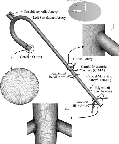
Table 1. Feline aorta geometry details, expected and predicted % mass flow from arteries, and number of particles escaping from the arteries in healthy and HCM conditions.

					Healthy condition			HCM condition
					I-QBC
Artery	Length/Location	Diameter (mm)	Branching angle	Target Q%	Prescribed Q		% Particle escaped	Predicted	% Change*	% Particle escaped
Cardiac Aorta	–	5.35	–	–	–	–	–	–	–	–
Brachiocephalic	1.5 cm above Thoracic	5.09 (major axis),Table 13.03(minor axis)^£	∼90°	31.65%	33.81%	0.57%	53.40%	41.01%	21.30	45.23%
Left Subclavian	1.5 cm above Thoracic	2.8 (major axis),1.74(minor axis)	∼90°	7.91%	8.45%	0.27%	7.59%	11.08%	31.12	13.69%
Celiac	4.39 cm from Trifurcation	1.456	55.7°	12.69%	11.03%	0.002%	7.39%	11.74%	6.44	6.05%
Cranial Mesenteric (CrMA)	3.870 cm from Trifurcation	1.421	61.1°	9.07%	8.24%	0.14%	4.71%	7.32%	−11.17	5.04%
Right Renal	3.44 cm from Trifurcation	1.070	61.4°	9.07%	8.57%	0.002%	4.99%	8.79%	2.57	3.99%
Left Renal	3.307 cm from Trifurcation	1.035	65.3°	9.07%	8.57%	0.002%	5.62%	8.81%	2.80	4.76%
Caudal Mesenteric (CuMA)	1.367 cm from Trifurcation	0.579	41.1°	2.42%	2.20%	0.001%	1.49%	2.20%	0.00	1.39%
Right Iliac	Located at trifurcation	1.391	50.7°	6.04%	6.45%	0.07%	3.17%	2.86%	−55.66	1.33%
Left Iliac		1.391	50.7°	6.04%	6.45%	0.06%	3.63%	2.83%	−56.12	1.34%
Common Iliac		1.391	0°	6.04%	6.23%	0.02%	3.52%	3.59%	−42.38	1.38%
Total	–	–	–	–	–	–	95.52%	–	23%(Abs. Avg.)	84.21%

^§Difference between predicted and target Q.

*%Change is with respect to healthy condition mass flow predictions.

^£Major axis and minor axis are depicted in Figure 2.

3.2. Simulation conditions

Table 2 summarizes the eight cases performed in this study. In case 1, LES of human abdominal aorta flow is performed for healthy condition to evaluate appropriate artery outflow boundary conditions for pulsatile flows, including validation of the iterative target flow rate boundary condition (I-Q_BC). The results are validated using Moore et al. (1992) and Moore and Ku (1994) experiments and Taylor et al. (1999) CFD results. The simulation is performed using the inflow conditions and kinematic viscosity ν = 1 × 10⁻⁶ m²/s reported in the experiment. The Reynolds number (Re) of the flow based on the peak inlet velocity (U_p = 0.16 m/s) and aorta length is Re_L ∼2.9 × 10⁴, and that based on U_p and aorta diameter at the inlet is Re_D = 4500.

Table 2. Summary of simulation geometries, domains, grids, boundary conditions and objectives.

Case #	Geometry	Inlet(Cardiac output)	Grid Size(Million cells)	Turbulence Model	Artery outlet boundary	Objective
1	Human abdominal aorta	Healthy	2.5	LES	Outflow, Patm, Pconst, QBC, I-QBC	• Comparison of different artery outlet boundary conditions, and validation of I-QBC
						• Comparison with Taylor et al. (1999) results using Womersley boundary condition.
						• Validation using experimental data (Moore & Ku, 1994 Moore et al., 1992).
2	Feline aorta	Healthy	1.5, 4.2, 11	LES	I-QBC	• Grid study
3			4.2	LES		• Analysis of overall flow variation over a cardiac cycle
4			11	URANS, LES		• Turbulence model study
						• Analysis of growth/decay of vortical structures
5	Feline aorta	HCM	4.2	LES	QBC	• Analysis of overall flow variation over a cardiac cycle
						• Comparison with healthy condition predictions (case 3)
6			11			• Analysis of growth/decay of vortical structures
						• Comparison with healthy condition predictions (case 4)
7	Feline aorta	Healthy w/ particle injection	11	LES	I-QBC	• Analysis of role of cardiac output and associated flow features on the thrombus trajectory.
8		HCM w/ particle injection			QBC

Cases 2–4 focus on feline aorta simulations for healthy conditions. In case 2, a grid verification study is performed to quantify the numerical uncertainty interval in the simulations using the adaptively refined grids. In case 3, the variation of flow, turbulence and wall stresses over the cardiac cycle are analyzed using the intermediate 4.2M grid results. In case 4, the effect of turbulence models on the flow and generation/decay of vortical structures are discussed using the finest 11M grid results. Cases 5 and 6 focus on feline aorta simulations for HCM conditions, corresponding in all other respects to the healthy condition cases 3 and 4, respectively. The healthy and HCM condition results are compared to understand the effect of cardiac outflow changes on the aortic and artery flows. Cases 7 and 8 are performed to study particle trajectories in the feline aorta for healthy and HCM conditions, respectively, using LES on the finest 11M cell grid. The instantaneous and cardiac cycle averaged results are analyzed to understand the effect of cardiac output and associated flow features on potential thrombus trajectory in the aorta.

The feline aorta simulations are performed using averaged ν = 3.3 × 10⁻⁶ m²/s expected for feline blood at a body temperature of 38°C (Lipowsky, Usami, & Chien, 1980). The expected maximum Reynolds number, based on the total aorta length of 15 cm and peak inlet velocity is Re_L = 5.46 × 10⁴. The diameter-based Reynolds number for the largest artery (brachiocephalic) is Re_D = 1.85 × 10³.

3.3. Boundary conditions

The simulations require boundary conditions at the inlet, artery outlets, and on the aorta surface. The inlet and artery outlet boundary conditions are discussed below. The aorta wall is assumed to be rigid, and a no-slip boundary condition is used. A rigid wall is justified for the human aorta simulations since it is consistent with experiments used for validation, and with the previous numerical simulations (Taylor et al., 1999) used for comparison to the current results. Furthermore, while wall deformation modeling is expected to have significant effect on the wall stress predictions, it has been found to have a relatively small effect on the velocity field and flow distribution (Perktold & Rappitsch, 1995). Since the primary focus of the study is on the development of an appropriate outflow boundary condition at artery outlets and flow distribution predictions, a rigid wall is deemed to be reasonably accurate.

Inlet. The velocity profile for the human abdominal aorta simulation (Figure 3a) is extracted from the data of Taylor et al. (1999), which were based on the experiments of Moore et al. (1992). The velocity profile is applied as a time-periodic but spatially uniform inlet condition. Note that the use of a spatially uniform velocity at the inlet is physically incorrect as it does not account for the boundary layer. In the simulations, the flow adjusts just downstream of the inlet due to development of the boundary layer, and the peak velocity at the centerline increases by 3% over the prescribed inlet values, which is reasonably small.

Figure 3. Inlet velocity profile for (a) human abdominal aorta for healthy condition, and (b) feline aorta for healthy and HCM conditions over a cardiac cycle. (c) Time history of mass outflow from the feline common iliac artery for HCM condition over 15 cardiac cycles.

For feline aorta simulations, a pulsatile velocity profile for either healthy or HCM condition is applied at the inlet as shown in Figure 3b. Actual feline in-vivo cardiac output measurements are not available, therefore the velocity profiles are obtained by scaling the in-vivo human cardiac output measurements of Maron et al. (1985). The profiles are scaled to match the cardiac period and mass flow rate expected in cats (Johnston & Owen, 1977). The healthy condition shows a single peak pattern (systole) followed by diastole when there is no flow. The HCM condition shows a dual peak pattern, referred to as primary and secondary systole, followed by diastole. Note that the differences in the diastole velocity for the human abdominal and feline aorta cases are due to the difference in measurements, i.e. experimental setup for the former vs. in-vivo measurements for the latter.

For the healthy and HCM heart conditions, Maron et al. (1985) reported 4.5% and 9.5% variations in the peak flow and time measurements. The variations are expected due to both experimental uncertainty and turbulence generated from the aorta valve opening and closing. The experimental uncertainties were not reported. Therefore, it is assumed that half of the variation (or 2%) for the healthy conditions are due to turbulence. The HCM condition is expected to involve higher turbulence than healthy condition due to incomplete mitral valve closure, which is estimated to be around 5 to 7% based on the experimental variations. For LES, random phase fluctuations () are superimposed over the aorta velocity profiles to mimic the turbulence. For the healthy condition, nominal turbulence intensity TI = 2% (i.e. where u′ is the turbulent velocity fluctuation and U is the inlet velocity) is used, as estimated from the experiments. For HCM condition TI = 2%, 5% and 10% are used. It was found that the magnitude of the imposed turbulence intensity does not show significant effect on the flow. Thus, only the results using TI = 10% are reported in the study.

Artery Outflow. Fluent provides several outlet boundary condition options: Dirichlet pressure, Neuman pressure, outflow, and target mass flow rate. For the Dirichlet pressure boundary condition, static (gauge) pressure at the outlet is specified. For the Neumann pressure boundary condition, a zero pressure gradient boundary condition is used. The outflow boundary condition extrapolates the velocity and pressure at the outlet using the information from the interior. In Q_BC, a target mass flow rate as expected from an artery is specified (which is the same as specification of flow rate for incompressible flow, since density is constant). In this boundary condition, the artery outlet pressure is numerically adjusted (by a value ) at every time step (t + δt) as: (1) where is the flow rate at any instant and is the specified flow rate. For non-pulsatile flow, the above method converges when , which results in . However for pulsatile flows, is specified to be cardiac cycle averaged flow rate from the artery. For such flows, Eq. (1) is a differential equivalent of a resistance boundary condition proposed in Benim et al. (2011), wherein the left-hand side represents the pressure change between each time step for pulsatile flow, and the right-hand side is the flow resistance that depends on the expected averaged flow from the downstream vasculature. For simulations for which the expected flow rates from arteries () are known, the obvious choice for the boundary condition is ; however, as discussed in the next section, Eq. (1) fails to predict the required averaged flow rate over a cardiac cycle, i.e. (2) where T is the cardiac cycle period.

In this study, an iterative-targeted flow rate boundary condition (I-Q_BC) is developed to address the flow rate mismatch. In I-Q_BC, the specified averaged flow rate at the boundary () is varied for each successive cardiac cycle based on the error in the averaged flow rate prediction as below: (3) where the superscript (N) denotes the cardiac cycle iteration level, β is the relaxation factor for the iteration, which is specified to be 0.5, and is the error in the flow rate prediction calculated as: (4) The iteration is started with an initial guess . For both the human and feline aorta simulations under healthy conditions, I-Q_BC is used to estimate , which relates to the estimation of flow resistance coefficients. For HCM conditions, when exact values of are not known, the values obtained in healthy conditions are used. This is justified as a reasonable approximation since the flow-resistance from the downstream vasculature is expected to remain the same, while the actual average flow rate through each of the outlets is expected to vary (Benim et al., 2011).

3.4. Simulation parameters

The human abdominal aorta simulations are performed for 5 cardiac cycles, and feline aorta simulations for 10 to 15 cardiac cycles. Both sets of simulations use a fixed time-step size Δt = 0.0002 seconds, i.e. 4500 and 1500 time steps per cardiac cycle for human and feline aorta simulations, respectively. For each time step, 20 Newton (sub time step) iterations are used. In URANS, the residuals for the mass conservation dropped to <10⁻⁷ at the end each time-step, whereas in LES the residuals dropped to <10⁻⁶. The solutions are deemed converged when the artery outflow profiles do not show significant change between successive cardiac cycles. The variation of flow in the feline common iliac artery under HCM condition over 15 cardiac cycles is shown in Figure 3c. In most simulations, the convergence is achieved in a small number of cycles. However, for particle transport simulations the solutions are found to converge only after approximately eight cardiac cycles.

4. Results and discussion

4.1. Validation of human aorta predictions (Case 1)

Moore et al. (1992) performed experiments in a glass blown human aorta model constructed from cadaver specimens. Precision needle valves were used to control outflows from each artery, and a capacitance bottle was used at the iliac arteries to simulate the capacitance in the lower limbs. The mass flow rate waveforms at the iliac artery for resting and exercising conditions were measured, and the flow was visualized using dye injection. In a follow on study, Moore and Ku (1994) measured wall shear stress at supra-renal, infra-renal and bifurcation regions for the same flow conditions. Herein, iliac artery outflow waveform and shear stress profiles at the infra-renal region at peak systole under resting conditions are used for validation.

Figure 4a compares the iliac artery mass flow rate profile obtained using several different boundary conditions with the experimental data and Taylor et al. (1999) CFD results. The experimental data shows a peak flow coincident with the peak systole, a backflow at the end of systole, and an almost constant flow during diastole. The constant pressure and zero pressure gradient boundary conditions show similar results, but do not capture the peak or the backflow pattern. The outflow boundary condition predicts an iliac flow profile similar to the inlet profile, but with a lower amplitude.

Figure 4. (a) Mass outflow rates (kg/s) from the iliac artery during one cardiac cycle obtained using different artery outlet boundary conditions are compared with experimental data (Moore et al., 1992) and Taylor et al. (1999) results. (b) I-Q_BC convergence over 4 cardiac cycles (iterations 1–4) are shown by comparing predicted cardiac cycle averaged mass flow rate from arteries at every iteration with expected target values.

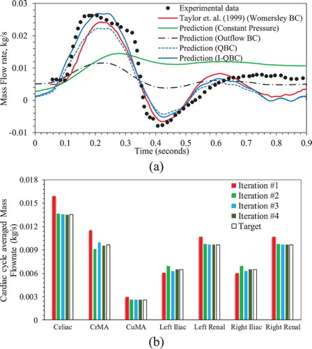
The Q_BC predictions show qualitatively good agreement with the experimental data, but approximately 18% error in the predicted average from the arteries, and approximately 21% error in the iliac profile, compared with experimental data. The I-Q_BC iteration converges within 4 to 5 iterations (cardiac cycles) as shown in Figure 4b, i.e. the artery outlet mass flow prediction error is reduced to . Most of the arteries such as celiac, CuMA, left renal, and right renal show monotonic convergence. However, arteries further downstream, such as CrMA, left and right iliac show oscillatory convergence. The I-Q_BC iliac predictions are quantitatively better than those obtained using Q_BC when compared with the experimental data, as both the peak and backflow magnitudes increase. The averaged error for the iliac profile is estimated to be 11.6%. The predictions are similar to those of Taylor et al. (1999) using a Womersley boundary condition, which show averaged error of 11.9%. I-Q_BC is somewhat more accurate than the Womersley boundary condition for the peak flow predictions, whereas the latter is better for the backflow predictions. In the diastole, both Q_BC, I-Q_BC and Womersley boundary condition predictions show a secondary peak around t = 0.6 s, followed by a trough at 0.8 s. The peaks and troughs are coincident with the inflow secondary peak and troughs (as observed in Figure 3a). The diastole flow dynamics in the simulations are different from that in the experiment, where the latter shows almost uniform flow rate.

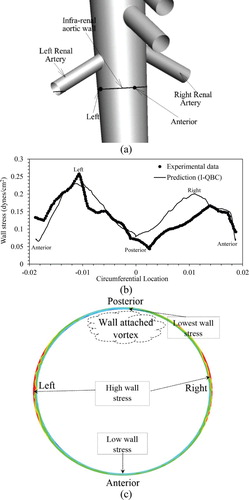
Shear stress predictions at the infra-renal wall (Figure 5a) are compared with experimental data in Figure 5b and show reasonable qualitative agreement. Both indicate maximal stresses reside on the right and left side of the aortic wall and minimal values on the anterior and posterior walls. Quantitatively, the predictions compare well with the experimental data between the anterior, left, and posterior walls, but show about 23% overprediction of stress between the posterior and right walls. Analysis shows that the high stresses on the left and right walls is due to accelerating flow below the renal artery branching, caused by high stagnation pressure at the renal-aorta bifurcation. The low stress of the posterior wall is identified to be due to flow stagnation caused by vortex formation, which is consistent with Taylor et al. (1999). The results in Figure 5b also demonstrate that the use of a MILES approach in the near-wall region does not lead to significant error in shear stress prediction, which is expected to be more sensitive to the details of the subgrid stress model than the bulk flow characteristics that are the focus of this study.

Figure 5. Validation of wall stress prediction for human abdominal aorta case. (a) Infra-renal aortic wall, and anterior and left wall locations are marked on the aorta geometry. (b) Wall shear stress (dynes/cm²) on infra-renal aortic wall at systole peak is compared with experimental data (Moore & Ku, 1994). (c) Wall stress contours on the infra-renal aortic wall; schematics point out high and low values.

4.2. Grid verification for feline aorta simulations (Case 2)

The numerical uncertainty (U_SN) in the simulations due to grid resolution is estimated using 2-Grid and 3-Grid methods, namely the grid convergence index (GCI), correction factor (CF) and factor of safety (FS) methods (Robertson, Choudhury, Bhushan, & Walters, 2015). The 2-Grid method is applied for coarse-medium (G23), coarse-fine (G13), and medium-fine (G12) grid pairs, whereas the 3-Grid method uses all three grids. The U_SN estimates were obtained based on cardiac cycle averaged artery , and renal and iliac profiles.

As summarized in Table 3, overall U_SN calculated from the 2-Grid method is 2.9% and the largest uncertainty is obtained for the G13 grid pair. In the 3-Grid method, all quantities show mostly converged solutions with averaged |R| ∼ 0.4. The averaged artery predictions show P_RE ∼ 2 close to numerical order of accuracy P_th = 2, suggesting that the grids are close to the asymptotic refinement range. However, P_RE ≥ 4 is quite large for the profiles. The averaged artery and the renal profile show an average U_SN = 2.4% and 1%, respectively, whereas the iliac profile shows higher average U_SN = 6.6%. Overall average U_SN = 3.3% for the simulations is considered to be reasonably small, thus the solutions on the medium and fine grids are deemed sufficient for drawing informed conclusions regarding flow rates and path lines under healthy and HCM conditions.

Table 3. Summary of grid verification study performed for feline aorta LES for healthy condition.

	2 Grid Method			3 Grid Method
	USN%S			MC		OC					USN%S
Variables	G12	G23	G13	%	R	%	R	MD%	OD%	PRE	CF	FS	GCI	Average USN%S
Avg. artery	0.43	0.95	1.01	40.0	0.55	20.0	−0.30	10.0	30.0	1.9	4.8	4.6	2.6	2.4
Renal profile	0.20	0.58	0.64	48.2	0.34	35.6	−0.54	6.46	9.5	4.1	1.4	2.3	0.7	1.0
Iliac profile	4.9	7.2	10.4	56.9	0.25	26.9	−0.26	9.0	5.9	5.05	5.4	10.1	1.4	6.6
Overall	2.9			48.4	0.4	27.5	−0.37	8.5	15.1	3.7	3.7			3.3

4.3. Predictions of feline aorta flow for healthy conditions (Cases 3 and 4)

The I-Q_BC iteration converges within 4 to 5 cardiac cycles similar to the human aorta simulations. As shown in Table 1, the artery outlet mass flow prediction errors  < 0.1% for the abdominal arteries, and <0.6% for the arteries in the arch. The mass flow rate from all arteries, except the iliac artery, shows a single mode pattern with the peak coincident with the peak systole (Figure 6a). The iliac artery flow shows a bimodal pattern with a primary peak coincident with peak systole, and a secondary peak during diastole (Figure 6b). Backflow is predicted during early diastole similar to the human aorta case.

Figure 6. Comparison of mass flow rate from feline (a) renal and (b) iliac arteries for healthy and HCM conditions.

In a precursor study, Bhushan, Borse, Robinson, and Walters (2015) analyzed the variation of the flow, turbulence and wall stresses over the cardiac cycle using a coarser 3M grid. The results were similar to those obtained here on a 4.4M cell grid. Therefore, only the key results are summarized below, and readers are referred to Bhushan et al. (2015) for further details. At peak systole, the flow is mostly accelerating throughout the aorta, and limited recirculation and turbulence is predicted in the arch close to the brachiocephalic and left subclavian arteries. The wall stresses are highest during this stage, and the peak stresses are predicted on the outer wall of the abdominal aorta close to the celiac, CrMA and CuMA artery branching, similar to the human aorta case.

The decreasing systole shows a recirculation region, in particular in the arch, attached to the posterior wall below the renal artery, and close to the trifurcation (corresponding to low velocity magnitude regions in Figure 7a). The recirculation near the renal branching is consistent with the human aorta case. As shown in Figure 7b,² turbulence is limited to the aortic arch and below the renal sections, and the peak TI ∼ 12%. Both URANS and LES show similar mean velocity, turbulence and wall shear stress predictions. Furthermore, the results do not show significant differences between 4.2M and 11M grids, which is expected since the range of turbulence scales is expected to be limited for this relatively low Re case.

Figure 7. URANS (left panel) and LES (right panel) predictions are compared for feline aorta flow for healthy conditions during decreasing systole. Contours of (a) velocity magnitude and (b) TKE. Iso-surface of second invariant of rate-of-strain-tensor Q = 1.5 × 10⁵ colored with helicity close to the renal bifurcation region.

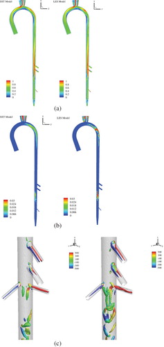
The vortical structures in the aorta are visualized using the second invariant of the rate-of-strain tensor (Q-criterion) and colored by helicity in Figure 7c. The resolution of the vortical structures improves and the vorticity magnitude predictions increase with the grid resolution, as expected. In addition, LES captures the details of the vortical structures better than URANS, in particular the hair-pin like structures. As shown in Figure 8, counter rotating vortex pairs and hair-pin vortices are predicted in the arteries, arch, near the renal artery branching, and at the iliac artery trifurcation.

Figure 8. Overall view of the vortical structures predicted in the feline aorta for healthy condition during decreasing systole. Results are shown using 11M grid. Inset figures show a zoomed in view of the vortical structure in the arch region, and the growth of the vortices near the renal and trifurcation regions.

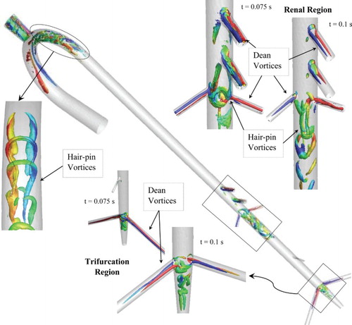
The counter-rotating vortices in the arteries and in the arch are identified to be Dean vortices, which have been well documented in the literature for internal flows with curvature such as curved pipes, the rabbit aortic arch, and for lung flows at bifurcations (Vincent, Plata, Hunt, Weinberg, & Sherwin, 2011). The Dean vortices are generated due to the imbalance in the centrifugal force and radial pressure gradient in the curved regions, i.e. either at arches or bifurcations/branching (Kalpakli, Örlü, Tillmark, & Alfredsson, 2011). In the arch, the counter-rotating limbs of the vortices cause lifting on each other, leading the vortices to move towards the outer wall and attach to form multiple hair-pin structures, consistent with the formation of hair-pin structures in near-wall turbulence (Zhou, Adrian, Balachandar, & Kendall, 1999).

The vortex in the renal branching region is attached to the posterior wall with counter-rotating vortex limbs protruding from the aorta-CrMA and/or aorta-celiac artery intersection. Richardson, Pivkin, Karniadakis, and Laidlaw (2006) identified that the counter-rotating vortices in the aorta are the secondary motions formed to balance the momentum loss via Dean vortices through artery branches. These counter-rotating vortices show lifting and merging similar to the hair-pin structures. The trifurcation region shows complicated vortical structures due to entanglement of Dean vortices in the left and right iliac arteries and secondary vortices in the common iliac artery.

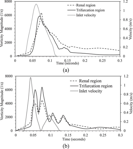
Figure 9a shows the growth and decay of the peak vorticity magnitude in the renal branching and trifurcation regions during the cardiac cycle. Both renal and trifurcation regions show similar vortex generation and decay trends. The vorticity generation starts close to the peak systole, and reaches a maximum during the decreasing systole due to the formation of hair-pin structures. The vorticity magnitude decays during diastole as the hair-pin vortices are stretched and advected downstream.

Figure 9. Growth and decay of the peak vorticity magnitude in feline renal artery and trifurcation regions over a cardiac cycle for (a) healthy and (b) HCM conditions obtained using 11M grid.

4.4. Predictions of feline aorta flow for HCM conditions (Cases 5 and 6)

As shown in Table 1, for HCM condition the mass flow through the arteries in the arch increases by 30%, shows less than 10% change in the abdominal arteries, and decreases by 50% in the iliac arteries, when compared with results from healthy condition. The artery outflows over the cardiac cycle show a bi-modal pattern, except for the iliac (Figure 6a). The flow rate peaks are coincident with the primary and secondary systole peaks. Abdominal arteries show backflow in between the primary and secondary systole peaks. The iliac artery shows a tri-modal flow pattern with the earliest peak at the peak primary systole, and backflows during the increasing secondary systole and in diastole (Figure 6b).

The flow during the increasing and peak primary systole is very similar to that of the healthy condition (refer to Bhushan et al., 2015). However, the flow acceleration in the abdominal aorta is significantly lower. The highest wall stress is predicted at the peak primary systole, with peak values mostly at the infra-renal aorta cross-section. The peak wall stresses are about 25% higher than those for healthy condition. The flow during the decreasing primary and increasing secondary systole shows several recirculation regions near the posterior wall of renal artery and at the iliac arteries, and they are more pronounced than those in the healthy condition. This phase shows the highest turbulence levels (TI ∼ 25%) and turbulence is spread over a wider area throughout the thoracic and abdominal aorta region.

Vortical structures in the aortic arch, renal, and trifurcation regions are similar to the healthy condition. As shown in Figure 9b, vorticity generation starts close to the peak primary systole, and shows two peaks, one during decreasing primary systole and a second during increasing secondary systole. The vortex strength is somewhat higher for the second peak, and the vorticity magnitudes in the trifurcation region are higher compared to those in the renal region. The peak vorticity magnitude in the trifurcation region is similar to the healthy condition, whereas the vortex is weaker in the renal region. The decay of the vortices is slower compared to the healthy condition due to the backflow from the arteries, which delays the advection of vortices.

4.5. Predictions of particle trajectory pattern (Cases 7 and 8)

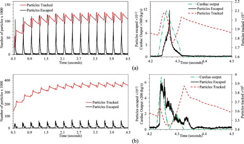
For the particle transport predictions, approximately 100 particles were uniformly distributed over the inlet at every time step during systole. Thus, for 15 cardiac cycle simulations, a total of 2.25M particles were injected into the aorta flow. In a clinical situation, the number of circulating free thrombi will be substantially smaller than what is simulated here. The large numbers of particles are modeled in order to account for a wide variety of possible thrombi paths through the aorta and their probabilistic impact locations on the aortic wall. Figure 10 shows the particle tracking time history over the 15 cardiac cycles for healthy and HCM conditions. For healthy condition, the number of remaining fluid-borne particles tracked converges by the 6th cycle to approximately 110 K, whereas for HCM convergence is obtained by the 9^th cycle to approximately 375 K particles. Beyond this point, the number of tracked particles exhibits a limit cycle behavior with insignificant cycle-to-cycle variation. Because the particles are randomly distributed at each time step, this result confirms that a sufficient number of particles are used in the simulations, since the use of too few particles would be expected to result in stochastic variations from one cycle to the next. Particle residence time history over a cardiac cycle shows that for the healthy condition the particles accumulate in the aorta mostly during increasing systole and the later part of the decreasing systole. For the HCM condition, the particles accumulate mostly during secondary systole.

Figure 10. Time history for particle deposition over 15 feline cardiac cycles (left panel), and particles injected, tracked and escaped during a cardiac cycle (right panel) for (a) healthy and (b) HCM conditions.

As summarized in Table 1, for the healthy condition about 4% of the injected particles are trapped in the aorta, whereas for the HCM condition about 15% of the particles are trapped. For both healthy and HCM conditions, around 40% of the injected particles did not terminate in wall impaction and were transported into the abdominal section. In the healthy condition, approximately 24% of the particles escape from the abdominal arteries and 10% from the trifurcation arteries. For the HCM condition, 21% of the particles escape from the abdominal arteries and 4% from trifurcation arteries. This suggests that particle accumulation in the HCM condition is primarily due to a decrease in the number of particles exiting the iliac arteries. This is consistent with the particle distribution shown in Figure 11, which shows that particles with the longest residence times reside in the thoracic and lower abdominal aorta.

Figure 11. Distribution of particles in feline aorta colored using residence time for (a) healthy and (b) HCM conditions. Only the particles with residence time more than 2 seconds or 6 cardiac cycles are shown (Left Panel). Mean (Middle Panel) and RMS (Right Panel) of axial velocity over a cardiac cycle.

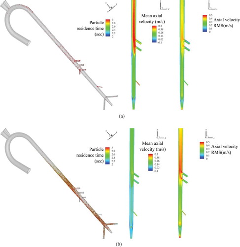
To quantify differences in the particle accumulation pattern between healthy and HCM conditions, the mean and RMS of axial velocity over an entire cardiac cycle is studied in Figure 11. The HCM condition predicts approximately 31% lower averaged axial flow and 28% higher RMS throughout the abdominal aorta compared to the healthy condition. Close to the trifurcation, averaged axial velocity is lowest and RMS is highest. An elevated RMS suggest that the HCM condition flow undergoes significant fluctuations compared to healthy condition, thus vortex advection is sluggish resulting in slower vortex decay causing entrapment of the particles.

5. Conclusions

Pulsatile flow simulations with particle transport have been presented in an idealized feline aorta geometry for healthy and HCM heart conditions to understand the role of aortic flow in entrapment of thrombi. To achieve the objectives CFD simulations are performed for healthy human aorta, healthy feline aorta, and HCM feline aorta flows; and the characteristics of the aortic flow dynamics and possible path line behavior of transported free thrombi are evaluated, and the role of aortic flow in entrapment of thrombi is discussed. The primary contributions of the study are: (a) development and validation of a novel iterative mass flow rate boundary condition for pulsatile flows, which is validated for healthy human abdominal aorta flow predictions; and (b) detailed investigation of fluid physics for aorta flow in HCM versus healthy heart conditions, including variation in flow rate and structures, vortex dynamics, and particle transport and residence times, as well as the potential impact on thrombogenesis.

The study demonstrated that for pulsatile flow Q_BC acts as a resistance-type boundary condition, but fails to accurately satisfy the outflow conditions. The proposed iterative I-Q_BC model addresses this issue, which is equivalent to in-simulation estimation of the outlet flow-resistance coefficient. The I-Q_BC predictions agree well with experimental data for healthy human abdominal aorta simulations, and are comparable to previously documented Womersley boundary condition predictions. However, both the I-Q_BC and Womersley boundary condition predictions show low amplitude secondary peak and trough in diastole, whereas experiments show almost uniform flow. For exploratory simulations for which the expected averaged flow rate from the arteries are not known, such as HCM condition, the target outlet mass flow rates in healthy conditions are used. Such an approach is justified because the flow-resistance from the downstream vasculature is expected to be approximately the same for the two conditions.

For the feline aorta case, a grid verification study shows that numerical uncertainties in the simulations using 4.2M to 11M grids are reasonably small, around 3.3%. The medium grid with 4.2M cells is found to be sufficient to resolve the overall flow structure; however, the finer grids are recommended for use with LES to allow better resolution of vortical structures. The flow primarily shows counter-rotating Dean vortices in the arch, artery branches, and in the abdominal aorta. The limbs of the Dean vortices cause lifting on each other, leading to the formation of hair-pin structures, primarily in the renal branching and trifurcation regions.

In the HCM condition, flow through abdominal arteries shows < 10% change, but iliac arteries show 50% lower flow, when compared to healthy conditions. HCM condition predictions also show significantly larger recirculation regions (and greater vortex strength) that persist longer compared to the healthy condition, causing the flow to be more sluggish. The overall sluggish flow and vortex decay results in entrapment of particles in the thoracic aorta and in the lower abdominal aorta before the trifurcation. The results are consistent with the observations of Kittleson et al. (1999), who reported that thrombi localize near the trifurcation for 71% of feline cases.

Finally, this study demonstrates that CFD can add insight to the relationship between ventricular pathophysiology and free thrombi transport in the aorta, potentially informing clinical decisions for improved treatment and management of saddle thrombus and other associated risks. One of the most notable differences between the simulations and the experiment is the diastole flow dynamics. The differences in the diastole flow are not expected to affect the flow separation or the vortex generation and decay predictions, as they occur primarily during systole. The predictions can be further improved by using a boundary layer profile for the inflow velocity. However, as the diastole predictions follow the inflow pulsatile behavior, it is not expected to address the differences. The differences could be potentially due to experimental uncertainties, therefore more detailed validation data are required. The artery bifurcations play a major role in the growth/decay of the vortical structures and affect the local flow and thrombus transport patterns. Simulations using patient-specific geometries may therefore be useful in drawing reliable conclusions. Future research efforts will focus on further improvement to the overall modeling methodology, including the use of real aorta geometries obtained from medical imaging procedures, as well as modeling the effects of arterial wall deformation through the use of fluid-structure interaction methods.

Disclosure Statement

No potential conflict of interest was reported by the authors.

Additional information

Funding

This research was funded by Mississippi NSF EPSCoR grant EPS-0903787. https://www.nsf.gov/awardsearch/showAward?AWD_ID=0903787

Notes

1. Only key references closely related to this study are discussed for the sake of brevity.

2. The (resolved) TKE in LES, as shown in Fig. 8(b), is obtained using the URANS velocity field as mean flow.

References

- Adedoyin, A. A., Walters, D. K., & Bhushan, S. (2015). Investigation of turbulence model and numerical scheme combinations for practical finite-volume large eddy simulations. Engineering Applications of Computational Fluid Mechanics, 9(1), 324–342. doi: 10.1080/19942060.2015.1028151
- Benim, A. C., Nahavandi, A., Assmann, A., Schubert, D., Feindt, P., & Suh, S. H. (2011). Simulation of blood flow in human aorta with emphasis on outlet boundary conditions. Applied Mathematical Modelling, 35, 3175–3188. doi: 10.1016/j.apm.2010.12.022
- Bhushan, S., Borse, M., Robinson, B., & Walters, D. K. (2015). Turbulent simulations of particle deposition in feline aorta flow for hypertrophic cardiomyopathy heart conditions. ASME/JSME/KSME 2015 Joint Fluids Engineering Conference, Paper No. AJKFluids2015-4688, pp. V001T04A003, 8 pages.
- Bhushan, S., Walters, D. K., & Burgreen, G. W. (2013). Transitional and turbulent flow simulations in FDA’s benchmark nozzle and capillary tube. Cardiovascular Engineering and Technology, 4(4), 408–426. doi: 10.1007/s13239-013-0155-5
- Cheema, T. A., Kim, G. M., Lee, C. Y., Hong, J. G., Kwak, M. K., & Park, C. W. (2014). Characteristics of blood vessel wall deformation with porous wall conditions in an aortic arch. Applied Rheology, 24, 24590, 1–8.
- Deep, D. (2013). A study of blood flow in normal and diseased aorta (MS thesis). Purdue University.
- Fedosov, D. A., Noguchi, H., & Gompper, G. (2014). Multiscale modeling of blood flow: From single cells to blood rheology. Biomechanics and Modeling in Mechanobiology, 13, 239–258. doi: 10.1007/s10237-013-0497-9
- Ferasin, L. (2009). Feline myocardial disease, diagnosis, prognosis and clinical management. Journal of Feline Medicine and Surgery, 11, 183–194. doi: 10.1016/j.jfms.2009.01.002
- FLUENT. (2006). User Guide FLUENT 6.3, FLUENT Inc. Centerra Resource Park, 10 Cavendish Court, Lebanon, NH 03766, USA.
- Gardhagen, R., Carlsson, F., & Karlsson, M. (2015). Large Eddy simulation of pulsating flow before and after CoA repair: CFD for intervention planning. Advances in Mechanical Engineering, 7(2), 971418. doi: 10.1155/2014/971418
- Howell, B. A., Kim, T., Cheer, A., Dwyer, H., Saloner, D., & Chuter, T. (2007). Computational fluid dynamics within bifurcated abdominal aortic stent-grafts. Journal of Endovascular Therapy, 14(2), 138–143. doi: 10.1177/152660280701400204
- Huo, Y., Guo, X., & Kassab, G. S. (2008). The flow field along the entire length of mouse aorta and primary branches. Annals of Biomedical Engineering, 36, 685–699. doi: 10.1007/s10439-008-9473-4
- Johnston, B. M., & Owen, D. A. (1977). Tissue blood flow and distribution of cardiac output in cats: Changes caused by intravenous infusions of histamine and histamine receptor agonists. British Journal of Pharmacology, 60, 173–180. doi: 10.1111/j.1476-5381.1977.tb07738.x
- Kalpakli, A., Örlü, R., Tillmark, N., & Alfredsson, P. H. (2011). Pulsatile turbulent flow through pipe bends at high Dean and Womersley numbers. Journal of Physics: Conference Series, 318(9), 092023, 1–10.
- Karmonik, C., Bismuth, J. X., Davies, M. G., & Lumsden, A. B. (2008). Computational hemodynamics in the human aorta: A computational fluid dynamics study of three cases with patient-specific geometries and inflow rates. Technol Health Care, 16(5), 343–354.
- Khanafer, K., & Berguer, R. (2009). Fluid-structure interaction analysis of turbulent pulsatile flow within a layered aortic wall as related to aortic dissection. Journal of Biomechanics, 42, 2642–2648. doi: 10.1016/j.jbiomech.2009.08.010
- Kittleson, M. D., Meurs, K. M., Munro, M. J., Kittleson, J. A., Liu, S. K., Pion, P. D., & Towbin, J. A. (1999). Familial hypertrophic cardiomyopathy in maine coon cats: An animal model of human disease. Circulation, 99, 3172–3180. doi: 10.1161/01.CIR.99.24.3172
- Lipowsky, H. H., Usami, S., & Chien, S. (1980). In viva measurements of “Apparent viscosity” and Microvessel Hematocrit in the mesentery of the cat. Microvascular Research, 19, 297–319. doi: 10.1016/0026-2862(80)90050-3
- Maron, B. J., Gottdiener, J. S., Arce, J., Rosing, D. R., Wesley, Y. E., & Epstein, S. E. (1985). Dynamic subaortic obstruction in hypertrophic cardiomyopathy: Analysis by pulsed Doppler echocardiography. Journal of the American College of Cardiology, 6, 1–15. doi: 10.1016/S0735-1097(85)80244-8
- Maron, B. J., & Maron, M. S. (2013). Hypertrophic cardiomyopathy. The Lancet, 381, 242–255. doi: 10.1016/S0140-6736(12)60397-3
- McGarry, M., Hitt, D. L., & Harris, T. R. (2008). Leakage rates from a punctured vessel under pulsatile flow conditions. Engineering Applications of Computational Fluid Mechanics, 2(3), 275–283. doi: 10.1080/19942060.2008.11015228
- Menter, F. R. (1994). Two-equation Eddy-viscosity turbulence models for engineering applications. AIAA Journal, 32(8), 1598–1605. doi: 10.2514/3.12149
- Moore, J. E., & Ku, D. N. (1994). Pulsatile velocity measurements in a model of the human abdominal aorta under resting conditions. Journal of Biomechanical Engineering, 116, 337–346. doi: 10.1115/1.2895740
- Moore, J. N., Ku, D. N., Zarins, C. K., & Glagov, S. (1992). Pulsatile flow visualization in the abdominal aorta under differing physiologic conditions: Implications for increased susceptibility to atherosclerosis. Journal of Biomechanical Engineering, 114, 391–397. doi: 10.1115/1.2891400
- Olufsen, M. S. (1999). Structured tree outflow condition for blood flow in larger systemic arteries. American Journal Physiology, 276, 257–268.
- Pasipoularides, A. (2011). Fluid dynamic aspects of ejection in hypertrophic cardiomyopathy. Hellenic Journal of Cardiology, 52, 416–426.
- Perktold, K., & Rappitsch, G. (1995). Computer simulation of local blood flow and vessel mechanics in a compliant carotid artery bifurcation model. Journal of Biomechanics, 28, 845–856. doi: 10.1016/0021-9290(95)95273-8
- Richardson, P. D., Pivkin, I. V., Karniadakis, G. E., & Laidlaw, D. H. (2006). Blood flow at arterial branches: Complexities to resolve for the angioplasty suite. In V. N. Alexandrov et al. (Eds.), ICCS 2006, Part III, LNCS 3993 (pp. 538–545). Reading, UK: Springer-Verlag Berlin Heidelberg.
- Robertson, E., Choudhury, V., Bhushan, S., & Walters, D. K. (2015). Verification and validation of OpenFOAM numerical methods and turbulence models for incompressible flows. Computers and Fluids, 123, 122–145. doi: 10.1016/j.compfluid.2015.09.010
- Samii, V. F., Biller, D. S., & Koblik, P. D. (1998). Normal cross-sectional anatomy of the feline thorax and abdomen: Comparison of computed tomography and cadaver anatomy. Veterinary Radiology Ultrasound, 39(6), 504–511. doi: 10.1111/j.1740-8261.1998.tb01640.x
- Sorensen, E. N., Burgreen, G. W., Wagner, W. R., & Antaki, J. F. (1999). Computational simulation of platelet deposition and activation: I. Model development and properties. Annals of Biomedical Engineering, 27, 436–448. doi: 10.1114/1.200
- Taylor, C. A., Hughes, T. J. R., & Zarins, C. K. (1999). Effect of exercise on hemodynamic conditions in the abdominal aorta. Journal of Vascular Surgery, 29, 1077–1089. doi: 10.1016/S0741-5214(99)70249-1
- Vincent, P. E., Plata, A. M., Hunt, A. A., Weinberg, P. D., & Sherwin, S. J. (2011). Blood flow in the rabbit aortic arch and descending thoracic aorta. Journal of The Royal Society Interface, 8, 1708–1719. doi: 10.1098/rsif.2011.0116
- Walters, D. K., Burgreen, G. W., Lavallee, D. M., Thompson, D. S., & Hester, R. L. (2011). Efficient, physiologically realistic lung airflow simulations. IEEE Transactions on Biomedical Engineering, 58, 3016–3019. doi: 10.1109/TBME.2011.2161868
- Walters, D. K., & Luke, W. H. (2011). Computational fluid dynamics simulations of particle deposition in large-scale, multi-generational lung models. ASME Journal of Biomechanical Engineering, 133, 011003, 1–8.
- Womersley, J. R. (1957). Oscillatory flow in arteries: The constrained elastic tube as a model of arterial flow and pulse transmission. Physics in Medicine and Biology, 2, 178–187. doi: 10.1088/0031-9155/2/2/305
- Zhou, J., Adrian, R. J., Balachandar, S., & Kendall, T. M. (1999). Mechanisms for generating coherent packets of hairpin vortices in channel flow. Journal of Fluid Mechanics, 387, 353–396. doi: 10.1017/S002211209900467X