Numerical investigations of the flow induced oscillation of a torque converter

Abstract

The flow induced oscillation of a three-element torque converter was investigated numerically under various operational conditions. A two-way coupling fluid–structure interaction simulation was performed using ANSYS-Fluent along with the ANSYS Transient Structural module. The fluid pressure excitation and the dynamic structure response were investigated at various turbine/pump rotation speed ratios . The maximum pressure blade load and structural deflections were observed in the stall condition, corresponding to the highest torque transmission ratio. The pressure pulsations and structure oscillations were monitored at locations selected on the basis of time-averaged distributions. The turbine oscillations were dominated by the frequency of pump blade passing at . The stator always oscillated under impact from the upstream flow with the dominating pump shaft frequency. Both the time-averaged and instantaneous features revealed that the pump oscillations were almost independent of SR.

Keywords:

• Flow induced oscillation
• fluid–structure interaction
• computational fluid dynamics
• torque converter

1. Introduction

A torque converter has been widely utilized as a major integral component of auto-transmissions for decades. The working fluid circulates in a closed loop to transfer and multiply the driving torque of the engine. The increased torque transmission ratio and reduced housing size for a higher power density result in stronger unsteady flow pressure excitation. High-amplitude fluid pressure pulsation acting on the blade rows causes structure oscillation and stress, which may lead to severe instability problems such as fatigue cracks (Wang, Quant, & Kolios, 2016).

The investigation of pressure excitations is essential for gaining insight into the structural response (Trivedi, Agnalt, & Dahlhaug, 2017; Trivedi & Cervantes, 2017). Multiple studies have investigated the flow behavior in three-element torque converters. Kraus, Flack, Habsieger, Gillies, and Dullenkopf (2005) studied the unsteady flow induced by the pump/turbine blades passing. It was observed that the turbine inlet flow is significantly periodic and the pump exit flow shows independence of the turbine blades passing, similar to the results obtained by Browarzik (1994). Brun and Flack (1997) measured the unsteady velocity field in the turbine through laser velocimetry at two typical speed ratios: 0.065 and 0.800. In their research, the speed ratio had a significant impact on the pressure pulsation in the stator. Dong, Lakshminarayana, and Maddock (1998) experimentally demonstrated that the pressure pulsation in the flow passages is dominated by two frequencies, respectively corresponding to the rotor shaft rotation and the flow interaction between the rotor and stator. In hydro-turbomachinery, such wake instability induced by the speed difference of a rotor and a stator or two rotors is one of the major sources of pressure pulsations, which further induce structure oscillations (Anup, Thapa, & Lee, 2014; Franke, Powell, Fisher, Seidel, & Koutnik, 2005; Rodriguez, Egusquiza, & Santos, 2007; Spence & Amaral-Teixeira, 2009).

Attention has been given to the application of numerical fluid–structure interaction (FSI) simulation to investigate the flow induced oscillations in various types of hydraulic turbomachine. For instance, Zhang, Guo, and Wang (2007) performed a transient FSI simulation to study the turbulent flow in a Francis turbine. They suggested that the blade oscillations were induced by the distorted wakes generated by the flow passing from the rotating turbine to the fixed guide vanes. Transient FSI simulations were also run on a single-blade pump by Pei, Dohmen, Yuan, and Benra (2012) and they observed that the normal structural stress caused by the fluid pressure was significantly higher than the tangential stress caused by flow-structure friction. Morris, O'Doherty, O'Doherty, and Mason-Jones (2016) performed static FSI simulations to investigate the blade deformation and the associated hydrodynamic performance variation of a tidal turbine.

As a consequence, although the unsteady flow fields in torque converters have been studied extensively, the flow induced oscillation problems are far from being understood. In our research, systematic two-way FSI simulations were performed to characterize both the pressure pulsations and structure oscillations. The specific setting for the numeral FSI simulation is described in Section 2; the results and a discussion are provided in Section 3; and main conclusions are summarized in Section 4.

2. Fluid–structure interaction simulation

In this study, FSI simulations were performed with the ANSYS 15.0 multi-field coupling solver system. Iterations were staggered between two solvers: a computational fluid dynamics (CFD) calculation and a structural analysis based on the finite element method (FEM) for each timestep were conducted to obtain the coupled simulation results. The fluid pressure excitation was calculated with ANSYS-Fluent 15.0, whereas the responses of the structure were obtained with the ANSYS Transient Structural module. A two-way coupled data transfer for the fluid pressure and structure deflection was employed at the fluid–structure interfaces (Campbell & Paterson, 2011).

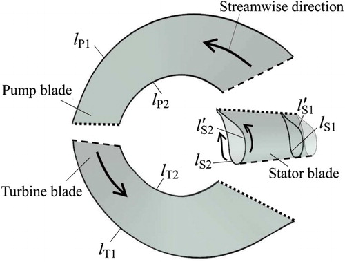
The torque converter model used in the current study consisted of three elements: a pump (P), a turbine (T), and a stator (S). A cross-sectional view of the torque converter is presented in Figure 1. The maximum working diameter and the width of the flow passage were and . The blades of the pump and turbine were made of steel of a constant thickness, while those of the aluminum stator had a typical hydrofoil cross-section. The blade mid-span angles of each component are presented in Figure 1(b) and Table 1. The cylindrical coordinate system of the torque converter was defined as follows: axial direction z, along the rotating shaft; tangential direction γ, in the torque converter rotational direction; and radial direction r, perpendicular to the shaft.

Figure 1. (a) Cross-section of torque converter; (b) blade angle system.

Table 1. Basic parameters of the torque converter model.

Component	Blade number	Inlet blade angle ()	Exit blade angle ()
Pump	= 41	−40	13
Turbine	= 37	48	−46
Stator	= 19	−26	61

2.1. CFD model

A model with whole-wheel flow passages was adopted to represent the entire fluid field in the torque converter. The five fluid domains in the pump (P), turbine (T), stator (S), housing chamber (H), and core chamber (C) were separated by the fluid–fluid interfaces. As shown in Figure 2(a), the interfaces comprised seven pairs of connected domain boundaries, following the flow direction, including the core chamber and pump inlet (C–P), pump exit and housing chamber (P–H), housing chamber and turbine inlet (H–T), turbine exit and core chamber (T–C), core chamber and stator inlet (C–S), stator exit and core chamber (S–C), and the interface between the two chambers (H–C). The working fluid circulated in a closed loop in the direction of the pump–turbine–stator movement. In the fluid domains, the FSI interfaces were defined as the inner passage surfaces of the blade, shell, and core. The unstructured tetrahedral meshes of the fluid domains were generated by the ANSYS ICEM, shown in Figure 2(b). A mesh independence analysis was performed to select the appropriate mesh density, presented in Figure 3. For torque converters, a calculated torque deviation less than 3 for each wheel component is considered to be independent of mesh density (Cheng Liu, Untaroiu, Wood, Yan, & Wei, 2015). Considering the calculation efficiency, a mesh size of 0.1 was adopted to generate the meshes of the fluid domains: the total mesh number was 3,892,138, where the pump was 916,585, the turbine 857,956, the stator 608,170, the core chamber 975,069, and the converter chamber 534,358.

Figure 2. (a) Schematic of fluid domains and boundary conditions; (b) meshes of fluid computational domains.

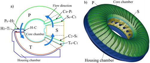
Figure 3. Mesh independence analysis.

In order to match the domain interfaces between the fluid and the structure during the calculation, the fluid mesh was allowed to deform to adapt to the deflected structure model. The mesh updating, enabled by the Spring smoothing method in ANSYS-Fluent 15.0, can prevent the occurrence of negative cell volumes (Degand & Farhat, 2002; Morris et al., 2016) to maintain the mesh quality.

The incompressible Navier–Stokes equations were solved using the SIMPLE algorithm, where the heat transfer wasn't taken into account (Chunbao Liu, Changsuo Liu, & Ma, 2015). The working fluid density was 830 kg·m⁻³, and the kinematic viscosity was 0.019 Pa·s. The k–ω shear-stress transport model (SST) was select as the turbulence model. Literature related to the CFD simulation in torque converters and similar turbomachines has validated the SST model's accuracy (Anup et al., 2014; Pei et al., 2012). The initial turbulence intensity was set to 1 and the simulation started from zero fluid velocity. Residual values of 10⁻⁴ for the flow continuity, velocity, and turbulent kinetic energy were adopted as the CFD solution convergence criterion.

2.2. Structural model

A whole-wheel structural model of the torque converter was established in the ANSYS Transient Structural module, as presented in Figure 4. The pump and turbine were made of constant thickness carbon steel while the cast stator was made of Al alloy. As part of the entire housing, the pump shell was 5.5 mm thick; the rest of the pump and turbine were 1.5 mm thick. Specific details of the material properties are presented in Table 2.

Figure 4. FSI interfaces on turbine, stator, and pump.

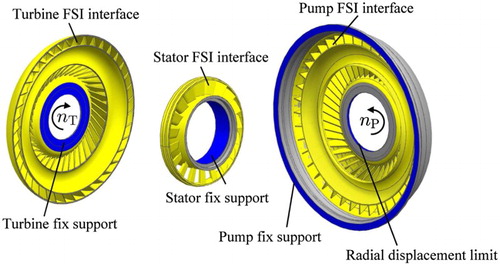
Table 2. Structure material properties.

Component	Material	E (GPa)	G (GPa)	ν	ρ (kg·m^−3)
Pump and turbine	Carbon steel (Ck45)	200	76.9	0.3	7850
Stator and Al alloy (UNS A03560)	71	26.7	0.33	2700

(Note: E is the Young's modulus; G is the shear modulus; ν is the Poisson's ratio; ρ is the material density).

In Figure 4, the coupling areas (displayed in yellow) and the boundary fixed supports (displayed in blue) were set corresponding to the FSI interfaces in the fluid domains. The turbine hub, the stator bypass clutch and the converter housing were treated as rigid structures. A radial displacement limit was set on the pump hub and a fixed support was set at the connection between the pump shell and the converter housing. For the structure FEM analysis, the unstructured meshes of the three wheels were generated by the ANSYS Mechanical Model, shown in Figure 5. The Solid186 shell element was selected for the simulation where the turbine has 147,798 elements, the stator 126,518 and the pump 288,623.

Figure 5. Meshes of turbine, stator, and pump for structure FEM analysis.

2.3. Methodology of FSI simulation

A two-way coupling method was applied in the FSI simulation. The co-simulation was established through the ANSYS Coupling System, where ANSYS-Fluent 15.0 and the ANSYS Transient Mechanical model were connected for the data exchange. The specific schematic for every timestep is presented in Figure 6. Several staggered coupling interactions were processed until the convergence criterion was reached. In the fluid solution, the fluid pressures obtained from the CFD calculations were transferred to the FSI interfaces of the structure model. The structural responses were presented as the boundary incremental displacement in the structure solution. The convergence criteria for data transfer was 0.01 – the same setting as adopted by Pei et al. (2012). At the end of each coupling interaction, the fluid mesh was updated to maintain its quality.

Figure 6. Flowchart of FSI simulation process.

The operating conditions of the torque converter were related to the speed ratio, , where and are the rotation speeds of the turbine and pump, respectively. The stall condition corresponds to SR=0.0. The value for was set at a constant 1500 rpm, and was increased from zero to 1200 rpm by increments of 150 rpm (), corresponding to the range . In order to capture the fluid regime and the structural responses as SR increased, the timesteps were selected based on the relation (1)

where is the speed difference between the pump and the turbine. The reference angle displacement was set to , which means the pump passed 1/5 of a turbine blade passage for every timestep interval. Various coupling timesteps are presented in Table 3. In total, 800 timesteps were adopted to capture the features of the fluid pressure pulsation and structure oscillation under various operating conditions.

Table 3. Timesteps for various operating conditions.

Speed ratio	0.0	0.1	0.2	0.3	0.4	0.5	0.6	0.7	0.8
)	2.0	2.2	2.4	2.8	3.3	3.9	4.9	6.5	9.8

3. Results and discussion

3.1. Performance tests of sample torque converter

Three performance characteristics obtained from both the experimental data and the FSI simulations are shown as functions of SR in Figure 7(a), including the torque transmission ratio TR, the efficiency of power transmission η and the pump capacity factor λ. TR is the quotient of the time-averaged torque of the turbine and the pump : . The efficiency η is defined as . The pump capacity factor represents the capability of the pump to absorb input power, given by the relation (2) where is the density of the working fluid in the torque converter, and is the acceleration due to gravity.

Figure 7. Performance comparison of sample torque converter obtained by experimental tests and FSI simulations.

As shown in Figure 7(b), the η obtained from the simulations are in good agreement with the experimental data, with a deviation of less than 5.0. Similar results can be found in Chunbao Liu et al. (2015). The good agreement of performance characteristics obtained from FSI simulation and experiments indicates that the fluid time-averaged pressure on the blade surface, which gives rise to , , and in the CFD part of the FSI simulations, is considered validated. The highest torque was observed at SR=0.0, indicating that the blades of each element had the highest pressure loading during the whole working SR range. In this paper, the stall condition (SR=0.0) is the primary case for investigating the characters of the pressure loading and structure response.

3.2. Time-averaged fluid pressure

The pressure distributions of all three elements at a speed ratio of zero are presented in Figure 8, where the contours were acquired at the final timestep. Concerning the turbine and stator, shown in Figures 8(a) and 8(b) respectively, the high flow pressure regions were observed around the leading edge of the blade pressure surface (PS) in the shell section. As for the stator blade suction surface (SS), the pressure loss covers almost the entire blade leading edge in the shell section, which suggests the occurrence of cavitation (Kowalski, Anderson, & Blough, 2005; Cheng Liu, Wei, Yan, & Weaver, 2016). Note that, in Figure 8(c), compared to the turbine and stator, the pump blades have a more uniform distribution in the radial direction; also, the pressure on the PS and SS are relatively lower. Three monitor points, , , and were set to record the pressure pulsations, which will be discussed later in this paper. The specific locations are listed in Table 4.

Figure 8. Pressure distribution in the stall condition, SR=0: (a) turbine, (b) stator, and (c) pump.

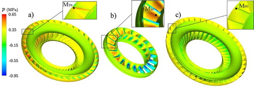
Table 4. Locations of monitoring points.

Monitoring points	Component	Specified location	Data recording
	Turbine	, = 0	p
	Turbine	, = 0
	Turbine	, = 1
	Turbine	round corner of shell, r/R = 0.52
	Stator	, = 0.2	p
	Stator	, = 0
	Stator	, = 0.4, PS
	Pump	, = 0	p
	Pump	, = 0
	Pump	edge of pump hub, r/R = 0.32

To reveal the characteristics of the flow pressure distributions on the blade surfaces further, several profiles were defined along the blade surface, as shown in Figure 9. The profiles in the shell and core blade sections were labeled , for the pump and , for the turbine. The stator blades had a typical airfoil shape, and each end of the profiles was set at the chord limitations along the z-direction. The profiles were labeled , on the pressure surfaces and , on the suction surfaces. The shell sections and were offset 0.2 towards the core chamber to cross through the high-pressure region, where is the maximum working diameter of the stator. The streamwise location ratio was defined as the streamwise position. The ranges from zero to one, which corresponds to the blade leading edge (dashed line) and trailing edge (dotted line).

Figure 9. Schematic of the streamwise blade profiles.

The blade pressure profiles in the shell and core sections for speed ratios of SR=0.0, 0.4 and 0.8 are presented in Figure 10. The solid curve represents the pressure distribution on the PS and the dashed curve is for the SS. The pressure coefficient is defined as (3) where p is the flow pressure on the blade surface, and is the pressure at = 0 of the pump blade shell section; is plotted as a function of the ratio , and the area enclosed by the two lines represents the blade pressure loading.

Figure 10. Profiles of time-averaged blade pressures for different SR values: (top to bottom) (a1)–(a3) turbine, (b1)–(b3) stator, and (c1)–(c3) pump.

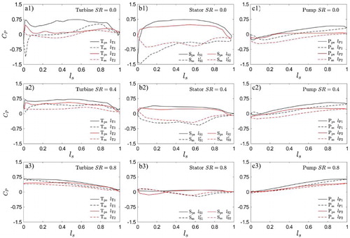
For the turbine at SR=0.0, shown in Figure 10(a1), the pressure distribution is extremely non-uniform along the streamwise direction. The highest blade loading is observed around the blade's leading edge in the shell section (), similar to the results obtained by By and Lakshminarayana (1995b). In Figure 10(b1), at the stator , the low pressure covers the region of the whole suction surface, where the highest blade loading of the stator is observed at . Similar stator pressure distributions were obtained by Dong, Korivi, Attibele, and Yuan (2002), Marathe, Lakshminarayana, and Maddock (1997) and Cheng Liu et al. (2016). By comparison, as shown in Figure 10(c1), the pressure distributions on both sides of the pump blade are more uniform, which lead to a much lower blade loading. In the shell section, the pressures on the PS and SS are reversed in the range as a result of the flow incidence effect induced by the sharp leading edge of the pump blade (By & Lakshminarayana, 1995a).

The pressure profiles at the higher speed ratios SR=0.4 and 0.8 are selected for presenting the variations of blade loading, other cases are not shown for brevity. The increasing SR causes a lower torque ratio TR corresponding to the reduction in blade loading. As illustrated in Figures 10(a2) and 10(a3), the pressures on the turbine blade surface becomes more uniformly distributed. The highest blade loading at SR=0.4 is observed at in the blade shell section, approximately the same position as SR=0.0. As to the stator, the blade loading variations at higher speed ratios are similar to the turbine's. At SR=0.8, shown in Figure 10(b3), a pressure reversal is found around the leading edge of the blade suction surface ( ∈ [0.0 0.3]). In Figures 10(c2) and 10(c3), increasing the SR induces a small-amplitude reduction in pump blade loading.

The pressure distributions in all cases reveal that, for the turbine and stator blades, regions close to the leading edge in the shell section has the highest difference in the stall condition SR=0.0. Increasing the SR significantly reduced the blade loading. The pump has a uniform pressure distribution and low-amplitude blade loading which is almost independent of the SR.

3.3. Deflections and stress distributions

The contours of the deflections of the pump, turbine, and stator at SR=0.0, acquired at the final timestep, are presented in Figure 11. For the turbine, shown in Figure 11(a), the maximum deflection occurs at the junction between the shell and blade leading edge, corresponding to the location of the maximum blade loading; whereas the structure deflection is assumed to be negligible in the area connected to the rigid turbine hub , where R=0.5D. A similar distribution is found for the stator, shown in Figure 11(b). In Figure 11(c), the maximum deflection of the pump occurs around the hub (), which is free to move along the axis direction. Generally for the turbine and stator, the total deflection diminishes with decreasing r along the radial direction.

Figure 11. Deflection distribution in the stall condition, SR=0: (a) turbine, (b) stator, and (c) pump.

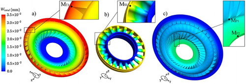
To provide a specific indication of the structure deflection (W) and von Miss stress () under various speed ratios, seven monitoring points were set in the high deflection and stress areas. , , , and are shown in the subplots of Figure 11. The positions of the monitor points are given in Table 4. To analyse the total deflection and its components in three directions, tangential , radial , and axial , the time-averaged blade deflections of the monitors on each element are presented in Figure 12.

Figure 12. Time-averaged deflections at various SR, obtained at blade monitoring points: (a) turbine , (b) stator , and (c) pump , .

For the turbine's leading edge in Figure 12(a), increasing SR leads to a gradually decreasing . The total deflection in the SR range is mainly constituted by the tangential deflection and axial deflection , while the radial deflection remains at a low amplitude level. At SR=0.4, as the results of lower pressure loading and the increasing centrifugal force of the turbine, the change its direction from negative to positive. At SR=0.8, and are the primary components of , and is close to W/D = 0. The deflection of the stator's leading edge has primary components similar to those of the turbine, shown in Figure 12(b). As discussed previously, compared to the turbine and stator, the pump blade has a much lower pressure loading, which leads to an almost constant low-amplitude deflection at the pump inlet , as shown in Figure 12(c). At the edge of the pump hub , owing to the structure connection limits, only two degrees of freedom exist: rotation around the z-axis and displacement in the z-axis direction (). As shown in Figure 12(c), increases slightly with larger SR.

The contours of the von Mises stress , as shown in Figure 13, acquired at the final timestep, present the stress distributions of each element at SR=0.0. In Figure 13(a), the stress concentrations of the turbine are observed in two areas, the trailing edge in the blade shell section and the round corner of the shell between the turbine hub and the blade cascade. For the stator, in Figure 13(b), owing to the large amplitude deflection of the stator core and the fixed constraint on the stator hub, the high stress is concentrated mainly in the blade shell section. The stress distribution of the pump is more uniform than those of the turbine and stator. In Figure 13(c), the stress concentration is observed at the leading edge in the pump blade shell section.

Figure 13. Von Mises stress distributions in the stall condition, SR=0: (a) turbine, (b) stator, and (c) pump.

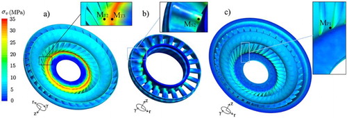
Corresponding to the stress concentration areas discussed above, the specific locations of several monitoring points are presented in Figure 13 subplots. As can be observed in Figure 14, for , on the turbine and on the stator, the high stress concentration occurs at SR=0.0. As the SR increases in the range , the for the turbine falls rapidly, while and have approximately the same at SR=0.6. Increasing the SR leads to a gradually decreasing on the stator . In contrast with the turbine and the stator, the maximum difference of is 2.04 over the whole range of SR, which is almost independent of SR.

Figure 14. Time-averaged stress at various SR values, obtained at the blade monitoring points.

3.4. Flow induced oscillation

To get insight into the inner relationship between unsteady fluctuating pressure excitation and the dynamic structure oscillation response, the spectral characteristics for the three elements were obtained via a Fast Fourier Transform (FFT) analysis. The operation conditions SR=0.0, 0.4 and 0.8 were selected to illustrate the spectral variations under the impact of increasing the SR. The spectra of other cases are not shown for brevity.

The spectra of both the fluid pressure pulsations and structure oscillations for the selected monitors at are shown in Figure 15. Figure 15(a1) shows two distinct frequency peaks: and ; here, is the frequency with which the pump blade passes relative to the turbine. Meanwhile, , where is the pump shaft frequency, and = /60. The highest speed difference between the pump and turbine at SR = 0.0 results in being the dominant frequency in the turbine. The pressure pulsations in the stator have the same frequencies under the impact from upstream, shown in Figure 15(a2); however, the becomes dominant owing to the reduced energy of the secondary frequency . The same frequency at was respectively observed by Marathe et al. (1997) in the turbine flow passages and by Y. F. Liu, Lakshminarayana, and Burningham (2001) on the stator blade surface. In Figures 15(b1) and 15(b2), , and their harmonic frequencies are also observed in the oscillation spectra as responses to the pressure excitation. Similar spectral phenomena were observed by Conrad, Weber, and Jung (2017), Huang, Oram, and Sick (2014) and Rodriguez et al. (2007) for hydraulic turbines. It is important to note that the pressure excitation frequency fades rapidly with increasing SR () before matching one of the eigenfrequencies of the turbine to cause the resonance phenomenon.

Figure 15. Spectra of the fluid pressure pulsations and structure oscillations at SR=0.0. (a1)–(a3) pressure pulsations; (b1)–(b3) structure oscillations.

Figure 15(a3) shows that the fluctuating pressure at the pump blade leading edge is dominated by the passing frequency of the stator relative to the pump: , with the same frequencies as those observed by Dong and Lakshminarayana (2001) in the pump flow field. Owing to the low-amplitude blade load discussed previously, no such frequency at is observed in the structural response.

As the turbine rotation speed increases, a dominant frequency transition occurs in both the pressure and oscillation spectra. At the higher speed ratio SR=0.4, shown in Figure 16(a1), the turbine passing frequency relative to the pump, , has the highest spectral energy, where . However, in Figure 16(b1), the turbine shaft frequency dominates the oscillation spectrum, with no clear spectral peak corresponding to , which indicates that the primary excitation force for the rotating turbine is the centrifugal force. In Figures 16(a2) and 16(b2), for the stator, the existence of reflects that the influence from upstream is still significant.

At the speed ratio SR=0.8, the torque ratio TR almost reaching 1.0, as discussed above, the blade loading is much lower than that at SR=0.0. As presented in Figures 17(a1) and 17(a3), is the dominant frequency at in the turbine and in the pump. In Figure 17(a2), multiple frequencies can be observed at the stator's leading edge , including and its harmonics, and , where is the turbine passing frequency relative to the stator, = . Marathe et al. (1997) obtained similar results and suggested that, owing to the closed-loop flow path of the torque converter, the unsteady frequencies induced by the interaction of the rotors and stators were superimposed, resulting in the observed combinations of blade passing frequencies.

Figure 16. Spectra of the fluid pressure pulsations and structure oscillations at SR=0.4. (a1)–(a3) pressure pulsations; (b1)–(b3) structure oscillations.

Figure 17. Spectra of the fluid pressure pulsations and structure oscillations at SR=0.8. (a1)–(a3) pressure pulsations; (b1)–(b3) structure oscillations.

4. Conclusions

The structure oscillations induced by the unsteady flow pressure pulsations in a torque converter were investigated through a two-way coupling, fluid–structure interaction simulation. The calculations and the data transmissions were performed under the co-simulation of the ANSYS-Fluent and the ANSYS Transient Structural module. The flow field and structural deflections were explored across a wide range of turbine/pump rotation speed ratios , with the result that the performance data including the torque transmission ratio TR and efficiency η match well the with the experimental results. The time-averaged results were investigated first to illustrate the distributions of the pressure and deflection under various SR values. The maximum deflections of the turbine and stator were found around the leading edge in the shell section, while the pump maximum deflection occurred at the edge of the pump hub owing to the structural limit. Increasing SR induced a lower TR and blade load, which further resulted in a reduction of structure deflection.

The unsteady fluid pressure excitation and the dynamic structure responses were monitored at selected locations based on the time-averaged distributions. At SR=0.0, the dominant frequency of the turbine oscillation was the same as the blade passing frequency of the pressure pulsation. Higher SR values () caused a spectral transition of the dominant pressure pulsation frequency from to the turbine blade passing frequency , while the oscillations were dominated by the turbine shaft rotation frequency , owing to which the pressure excitation was moderated. The oscillation frequencies of the stator always locked on the distinct frequency peaks in the pressure spectra with the dominating frequency at . The time-averaged and spectral features revealed that the pump oscillations were almost independent of the pressure variations caused by the changing speed ratio. With the application of FSI simulation, more understanding was gained regarding the inner relationship between pressure pulsation and structural response, which will benefit the prediction accuracy of the fatigue life and the lightweight design of torque converters.

Disclosure statement

No potential conflict of interest was reported by the authors.

Additional information

Funding

This work has been funded by the National Natural Science Foundation of China (NSFC) under Grant No. 51475041.

References

- Anup, K. C., Thapa, B., & Lee, Y. H. (2014). Transient numerical analysis of rotor–stator interaction in a Francis turbine. Renewable Energy, 65(8), 227–235.
- Browarzik V. (1994, June). Experimental investigation of rotor/rotor interaction in a hydrodynamic torque converter using hot-film anemometry. Proceedings of the 39th international gas turbine and aeroengine congress and exposition, The Hague, The Netherlands (pp. 13–16).
- Brun, K., & Flack, R. D. (1997). Laser velocimeter measurements in the turbine of an automotive torque converter: Part II – Unsteady measurements. Journal of Turbomachinery, 119(3), 655–662. doi: 10.1115/1.2841171
- By, R. R., & Lakshminarayana, B. (1995a). Measurement and analysis of static pressure field in a torque converter pump. Journal of Fluids Engineering, 117(1), 109–115. doi: 10.1115/1.2816798
- By, R. R., & Lakshminarayana, B. (1995b). Measurement and analysis of static pressure field in a torque converter turbine. Journal of Fluids Engineering, 117(3), 473–478. doi: 10.1115/1.2817286
- Campbell, R. L., & Paterson, E. G. (2011). Fluid–structure interaction analysis of flexible turbomachinery. Journal of Fluids and Structures, 27, 1376–1391. doi: 10.1016/j.jfluidstructs.2011.08.010
- Conrad P., Weber W., & Jung, A. (2017). Deep part load flow analysis in a Francis model turbine by means of two-phase unsteady flow simulations. Journal of Physics: Conference Series, 813, 1, Paper No. 012027. doi: 10.1088/1742-6596/813/1/012027.
- Degand, C., & Farhat, C. (2002). A three-dimensional torsional spring analogy method for unstructured dynamic meshes. Computers & Structures, 80, 305–316. doi: 10.1016/S0045-7949(02)00002-0
- Dong, Y., Korivi, V., Attibele, P., & Yuan, Y. (2002). Torque converter CFD engineering: Part I – Torque ratio and K factor improvement through stator modifications. SAE Technical Paper. Society of Automotive Engineers. doi: 10.4271/2002-01-0883.
- Dong, Y., & Lakshminarayana, B. (2001). Rotating probe measurements of the pump passage flow field in an automotive torque converter. Journal of Fluids Engineering, 123(1), 81–91. doi: 10.1115/1.1341202
- Dong, Y., Lakshminarayana, B., & Maddock, D. (1998). Steady and unsteady flow field at pump and turbine exits of a torque converter. Journal of Fluids Engineering, 120(3), 538–548. doi: 10.1115/1.2820696
- Franke, G., Powell, C., Fisher, R., Seidel, U., & Koutnik, J. (2005). On pressure mode shapes arising from rotor/stator interactions. Sound and Vibration, 39, 14–18.
- Huang, X., Oram, C., & Sick, M. (2014). Static and dynamic stress analyses of the prototype high head Francis runner based on site measurement. IOP Conference Series: Earth and Environmental Science, 22(3), Paper Number 032052. doi:doi: 10.1088/1755-1315/22/3/032052.
- Kowalski D., Anderson, C., & Blough, J. (2005). Cavitation detection in automotive torque converters using nearfield acoustical measurements (SAE Technical Paper 2005-01-2516). Society of Automotive Engineers. doi: 10.4271/2005-01-2516.
- Kraus, S. O., Flack, R., Habsieger, A., Gillies, G. T., & Dullenkopf, K. (2005). Periodic velocity measurements in a wide and large radius ratio automotive torque converter at the pump/turbine interface. Journal of Fluids Engineering, 127(2), 308–316. doi: 10.1115/1.1891150
- Liu, Y. F., Lakshminarayana, B., & Burningham, J. (2001). Flow field in the turbine rotor passage in an automotive torque converter based on the high frequency response rotating five-hole probe measurement: Part I – Flow field at the design condition (speed ratio 0.6). International Journal of Rotating Machinery, 7(4), 253–269. doi: 10.1155/S1023621X01000227
- Liu, C., Liu, C., & Ma, W. (2015). RANS, detached eddy simulation and large eddy simulation of internal torque converters flows: A comparative study. Engineering Applications of Computational Fluid Mechanics, 9(1), 114–125. doi:doi: 10.1080/19942060.2015.1004814.
- Liu, C., Untaroiu, A., Wood, H. G., Yan, Q., & Wei, W. (2015). Parametric analysis and optimization of inlet deflection angle in torque converters. Journal of Fluids Engineering, 137(3), 03411. doi:doi: 10.1115/1.4028596.
- Liu, C., Wei, W., Yan, Q., & Weaver, B. K. (2017). Torque converter capacity improvement through cavitation control by design. Journal of Fluids Engineering, 139(4), 041103:1–8. doi:doi: 10.1115/1.4035299.
- Marathe, B. V., Lakshminarayana, B., & Maddock, D. G. (1997). Experimental investigation of steady and unsteady flow field downstream of an automotive torque converter turbine and inside the stator: Part II – Unsteady pressure on the stator blade surface. Journal of Turbomachinery, 119(3), 624–633. doi: 10.1115/1.2841168
- Morris, C. E., O'Doherty, D. M., O'Doherty, T., & Mason-Jones, A. (2016). Kinetic energy extraction of a tidal stream turbine and its sensitivity to structural stiffness attenuation. Renewable Energy, 88, 30–39. doi: 10.1016/j.renene.2015.10.037
- Pei, J., Dohmen, H. J., Yuan, S. Q., & Benra, F. K. (2012). Investigation of unsteady flow-induced impeller oscillations of a single-blade pump under off-design conditions. Journal of Fluids and Structures, 35, 89–104. doi: 10.1016/j.jfluidstructs.2012.08.005
- Rodriguez, C. G., Egusquiza, E., & Santos, I. F. (2007). Frequencies in the vibration induced by the rotor stator interaction in a centrifugal pump turbine. Journal of Fluids Engineering, 129(11), 1428–1435. doi:doi: 10.1115/1.2786489.
- Spence, R., & Amaral-Teixeira, J. (2009). A CFD parametric study of geometrical variations on the pressure pulsations and performance characteristics of a centrifugal pump. Computers & Fluids, 38(6), 1243–1257. doi: 10.1016/j.compfluid.2008.11.013
- Trivedi, C., Agnalt, E., & Dahlhaug, O. G. (2017). Investigations of unsteady pressure loading in a Francis turbine during variable-speed operation. Renewable Energy, 133, 397–410. doi: 10.1016/j.renene.2017.06.005
- Trivedi, C., & Cervantes, M. J. (2017). Fluid–structure interactions in Francis turbines: A perspective review. Renewable and Sustainable Energy Reviews, 68, 87–101. doi: 10.1016/j.rser.2016.09.121
- Wang, L., Quant, R., & Kolios, A. (2016). Fluid structure interaction modelling of horizontal-axis wind turbine blades based on CFD and FEA. Journal of Wind Engineering and Industrial Aerodynamics, 158, 11–25. doi: 10.1016/j.jweia.2016.09.006
- Zhang, L., Guo, Y., & Wang, W. (2007). Large eddy simulation of turbulent flow in a true 3D Francis hydro turbine passage with dynamical fluid–structure interaction. International Journal for Numerical Methods in Fluids, 54(5), 517–541. doi: 10.1002/fld.1408