Aerodynamic effects of the gap spacing between adjacent vehicles on wind tunnel train models

Abstract

A certain gap spacing between adjacent vehicles is usually inevitable in wind tunnel force tests of high-speed trains under no crosswind, which may affect the wind tunnel test results. Thus, to understand the influence of gap spacings on the train aerodynamics, the aerodynamic drag, pressure distributions and airflow structures of 1/8th-scale high-speed train models with gap spacings of 0, 5, 8, 10, 20, and 30 mm were studied using RANS based on SST k-ω turbulence model. The simulation method was verified by the wind tunnel experiment data. The results show that the gap spacing significantly affects the airflow structure around inter-car gap and aerodynamic resistances of train models. For the high-speed train model scaled at 1/8th at zero yaw, compared with gap spacing of 0 mm, the gap spacings lead to a significant reduction in the aerodynamic drag of the head car and an increase in that of the tail car, whereas which of the middle car is not significant. The maximum difference of the drag coefficient of the entire train model is smaller than 2.0%. When the gap spacing does not exceed 8 mm, the discrepancies of the drag coefficients of three cars are within 6.15%.

KEYWORDS:

• High-speed train
• aerodynamic drag
• gap spacing
• RANS
• pressure distribution
• boundary layer

1. Introduction

For the train operating in the open air with no crosswind, the aerodynamic resistance is almost proportional to the square of train speed (Brockie & Baker, 1990). Thus, for the HSTs (high-speed trains) with a higher speed, the proportion of the aerodynamic drag becomes larger. A HST (high-speed train) desired is usually expected to have the characteristic of high efficiency and low energy consumption (Baker, 2014a; Raghunathan et al., 2002; Raina et al., 2017; Zhang, Wang, et al., 2018), which is closely related to the aerodynamic drag. Thus, A comprehensive understanding of the aerodynamic drag and other performances of the HST cruising at zero yaw is essential for the design and operation of HSTs. Currently, the wind tunnel tests have already become one of the most widely used experiment methods to investigate the aerodynamic drag of HSTs (Baker, 2014b; Bocciolone et al., 2008; Niu et al., 2016; Niu, Zhou, Liang, et al., 2018; Xiang et al., 2017; Zhang, Yang, et al., 2018), due to the advantages of the measurement accuracy and controlled environment conditions. Hence, the aerodynamic drag and other performances of the HSTs cruising at zero yaw angle have been widely investigated based on the wind tunnel tests (Brockie & Baker, 1990; Kwon et al., 2001; Willemsen, 1997; Zhang, Yang, et al., 2018).

As known to all, wind tunnel tests are based on the similarity principle and the actual full-scale flow field is reproduced by the reduced-scale flow field in the wind tunnel. However, the complete similarity between the flow fields around the HST model and prototype is usually difficult to achieve, due to the model and ground configuration simplification and other reasons, thus, the deviation between the models and prototypes should been treated carefully, avoiding unrealistic and artificial airflows (Munson et al., 2009). The similarity problems in the train wind tunnel tests have been widely investigated (Sicot et al., 2018). Sicot et al. (2018) performed an experiment in a wind tunnel to research the effect of the scale of reproduction of the geometric details on train models during the wind tunnel test, and the result showed that the existence of these geometric artifacts significantly affects the forces and moments measured in the wind tunnel tests. Schober et al. (2010) investigated the effects of three different ground configurations on the aerodynamic forces and tuft flow visualization measured in the wind tunnel tests, which demonstrated that different ground configurations had significant influences on the measured aerodynamic drag and airflow structure in the wind tunnel tests. J. Zhang et al. (2016) investigated the influence of the ground and wheel conditions on the HST performances based on CFD, which indicated that different ground conditions changed the aerodynamic drag acting on the HST model and the airflow structure surrounding it. Thus, it can be seen that any small difference between the HST models and prototypes may affect the airflow structures around HST models, which may result in the variations of the aerodynamic drag performances of the HST.

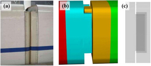
In the wind tunnel experiment, for accurate measurement of the aerodynamic loads of individual vehicle, it is general to fix vehicles on the floor plate separately with a certain gap spacing between adjacent vehicles, avoiding interactions between adjacent vehicles. Zhang, Wang, et al. (2018) specified that a gap between individual vehicles was necessary for wind tunnel tests, but did not elaborate on what the distance should be or give any recommendation about the appropriate spacing value. Zhang et al. (2016) underlined that to get precise and separate measurements of aerodynamic forces of individual vehicles, there should be a gap of 8 mm between adjacent vehicles in 1/8th scale with the nest form structure shown as Figure 1(b), but the effect of the gap on the results was not given. Zhang, Yang, et al. (2018) indicated that the nested form shown in Figure 1(b) could be applied in the wind tunnel test, to avoid the undesired contact and collision and achieve the geometric similarity between the HST scale model and prototype shown as Figure 1(a) (CRH in China), whereas the effect of gap spacings was not given out. However, in actual, adjacent vehicles for HSTs are usually connected by internal and external windshields, giving a gap spacing of zero, thus, this deviation between train models and prototypes may lead to certain discrepancies of the aerodynamic results. Moreover, for the scale train model, different aerodynamic performances may result due to the differences in the gap spacing. Thus, Li et al. (2019) investigated 10 different gap spacings (shown in Figure 1(c)) on the aerodynamic drag of the 1/8th scale HST model and showed that the gap spacing should be smaller than 10 mm. However, the different gap spacings studied were achieved by moving the spatial position of certain vehicles longitudinally, and this movement resulted in not only the variation of the gap spacing, but that of the relative position between model train vehicles and the distance between the nose tips of the head and tail cars, i.e. the variation of the total length of the scale HST model between different studied cases. This may have undesired additional effects on the evolution of the airflow structures surrounding the HST model, which may eventually have an effect on the result, except for that only caused by variations of gap spacings. Thus, it is necessary and conservative to investigate the influence of gap spacings on the airflow structures and train aerodynamic resistance, while avoiding discrepancies of the total length and relative positions of vehicles between different studied cases, which gives impetus to study the gap spacing effect avoiding the variation of other parameters.

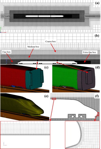
Figure 1. Geometric structures of inter-car gap regions: (a) Prototype HSTs in China; (b) Wind tunnel 1/8th-scale HST model (Zhang, Yang, et al., 2018); (c) Numerical train model used by Li et al. (2019).

Hence, in this study, the variations of gap spacings are obtained by installing the internal and external windshields with different thicknesses on the end walls of vehicles, and the spatial position of vehicles and other structures are remained the same in different cases, and the nests form structure shown in Figure 1(b) was adopted, for the wide application. The aerodynamic drag and pressure distribution of the train model with different gap spacings at zero yaw angle were studies based on CFD, which has been widely used in the study of the train aerodynamics and other fields (Akbarian et al., 2018; Ghalandari et al., 2019; Mou et al., 2017; Niu et al., 2020). The structure of this study is as follows: the numerical details were introduced in Section 2. In Section 3, the validations of algorithm reliability and grid convergence were conducted. The result analyses and final conclusions were given in Sections 4 and 5, respectively.

2. Numerical analysis

2.1. Numerical method

Currently, the RANS, DES (detached eddy simulation), and LES (large-eddy simulations) are the main methods used for the study of train aerodynamics. Compared with the LES and DES, RANS can better balance the numerical predication accuracy and computational cost (He et al., 2019; Morden et al., 2015; Munoz-Paniagua et al., 2017), and has been successfully applied in the studies of the aerodynamic performances of HSTs and cars (Gao et al., 2019; Kurec, Remer, Mayer, et al., 2019; Liu et al., 2019; Xia et al., 2016). Meanwhile, considering that the main concerns of this study is the time-averaged properties of the aerodynamic quantities and surrounding flow field of the train model, thus the RANS was selected in this study. However, some details of the flow contained in the instantaneous fluctuations were discarded due to the time-averaging operations on the momentum equations (Versteeg & Malalasekera, 2007), thus, the SST k-ω model has been applied to model Reynolds stresses terms in the time-averaged momentum equations to predict the effects of the turbulence. The SST k-ω turbulence model was employed because it (Menter, 1994; Menter et al., 2003) was widely used because of its good prediction abilities for various turbulences and more precise simulations for adverse pressure–gradient boundary layer airflows and separations (ANSYS Inc, 2017; Li et al., 2018; Rahman et al., 2018; Raina et al., 2017).

In this study, the numerical simulations were performed in ANSYS Fluent based on the finite volume method. The pressure-velocity coupling was realized by the semi-implicit method for pressure-linked equations consistent algorithm implemented in the pressure-based solver. The Least Squares Cell Based was chosen for the discretization of gradients. And the second-order upwind scheme was adopted for the discretization of the momentum and k-ω equations. The convergence standard for the continuity equation is that the residual no more than 10e-5.

2.2. Computational train models and cases

The simplified 1/8th scale train model with a subgrade track used in this study was illustrated in Figure 2, which was built referring to the wind tunnel train models (Zhang, Yang, et al., 2018). According to the calculation formula of Reynolds number given in section 2.3, the HST model scaled at 1:8 gives a Reynolds number of $1.9\times 10^6$, under the uniform inflow flow velocity of 60 m/s herein. On the basis of the research results from other reports (Bell et al., 2014; Niu et al., 2016; Zhang, Yang, et al., 2018), it can be concluded that under the Reynolds number in this study, the Reynolds number have entered the self-simulation zone, and the Reynolds number has no significant influence on the flow field structures, thus, the Reynolds number effect on the train aerodynamic forces and pressure coefficient distribution is also very small and even negligible for this study, which means this 1/8th scale HST model is applicable herein. Furthermore, this 1/8th scale three-car HST model has been widely utilized for the research of the aerodynamic drag and other performances of HSTs without crosswind (Gao et al., 2019; Li et al., 2019; Niu, Wang, Zhang, et al., 2018; Zhang et al., 2016; Zhang, Wang, et al., 2018). The HST model consists of the head (6.88H), middle (6.6H) and tail (6.88H) cars, where H is the characteristic length scale, with the value of 0.4625 m in 1/8th scale and 3.7 m for a full-scale train. The simplified track and subgrade were built referring to the ground configuration for numerical simulations outlined in the CEN European Standard 14067-4 (2010), and the detailed dimensions were depicted in Figure 2(d). As shown in Figure 2(e), each vehicle body was divided into a near-gap part and a far-gap part (including the bogies), and there are two main purposes of dividing the body into two parts: one is to facilitate the grid refinement of the inter-car gap regions, thus obtaining the high quality grid and ensuring an appropriate number of grids; the other is to realize a clear analysis of the impact of gap spacings on different parts of train bodies. The near-gap parts for the head and tail cars are defined as tc2 and wc2, and the far-gap parts are defined as tc1 and wc1, respectively. Similarly, zc1 represents the far-gap part of the middle car, and the near-gap parts include zc2 and zc3.

Figure 2. Scaled train model: (a) 1:8th scale train used in the wind tunnel tests (taken from Zhang, Yang, et al. (2018)); (b) Perspective view of the model; (c) Schematic of the gap spacing studied in this paper; (d) Front view and (e) side view of the model employed in this study.

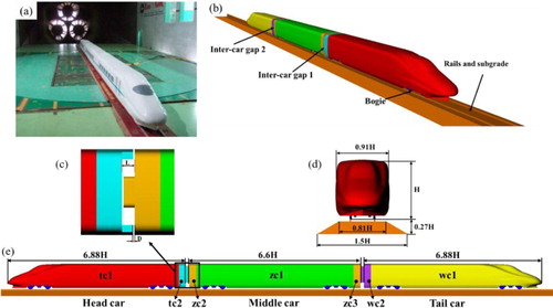
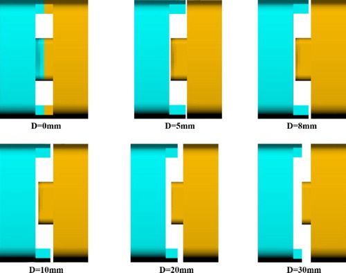
In the inter-car gaps 1 and 2, the internal windshields are attached to the walls at both ends of the middle car, whereas the external windshield structures are attached to the end walls of the head and tail cars. The gap spacing D depicted in Figure 2(c) represents the spacing between adjacent vehicles, with the same value in the two inter-car gaps in one studied case. And L was kept the same between different cases, which was 0.5 m for full-scale train and 0.0625 m in 1:8 scale, representing the distances between the end wall surfaces of adjacent vehicles. As shown in Figure 3, six different D values (0, 5, 8, 10, 20, and 30 mm) were studied here, and D = 0 mm, reflecting the real train, was studied for comparison with the other five gap spacings.

Figure 3. Different gap spacings in different train models.

2.3. Computational domain and boundary conditions

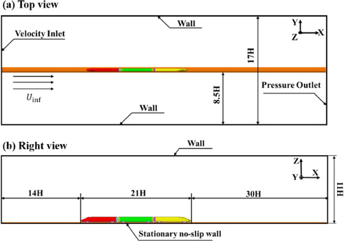
As illustrated in Figure 4, the main dimensions of the computational domain herein were depicted detailly, which was built according to the wind tunnel test (Zhang, Yang, et al., 2018) and CFD-based researches (Gao et al., 2019; Zhang et al., 2016). Whereas the length of the domain is slightly longer than that of the wind tunnel experiment section, and the distance between the tail car nose and the downstream boundary is more than twice that between the upstream boundary and the head car nose, ensuring a full development of the wake. The cross-section area of the HST model is 11.2${\text{m}}^2$ for a full-scale train and 0.175${\text{m}}^2$ in 1:8 scale, giving a blockage ratio of 0.438%. The uniform wind velocity of 60 m/s was assigned to the velocity inlet boundary, giving a Reynolds number of $Re=1.9\times {10}^6$ based on characteristic length H ($Re=\rho U_{inf}H/\mu$, where $\rho$ is the air density of 1.225 $\text{kg}/{\text{m}}^3$, $U_{\text{inf}}$ is the uniform incoming flow velocity, and $\mu$ is the air viscosity coefficient with the value of $1.7894\times {10}^{-5}\text{kg}/(\text{m}\ast \text{s})$). The static pressure at the pressure-outlet boundary was set to 0 Pa. The stationary no-slip wall boundary condition was utilized by the ground, all HST and track model surfaces, top and side domain boundaries, restoring the real boundary conditions of the wind tunnel test as much as possible.

Figure 4. Schematic of the computational domain: (a) top and (b) right views (not to scale).

2.4. Mesh strategy

In this study, the grids used for spatial discretization are hexahedral grids generated by OpenFOAM and the similar meshing strategy has been also adopted by other studies (Gao et al., 2019; Niu, Wang, Zhang, et al., 2018; Niu, Zhou, and Liang, 2018). Three different mesh densities were used in this study, and the details of the grids were presented in Table 1.

Table 1. Details of meshes with different densities used in this study.

Items	Coarse	Medium	Fine
Number of cells	34 million	47 million	55 million
Train surface grid size/mm	1.10–2.20	0.928–1.86	0.854–1.71
Number of prism layers	10	10	10
Thickness of first prism layer/mm	0.110–0.220	0.0928–0.186	0.0854–0.171
Maximum mesh size in fine/extra-fine box	8.79/4.39	7.42/3.71	6.84/3.42

The medium mesh around the train model was revealed in Figure 5. As demonstrated in Figure 5(a) and (b), to accurately calculate the flow around the train, a fine refinement box containing the region close the train was built and the extra-fine refinement boxes were arranged in the wake and inter-car gaps regions. The region far from the train surface was set as a relatively coarse grid, thus, the medium and coarse refinement boxes were set between the finest and coarsest grid regions to ensure a smooth transition. As demonstrated in Figure 5(c) and (d), the surface mesh for the near-gap parts has a smaller grid scale than the far-gap parts, to better restore the geometry structures surrounding the inter-car gaps. To capture the correct velocity gradient, the grid near the train surface should be properly sized, thus, ten prism layers shown in Figure 5(f) were attached to the model surface, and the height of the first cell on the train surface was around 0.1 mm, giving a $y^{+}$ of the most train model surfaces around 10, and the similar range of $y^{+}$ for SST k-ω turbulence model have been already utilized in some other studies (Chen et al., 2019; Kurec, Remer, and Piechna, 2019; Niu, Wang, Zhang, et al., 2018).

Figure 5. Mesh distributions: (a) Horizontal plane at the height of the nose tip. (b) Span-wise mid-plane. (c) End wall and external windshield surface of the head car. (d) End wall and internal windshield surface of the middle car. (e) Surface of the tail car. (f) Boundary layers around the tail car nose.

2.5. Data processing

To facilitate the analysis of aerodynamic drag and pressure distributions, dimensionless parameters corresponding to aerodynamic quantities of interest here are defined: (1) $C_x=\frac{F_x}{0.5\rho U_{inf}^{2}S}$(1) (2) $C_p=\frac{p_{st}-p_{\text{ref}}}{0.5\rho U_{inf}^2}$(2) and (3) $\begin{array}{r}E=\left|\frac{C_x^{\text{Numerical simulation}}-C_x^{\text{Wind tunnel test}}}{C_x^{\text{Wind tunnel test}}}\right|\times 100\mathrm{\%}\end{array}$(3) Where $F_x$, $p_{st}$, and $p_{\text{ref}}$ represent the aerodynamic drag, static pressure, and reference pressure (here taken as zero), respectively. $C_x$ and $C_p$ represent aerodynamic drag coefficient and pressure coefficient. $\rho$ is the air density, $U_{inf}$ is the upstream velocity, which is 60 $\text{m/s}$ in this study, and S is the cross-sectional area for the 1/8th scale HST model with the value of 0.175 ${\text{m}}^2$. E is the deviation of the numerical simulation results compared to the test data from the wind tunnel (Zhang & Zhou, 2013).

3. Validation of algorithm and grid convergence

3.1. Validation of grid independence

To validate the independence of mesh resolution on the numerical simulation results, $C_x$ of the train model with different mesh densities were compared. Table 2 shows that the mesh density has a significant effect on $C_x$, while the discrepancy of the $C_x$ between adjacent grid resolutions declines as the grid resolution gets large. The maximal deviation of $C_x$ of the three vehicles between the fine and medium meshes is only 2.05%.

Table 2. Comparisons of drag coefficient and deviation between different mesh densities.

	$C_x/E$ (%)
Mesh density	Head car	Middle car	Tail car
Coarse	0.148/2.07	0.074	0.150/6.25
Medium	0.146/0.68	0.078	0.157/3.68
Fine	0.143/1.38	0.078	0.159/2.45

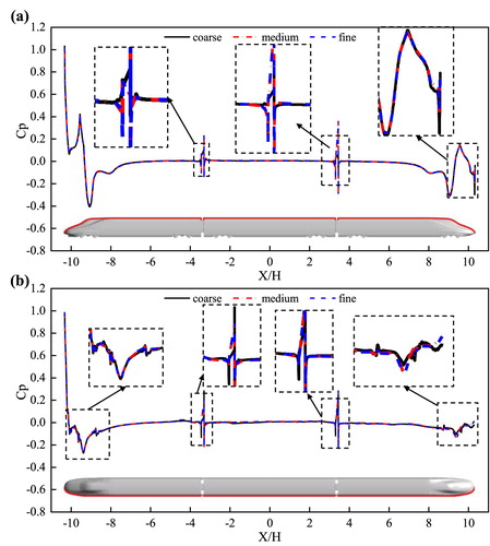
The distribution of $C_p$ on the train surface along the top symmetry line and the sideline of z = 0.27H for the three mesh densities were compared in Figure 6. As shown in Figure 6(a) and (b), $C_p$ along the symmetry line and sideline for three mesh densities basically coincided, except for the parts surrounding the inter-car gaps and streamlined zone of the tail car. The reason may be that the airflow in these regions is relatively complex and more sensitive to the mesh densities due to the complex geometry structures and flow separation, however, the difference between the medium and fine mesh is almost negligible.

Figure 6. Comparisons of the distribution of C_p of the train models with different mesh densities along different lines: (a) symmetry line of top surface and (b) side line along the horizontal section of z = 0.27H.

For the aerodynamic drag, the pressure drag over the head and tail car was dominant, and the next largest component is the skin friction drag over the train surfaces (Weinman et al., 2018). The pressure drag is determined by the pressure distribution on the HST model surface while the boundary layer thickness surrounding the HST model plays a decisive role in the viscous drag. Thus, it is necessary to analyze the influence of the mesh density on the thickness of boundary layer profiles.

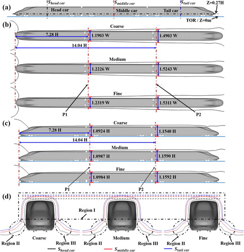
The distance normal from the train surface to where the velocity magnitude is 0.99$U_{inf}$ is termed as the boundary layer thickness, $\delta$ (Munson et al., 2009). Figure 7 shows $\delta$ profiles in different sections and the locations of these sections are depicted in Figure 7(a). The $\delta$ profile in the horizontal section of z = 0.27 H is revealed in Figure 7(b) and the distance between the two sides of $\delta$ profile at P1 and P2 were determined for easy quantitative comparison. Figure 7(b) indicates that the differences of these distances between the medium and fine mesh are only 0.75% and 0.44%, respectively. The distance between the $\delta$ profile in the symmetry section and the TOR (top of rail) also given at P1 and P2 in Figure 7(c), and the differences of these distances for the medium and fine mesh are almost negligible. Figure 7(d) shows the $\delta$ profiles in three cross sections, $S_{\text{head car}}$, $S_{\text{middle car}}$, and $S_{\text{tail car}}$, which are the middle sections of each vehicle from the head to tail car, respectively. Differences of $\delta$ profiles between the three different mesh densities appear in Regions II and III, with no significant difference in Region I. This may be because that Regions II and III are closer to the model train bottom flow region, where the flow field structure is more complex and more sensitive to mesh densities than it was in Region I. However, the differences of the $\delta$ profiles in these regions between the medium and fine mesh are very small and even negligible and the similar comparative validation has been also performed in other literature (Niu, Wang, Zhang, et al., 2018). According to the foregoing comparisons of the train aerodynamic quantities for three mesh densities, it can be concluded that the mesh with medium density is capable to accurately simulate the airflow around these train models. Thus, the following analysis data are based on the medium mesh.

Figure 7. Comparisons of the $\delta$ profiles for different sections of the train model with different mesh densities: (a) locations of different sections, (b) horizontal section of z = 0.27H, (c) symmetry section of y = 0, (d) middle sections of each single car.

3.2. Numerical method verification

A gap spacing of 8 mm was utilized in the wind tunnel experiment. Thus, aerodynamic quantities for the HST model with this gap spacing in this study were compared against the data from the wind tunnel experiment (Zhang, Yang, et al., 2018; Zhang & Zhou, 2013) to verify the reliability of the numerical algorithm. China Aerodynamics Research and Development Center has conducted the wind tunnel tests for a 1/8th three-car HST model, as revealed in Figure 2(a). The velocity of incoming airflows in the wind tunnel has been measured by a four-hole dynamic pressure probe (Cobra Probe 270) with a detecting accuracy of ±1 m/s in the range of ±45° cone angle, which has a sampling time and frequency of 15 s and 2 kHz, respectively. The aerodynamic resistance of each carriage model was measured separately by an independent box-type force balance with six components. For three force balances utilized by the head, middle and tail cars, the precision of the drag force are 0.05% and the accuracy are 0.15%, 0.13%, and 0.12%, respectively. The pressure distribution was measured by a pressure-scanning valves with a precision ±0.03%. Therefore, the test and measurement system had advantages of high precision and accuracy and the measured data is reliable. More relative details of the wind tunnel test were given in the report by (Zhang, Yang, et al., 2018).

As shown in Table 3, $C_x$ in this study was compared with that from the wind tunnel test and other numerical simulations based on different methods. $C_x$ in this study shows good agreement with wind tunnel experiment data, giving a maximal discrepancy of 3.7%, and has similar prediction accuracy compared with other numerical simulations. And as shown in Figure 8, $C_p$ along the symmetry centerline of the streamlined zones was also compared with the wind tunnel test (Gao et al., 2019; Zhang, Yang, et al., 2018). $C_p$ distribution in this study shows good consistency with the wind tunnel data. However, there is a small deviation of $C_p$ values at certain positions surrounding the nose of the tail car and the pressure value of the positive pressure region in the numerical simulation is larger than that in the wind tunnel test, which shows good consistency with the data in Table 3 that $C_x$ of the tail car in the numerical simulation is smaller than the corresponding wind tunnel data. The deviation is within the acceptable scope of the project; thus, the methodology is suitable for this study.

Figure 8. Comparisons of the pressure distributions on the symmetry line of the train between the experimental and numerical results.

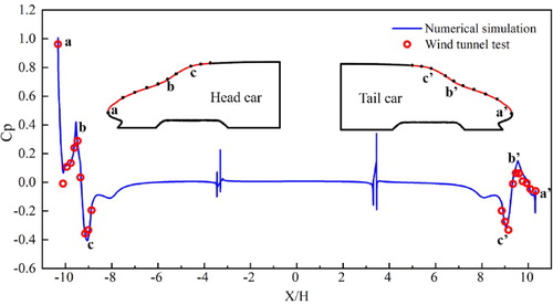
Table 3. Comparisons of drag coefficient between simulation and wind tunnel data.

	$C_x$
Methods	Cells	Head car	Middle car	Tail car
Numerical simulation (D = 8 mm)	47 million	0.146	0.078	0.157
Wind tunnel test (Zhang & Zhou, 2013)	–	0.145	–	0.163
DES (Zhang, Yang, et al., 2016)	16 million	0.144	0.081	0.160
IDDES (Niu et al., 2018)	25 million	0.1404	0.0764	0.1661
RANS (Gao et al., 2019)	41 million	0.139	0.078	0.153

4. Results and discussions

4.1. Analysis of the aerodynamic force

The existence of gap spacings directly affected the airflow surrounding two inter-car gap regions, and the gap spacing may have different influence on far-gap and near-gap parts due to the formation mechanism of aerodynamic drag. Table 4 shows the $C_x$ acting on far-gap and near-gap parts of the train models with different gap spacings, respectively.

Table 4. Aerodynamic drag coefficient $C_x$ acting on each part.

	Drag force coefficients $C_x$
Components	D = 0 mm	D = 5 mm	D = 8 mm	D = 10 mm	D = 20 mm	D = 30 mm
tc1	0.1639	0.1635	0.1635	0.1637	0.1637	0.1635
tc2	−0.0103	−0.0150	−0.0172	−0.0225	−0.0196	−0.0270
Head car	0.1536	0.1485	0.1463	0.1412	0.1441	0.1365
zc1	0.0572	0.0570	0.0571	0.0575	0.0575	0.0570
zc2	0.0183	0.0233	0.0286	0.0315	0.0278	0.0364
zc3	−0.0011	−0.0031	−0.0082	−0.0105	−0.0136	−0.0162
Middle car	0.0744	0.0772	0.0775	0.0785	0.0717	0.0772
wc1	0.1372	0.1367	0.1388	0.1429	0.1391	0.1395
wc2	0.0107	0.0121	0.0182	0.0206	0.0236	0.0265
Tail car	0.1479	0.1488	0.1570	0.1635	0.1627	0.1660
Total	0.3759	0.3745	0.3808	0.3832	0.3785	0.3797

Generally, when the near-gap part is upstream of the vehicle, the $C_x$ of the near-gap parts of each vehicle with different gap spacings are always positive. However, when the near-gap part is downstream of the vehicles, the $C_x$ are negative. Furthermore, regardless of whether the near-gap part is upstream or downstream of each vehicle, the absolute value of the $C_x$ acting on the near-gap parts generally tends to increase with the increase of gap spacings, which will be further elaborated by the pressure distribution in Figure 10. However, compared with the variation of the $C_x$ acting on the near-gap parts, the change of the gap spacing has no significant influence on the $C_x$ of the far-gap parts of each vehicle. For the $C_x$ of tc1 and zc1 (which are respectively the far-gap parts of the head and middle cars, respectively), the maximum deviations between the six different gap spacings are only 0.24% and 0.87%, respectively. This indicates that the impact of the gap spacing on the drag coefficients of tc1 and zc1 can nearly be neglected. The maximum deviation of the drag coefficient of wc1 between the six different gap spacings are 4.34%, which may have been because wc1 is located in the downstream region of these two inter-car gaps, and the structure change of airflow fields caused by the variation of the gap spacings has a more significant impact on the drag coefficient of wc1 compared with those of tc1 and zc1. However, this deviation was still very small compared with that of the near-gap part.

For all the gap spacings, tc2 and zc3 show negative drag coefficients, and the absolute value of the $C_x$ acting on zc3 gradually increases as the gap spacing increases. Similarly, absolute value of the $C_x$ of tc2 generally shows an increasing trend with the gap spacings except for the gap spacing of 20 mm. When the near-gap part is located at the upstream end of the vehicle such as zc2 and wc2, the $C_x$ acting on the near-gap part is positive for all six gap spacings. Upon increasing the gap spacing, the $C_x$ of wc2 shows an increasing tendency, and the $C_x$ of zc2 shows a general increasing trend, except that the drag coefficient for D = 20 mm is slightly smaller than that for D = 10 mm. This is similar to the tendency of the drag coefficient of tc2.

The above analysis shows that as the gap spacing varies, the $C_x$ of tc2 and zc2 as well as zc3 and wc2 both show similar trends. This occurs because tc2 and zc2 are located surrounding inter-car gap 1, whereas zc3 and wc2 are located around inter-car gap 2. The change in airflow structure surrounding the same inter-car gap region may have a similar influence on the two near-gap parts on both sides. The aerodynamic drag coefficient of the near-gap part shows different variation trends with the variation of the gap spacing, when near-gap parts are around different inter-car gap regions, and this is due to the different variations of the flow field structures in the different inter-car gaps.

For the head car, the total resistance coefficient decreases by 3.32%, 4.75%, 8.07%, 6.18%, and 11.13%, respectively, compared with the gap spacing of 0 mm, when the gap spacings are 5, 8, 10, 20, and 30 mm. While the total resistance coefficient increases by 0.61%, 6.15%, 10.55%, 10.01%, and 12.24%, respectively, with regard to the tail car. For the middle car, there are two near-gap parts on both ends of the middle car (i.e. zc2 and zc3). zc2 is the upstream end of the middle car, which experiences a positive drag, whereas zc3 is the downstream end, which experiences a negative drag. Due to the drag variation of the near-gap parts caused by the gap spacing variation, the positive and negative drag variations offset to some extent. Therefore, for the middle car, the variation of the total resistance coefficient is not as significant as those of the other two cars. The maximum deviation of the total drag coefficient of the middle car is only 5.51% compared with the gap spacing of 0 mm, which occurs when the gap spacing is 10 mm. For the overall HST model resistance, the gap spacing of 5 mm decreases by 0.37%, whereas the gap spacing of 8, 10, 20, and 30 mm increases by 1.30%, 1.94%, 0.69%, and 1.01%, respectively, compared with the drag coefficient for the gap spacing of 0 mm. And the variation of the aerodynamic drag with gap spacings is different from the results from other literature (Li et al., 2019) to some extent, which may be due to two reasons: one is the discrepancy of the internal and external windshield structures studied, and the other is the different ways to obtain different gap spacings.

4.2. Analysis of train surface pressure distribution

The $C_p$ on the HST model surfaces is used to better understand the effect of the D value, because the pressure difference force over the train dominates the aerodynamic forces (Weinman et al., 2018). Thus, combined with the result and analysis in Table 4, in this section, analysis of the $C_p$ on the train model surfaces is conducted, based on the numerical simulation results for the train models with gap spacings of 0, 8, 20, and 30 mm, respectively. The $C_p$ along the centerlines of the top surface of train models, which are also the profiles of models’ x-z symmetrical planes, are shown and analyzed in Figure 9.

Figure 9. Comparisons of the pressure coefficient distribution along the centerlines of the top surfaces of the train models.

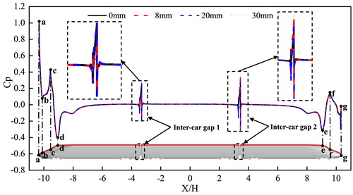
In general, the $C_p$ curves for four cases with different gap spacings are almost consistent, except at the positions in the regions near inter-car gap 1 and inter-car gap 2. As shown in Figure 9, small differences in the $C_p$ amplitudes can be found near the two inter-car gap regions. When the position of the upper centerline is located at the downstream end wall surfaces of the head and middle car, there is a negative pressure in these positions, whereas there is a positive pressure in the positions located at the upstream end wall surfaces of the middle and tail car. This occurs because the air flow flowing along the train surface undergoes flow separation at the inter-car gap regions due to the discontinuous surface, which is further analyzed in Figure 10. The above analyses show that the variations of the gap spacing has no significant influence on the $C_p$ profile along the centerline of the HST model top surface, except the positions surrounding two inter-car gap regions. A similar case of the bogie cut-outs’ angles of the high-speed train also demonstrated a similar observation (Zhang, Yang, et al., 2018).

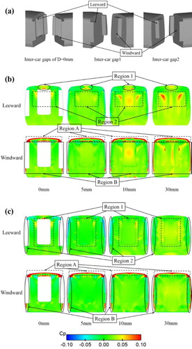
Figure 10. Comparisons of the pressure coefficient distribution: (a) geometry diagram of the leeward and windward end walls, (b) leeward and windward end walls of inter-car gap1, (c) leeward and windward end walls of inter-car gap2.

The above analysis also shows that the variations of the gap spacing directly affects the $C_p$ on the train surface near the inter-car gap regions. Therefore, the $C_p$ on the surface in the two inter-car gap regions will be further analyzed to investigate the effect of the gap spacing in detail. As shown in Figure 2, there are two inter-car gaps in each train model, called inter-car gap 1 and inter-car gap 2. The two sides of inter-car gap 1 are the end wall of the head car and the upstream end wall of the middle car, called the leeward end wall surface and windward end wall surface, respectively. Similarly, for inter-car gap 2, the leeward end wall surface is the downstream end wall of the middle car, and the windward end wall surface is the end wall of the tail car. Figure 10(a) shows the geometric structures of the leeward and windward end walls of the inter-car gap in the train models with different gap spacings. When the gap spacing is 0 mm, inter-car gap1 and inter-car gap2 have the same geometric structures for the leeward and windward end walls. Thus, only one geometry diagram of inter-car gaps is shown. For the train model with the other five gap spacings, the geometric structures of the leeward and windward end walls of inter-car gap1 are different from those of inter-car gap2. Thus, both geometric structure diagrams are given for inter-car gap1 and inter-car gap2.

Figure 10(b) and (c) show the $C_p$ distributions on the leeward and windward end wall surfaces of inter-car gap 1 and inter-car gap 2, respectively, for gap spacings of 0, 5, 10, and 30 mm. For inter-car gap1, the $C_p$ distribution on the end wall of HST model surfaces is almost symmetric about the span-wise mid-plane due to the absence of crosswinds. There are two significant positive pressure regions on the leeward end wall, i.e. region 1 and region 2, and two significant positive pressure regions on the windward end wall, i.e. region A and region B. Region 1 and region A are located near the top region of inter-car gap 1. Thus, the $C_p$ on these two regions are mainly determined by the airflow structure around the top region of inter-car gap 1. As the gap spacing increases, the positive pressure area in region A shows no significant variation, whereas that in region 1 decreases slightly. This occurs because a groove structure region is formed between the top surface of the internal windshield and two end wall surfaces of the two adjacent vehicle bodies. The airflow flowing along the train top surface enters the groove structure due to the flow separation, directly impacting region A, after which it flows back along the top surface of the internal windshield to form a vortex and finally impacts region 1 on the leeward side. With the increase of the gap spacing, the thickness of the internal windshield decreases, and the airflow flowing back along the top surface of the internal windshield impacts region 1 at a lower speed. However, the top geometric structure of the groove region does not change with the gap spacing, and thus the airflow almost impacts region A with the same speed. Region 2 and region B are mainly located in the region near the middle of inter-car gap 1. As the gap spacing increases, the airflow flowing along the top and side surface of the train enters the middle region of inter-car gap 1 at a higher speed. These airflows with higher velocities are possibly slowed down due to the stagnation of regions 2 and B, which causes a higher pressure on these regions. The reason for these variations is further elaborated by the analysis of the flow filed structure, as shown in Figure 11(b).

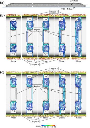
Figure 11. Comparisons of the tangential component of the velocity in the z = 0.562H plane: (a) z = 0.562H plane position diagram; (b) inter-car gap 1; (c) inter-car gap2.

For inter-car gap2, the positive pressure areas of the leeward and windward end walls are smaller than those of the leeward and windward end walls of inter-car gap1. This occurs because when the airflow flows from upstream to downstream along the train top surface, due to the existence of viscous shear stresses between the airflow and train surface, the airflow velocity on the train surface gradually decreases, which is further validated by the analysis of the tangential component of the velocity vector and the boundary layer thickness, as shown in Figures 11 and 13.

The variation of the pressure in region 1 is similar to that in region 2 of inter-car gap1. In region 2, i.e. the external windshield region on the side of the train, when the gap spacing is 5 mm, there is a small negative pressure area. The negative pressure region gradually disappears and becomes a positive pressure area, as the gap spacing increases. When the gap spacing is small, the airflow entering the gap from the side of the inter-car gap because of flow separations forms small vortices in the gap around the external windshields, which leads to the negative pressure in region 2. When the gap spacing gradually increases, the airflow due to the flow separation flowing into the inter-car gap from the side flows smoothly into region 1, and little vortex formed near Region 2. The pressure variations with the gap spacing of regions A and B is similar to those of region A and region B in inter-car gap1.

4.3. Airflow structure around the HST model

Pressure distributions on the HST model surface are mainly determined by the airflow field around the train models. The above analysis shows that the gap spacing significantly affects pressure distributions on the HST model surface surrounding inter-car gap 1 and inter-car gap 2. To further research the effect of the gap spacing on the airflow structures around two inter-car gap regions, the airflow characteristics surrounding two inter-car gaps of the HST models with gap spacings of 0, 5, 8, 20, and 30 mm will be analyzed in this section.

As depicted in Figure 11, the tangential component of the velocity vector in the z = 0.562 H plane are compared. Figure 11(b) demonstrates the tangential velocity component around inter-car gap 1, and the airflow field surrounding the inter-car gap 1 mainly contains three regions, region 1, 2, and 3. Regions 1 and 3 are between the end walls of the head and middle car bodies, and flow structures around these two regions are almost symmetric about the longitudinal section of the train model because the geometric structure around the two regions are symmetric about the longitudinal section and there is no crosswind. As the gap spacing increases, the airflow along the train surface flows into the region 1 more smoothly and with a higher speed, because the kinetic energy loss of the airflow due to the geometric structure obstruction is reduced. The higher velocity airflow flowing into region 1 forms a main vertex with a higher speed. During the rotation of the vortex, the airflow at the edge of the vortex impacts the end wall surface of the train body at a higher speed. This further demonstrates the variation of the pressure coefficient distribution with the gap spacing shown in Figure 10(b).

Region 2 contains the zone between the end walls of the internal windshield of the head car and the end wall of the middle car. With the change of the gap spacing, the flow structure in region 2 shows a significant variation. When the gap spacing is 0 mm, region 2 does not exist. As the gap spacing gradually increases, the airflow contained in region 2 increases significantly. However, when the gap spacing is smaller than 8 mm, the airflow in region 2 is very low. When the gap spacing reaches 20 mm, high-velocity airflow occurs in region 2. The high-speed airflow in region 2 gradually forms small vertices when the gap spacing is 30 mm. This significantly affects the pressure distribution of the surface near region 2, which is also shown in Figure 10(b). With the change of the gap spacing, the variations of the airflow structure in regions 1, 2, and 3 of inter-car gap 2 is similar to those of inter-car gap 1. These differences in airflow structures surrounding inter-car gap 1 for the different gap spacings are more significant compared with those around inter-car gap 2, which can be confirmed by Figure 10.

The skin friction drag over the train, as an important part of the aerodynamic resistance acting on HSTs, mainly depends on the thickness of boundary layer surrounding trains. Thus, researching the influence of gap spacings on the boundary layer thickness is essential. Figure 12(b) shows the boundary layer thickness in the two sections for all of the gap spacings. The locations of section 1 and section 2 is given in Figure 12(a). Section 1 is 0.067 H from the windward end wall of inter-car gap 1. Similarly, the distance between section 2 and the windward end wall of inter-car gap 2 is 0.067 H. The boundary layers at the same sections in the six different cases almost have a similar contour shape. Furthermore, the boundary layer thickness in section 1 is significantly larger than that in section 2 in all of the cases, i.e. the boundary layer profile gradually becomes thicker from upstream to downstream of HST model, similar to results obtained by (Zhang, Wang, et al., 2018). This further clarifies why the high-pressure region on the windward and leeward end wall of gap 1 is always larger than that of gap 2.

Figure 12. Boundary layer around the train model with six different gap spacings: (a) positions of the sections, (b) boundary layer thickness in two sections for all cases.

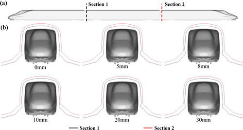
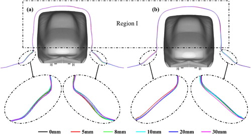
Figure 13 compares the boundary layer thicknesses for all the cases in the same section. In all the cases, the boundary layer thicknesses of sections 1 and 2 in region I are almost the same, whereas there are some discrepancies in the boundary layer profile surrounding six HST model with different gap spacings in the regions below region I and the similar phenomenon could be found in the report of Gao et al. (2019). In these regions below region I, the discrepancy in the boundary layer profile in section 1 are significantly greater than those in section 2. In section 2, when the gap spacing increases up to 30 mm, there is a small discrepancy in the boundary layer profile compared with the other cases. For the boundary layer profile on section 1, when the gap spacing is less than 10 mm, there is basically no difference between cases with gap spacings of 0, 5, and 8 mm. However, there is a small discrepancy when the gap spacing is 10 mm compared with the smaller gap spacings, and when the gap reaches 20 mm or 30 mm, the discrepancies are more significant compared with the cases with smaller gap spacings. This result shows that the airflow structures near inter-car gap 1 are more sensitive to the variation of the gap spacings and show more significant discrepancies of flow structure between cases with different gap spacings compared to those near inter-car gap 2. This is also evident in the analysis of the variation of the pressure coefficient distribution and velocity vectors in Figures 10 and 11, respectively. This may be because the thickness of boundary layer profile near inter-car gap 1 is thinner compared with that near inter-car gap 2, and the airflow surrounding inter-car gap 1 has a higher velocity.

Figure 13. Boundary layers in the two different sections of the train: (a) section 1 and (b) section 2.

5. Conclusion and future work

In this study, numerical simulations of HST models scaled at 1/8th based on RANS were carried out to research the influence of the gap spacing between adjacent vehicles on the aerodynamic forces, pressure distribution, and airflow structure surrounding the HST models. The summary of the main results of this study are shown below:

1. The gap spacing between adjacent vehicles affects the airflow structure surrounding the HST model and changes the train surface pressure distribution, which eventually leads to significant differences in the aerodynamic resistance of each train carriage.

2. The gap spacing has more significant influence on the drag coefficient of the near-gap parts than that of the far-gap part. The gap spacing can significantly lessen the aerodynamic resistance acting on the head car and increase that acting on the tail car, whereas the variation of the total drag acting on the middle car is not as large as that of the head and tail cars. When the gap spacing reaches 30 mm, the discrepancies of the aerodynamic resistance of the head and tail cars reach the maximum value, which is 11.13% and 12.24%, respectively, compared with those for the gap spacing of 0 mm. However, compared with the gap spacing of 0 mm, the maximum difference of the total drag coefficient of the entire train model is smaller than 2.0%. When the gap spacing is not greater than 8 mm, the discrepancies of the aerodynamic resistance coefficients of the head, middle, and tail cars do not exceed 6.15%, compared with those for the gap spacing of 0 mm.

3. As the gap spacing increases, the variations of the pressure distribution on the train surface, airflow structure, and boundary layer thickness in the region around inter-car gap 1 are more significant compared with those surrounding inter-car gap 2.

This study investigated the influence of gap spacing on aerodynamic performances and flow field structures of the high-speed train model at zero yaw angle, however, some yaw angles beyond zero were also considered during wind tunnel experiments. The gap spacings may have some different effects on HST models under other yaw angles. Future studies will mainly focus on the effect of the gap spacings on the aerodynamic performances of the HST models with crosswinds in the wind tunnel tests.

Acknowledgements

The authors acknowledge the computational resources provided by the High-Speed Train Research Centre of Central South University, China.

Disclosure statement

No potential conflict of interest was reported by the author(s).

Additional information

Funding

This work was supported by the National Key R&D Program of China [grant number 2016YFB1200504] and the National Natural Science Foundation of China [grant number 51575538].

References

- Akbarian, E., Najafi, B., Jafari, M., Faizollahzadeh Ardabili, S., Shamshirband, S., & Chau, K.-W. (2018). Experimental and computational fluid dynamics-based numerical simulation of using natural gas in a dual-fueled diesel engine. Engineering Applications of Computational Fluid Mechanics, 12(1), 517–534. https://doi.org/10.1080/19942060.2018.1472670
- ANSYS Inc. (2017). ANSYS fluent user’s guide.
- Baker, C. J. (2014a). A review of train aerodynamics part 2 – Applications. Aeronautical Journal, 118(1202), 345–382. https://doi.org/10.1017/S0001924000009179 doi: 10.1017/S0001924000009179
- Baker, C. J. (2014b). A review of train aerodynamics: Part 1 – Fundamentals. Aeronautical Journal, 118(1201), 201–228. https://doi.org/10.1017/S000192400000909X doi: 10.1017/S000192400000909X
- Bell, J. R., Burton, D., Thompson, M., Herbst, A., & Sheridan, J. (2014). Wind tunnel analysis of the slipstream and wake of a high-speed train. Journal of Wind Engineering and Industrial Aerodynamics, 134, 122–138. https://doi.org/10.1016/j.jweia.2014.09.004 doi: 10.1016/j.jweia.2014.09.004
- Bocciolone, M., Cheli, F., Corradi, R., Muggiasca, S., & Tomasini, G. (2008). Crosswind action on rail vehicles: Wind tunnel experimental analyses. Journal of Wind Engineering and Industrial Aerodynamics, 96(5), 584–610. https://doi.org/10.1016/j.jweia.2008.02.030 doi: 10.1016/j.jweia.2008.02.030
- Brockie, N. J. W., & Baker, C. J. (1990). The aerodynamic drag of high speed trains. Journal of Wind Engineering and Industrial Aerodynamics, 34(3), 273–290. https://doi.org/10.1016/0167-6105(90)90156-7
- CEN European Standard 14067-4, C. E. S. (2010). Railway applications-aerodynamics. Part 4: Requirements and test procedures for aerodynamics on open track.
- Chen, G., Li, X.-B., Liu, Z., Zhou, D., Wang, Z., Liang, X.-F., & Krajnovic, S. (2019). Dynamic analysis of the effect of nose length on train aerodynamic performance. Journal of Wind Engineering and Industrial Aerodynamics, 184, 198–208. https://doi.org/10.1016/j.jweia.2018.11.021 doi: 10.1016/j.jweia.2018.11.021
- Gao, G., Li, F., He, K., Wang, J., Zhang, J., & Miao, X. (2019). Investigation of bogie positions on the aerodynamic drag and near wake structure of a high-speed train. Journal of Wind Engineering and Industrial Aerodynamics, 185, 41–53. https://doi.org/10.1016/j.jweia.2018.10.012 doi: 10.1016/j.jweia.2018.10.012
- Ghalandari, M., Bornassi, S., Shamshirband, S., Mosavi, A., & Chau, K. W. (2019). Investigation of submerged structures’ flexibility on sloshing frequency using a boundary element method and finite element analysis. Engineering Applications of Computational Fluid Mechanics, 13(1), 519–528. https://doi.org/10.1080/19942060.2019.1619197 doi: 10.1080/19942060.2019.1619197
- He, X., Zhou, L., Chen, Z., Jing, H., Zou, Y., & Wu, T. (2019). Effect of wind barriers on the flow field and aerodynamic forces of a train–bridge system. Proceedings of the Institution of Mechanical Engineers, Part F: Journal of Rail and Rapid Transit, 233(3), 283–297. https://doi.org/10.1177/0954409718793220 doi: 10.1177/0954409718793220
- Kurec, K., Remer, M., Mayer, T., Tudruj, S., & Piechna, J. (2019). Flow control for a car-mounted rear wing. International Journal of Mechanical Sciences, 152, 384–399. https://doi.org/10.1016/j.ijmecsci.2018.12.034 doi: 10.1016/j.ijmecsci.2018.12.034
- Kurec, K., Remer, M., & Piechna, J. (2019). The influence of different aerodynamic setups on enhancing a sports car’s braking. International Journal of Mechanical Sciences, 164, 105140. https://doi.org/10.1016/j.ijmecsci.2019.105140 doi: 10.1016/j.ijmecsci.2019.105140
- Kwon, H. B., Park, Y. W., Lee, D. H., & Kim, M. S. (2001). Wind tunnel experiments on Korean high-speed trains using various ground simulation techniques. Journal of Wind Engineering and Industrial Aerodynamics, 89(13), 1179–1195. https://doi.org/10.1016/S0167-6105(01)00107-6 doi: 10.1016/S0167-6105(01)00107-6
- Li, T., Hemida, H., Zhang, J., Rashidi, M., & Flynn, D. (2018). Comparisons of shear stress transport and detached eddy simulations of the flow around trains. Journal of Fluids Engineering, 140(11), 111108–111112. https://doi.org/10.1115/1.4040672
- Li, T., Li, M., Wang, Z., & Zhang, J. (2019). Effect of the inter-car gap length on the aerodynamic characteristics of a high-speed train. Proceedings of the Institution of Mechanical Engineers, Part F: Journal of Rail and Rapid Transit, 233(4), 448–465. https://doi.org/10.1177/0954409718799809 doi: 10.1177/0954409718799809
- Liu, T.-H., Jiang, Z.-H., Li, W.-H., Guo, Z.-J., Chen, X.-D., Chen, Z.-W., & Krajnovic, S. (2019). Differences in aerodynamic effects when trains with different marshalling forms and lengths enter a tunnel. Tunnelling and Underground Space Technology, 84, 70–81. https://doi.org/10.1016/j.tust.2018.10.016
- Menter, F. R. (1994). Two-equation eddy-viscosity turbulence models for engineering applications. AIAA Journal, 32(8), 1598–1605. https://doi.org/10.2514/3.12149 doi: 10.2514/3.12149
- Menter, F. R., Kuntz, M., & Langtry, R. (2003). Ten years of industrial experience with the SST turbulence model. Turbulence, Heat and Mass Transfer, 4, 625–632.
- Morden, J. A., Hemida, H., & Baker, C. J. (2015). Comparison of RANS and detached eddy simulation results to wind-tunnel data for the surface pressures upon a class 43 high-speed train. Journal of Fluids Engineering, 137(4), 512. https://doi.org/10.1115/1.4029261 doi: 10.1115/1.4029261
- Mou, B., He, B.-J., Zhao, D.-X., & Chau, K.-W. (2017). Numerical simulation of the effects of building dimensional variation on wind pressure distribution. Engineering Applications of Computational Fluid Mechanics, 11(1), 293–309. https://doi.org/10.1080/19942060.2017.1281845 doi: 10.1080/19942060.2017.1281845
- Munoz-Paniagua, J., García, J., & Lehugeur, B. (2017). Evaluation of RANS, SAS and IDDES models for the simulation of the flow around a high-speed train subjected to crosswind. Journal of Wind Engineering and Industrial Aerodynamics, 171, 50–66. https://doi.org/10.1016/j.jweia.2017.09.006 doi: 10.1016/j.jweia.2017.09.006
- Munson, B. R., Young, D. F., Okiishi, T. H., & Huebsch, W. W. (2009). Fundamentals of fluid mechanics (sixth ed.). Don Fowley.
- Niu, J., Liang, X., & Zhou, D. (2016). Experimental study on the effect of Reynolds number on aerodynamic performance of high-speed train with and without yaw angle. Journal of Wind Engineering and Industrial Aerodynamics, 157, 36–46. https://doi.org/10.1016/j.jweia.2016.08.007 doi: 10.1016/j.jweia.2016.08.007
- Niu, J., Wang, Y., Liu, F., & Li, R. (2020). Numerical study on the effect of a downstream braking plate on the detailed flow field and unsteady aerodynamic characteristics of an upstream braking plate with or without a crosswind. Vehicle System Dynamics, 3(11), 1–18. https://doi.org/10.1080/00423114.2019.1708959 doi: 10.1080/00423114.2019.1708959
- Niu, J., Wang, Y., Zhang, L., & Yuan, Y. (2018). Numerical analysis of aerodynamic characteristics of high-speed train with different train nose lengths. International Journal of Heat and Mass Transfer, 127, 188–199. https://doi.org/10.1016/j.ijheatmasstransfer.2018.08.041 doi: 10.1016/j.ijheatmasstransfer.2018.08.041
- Niu, J., Zhou, D., & Liang, X.-F. (2018). Numerical simulation of the effects of obstacle deflectors on the aerodynamic performance of stationary high-speed trains at two yaw angles. Proceedings of the Institution of Mechanical Engineers, Part F: Journal of Rail and Rapid Transit, 232(3), 913–927. https://doi.org/10.1177/0954409717701786 doi: 10.1177/0954409717701786
- Niu, J., Zhou, D., & Liang, X. (2018). Numerical investigation of the aerodynamic characteristics of high-speed trains of different lengths under crosswind with or without windbreaks. Engineering Applications of Computational Fluid Mechanics, 12(1), 195–215. https://doi.org/10.1080/19942060.2017.1390786
- Niu, J., Zhou, D., Liang, X.-F., Liu, S., & Liu, T.-H. (2018). Numerical simulation of the Reynolds number effect on the aerodynamic pressure in tunnels. Journal of Wind Engineering and Industrial Aerodynamics, 173, 187–198. https://doi.org/10.1016/j.jweia.2017.12.013 doi: 10.1016/j.jweia.2017.12.013
- Raghunathan, R. S., Kim, H. D., & Setoguchi, T. (2002). Aerodynamics of high-speed railway train. Progress in Aerospace Sciences, 38(6-7), 469–514. https://doi.org/10.1016/S0376-0421(02)00029-5
- Rahman, M. M., Vuorinen, V., Taghinia, J., & Larmi, M. (2018). Wall-distance-free formulation for SST k–ω model. European Journal of Mechanics – B/Fluids, 75, 71–82. https://doi.org/10.1016/j.euromechflu.2018.11.010 doi: 10.1016/j.euromechflu.2018.11.010
- Raina, A., Harmain, G. A., & Haq, M. I. U. (2017). Numerical investigation of flow around a 3D bluff body using deflector plate. International Journal of Mechanical Sciences, 131-132, 701–711. https://doi.org/10.1016/j.ijmecsci.2017.08.018 doi: 10.1016/j.ijmecsci.2017.08.018
- Schober, M., Weise, M., Orellano, A., Deeg, P., & Wetzel, W. (2010). Wind tunnel investigation of an ICE 3 endcar on three standard ground scenarios. Journal of Wind Engineering and Industrial Aerodynamics, 98(6-7), 345–352. https://doi.org/10.1016/j.jweia.2009.12.004 doi: 10.1016/j.jweia.2009.12.004
- Sicot, C., Deliancourt, F., Boree, J., Aguinaga, S., & Bouchet, J. P. (2018). Representativeness of geometrical details during wind tunnel tests. Application to train aerodynamics in crosswind conditions. Journal of Wind Engineering and Industrial Aerodynamics, 177, 186–196. https://doi.org/10.1016/j.jweia.2018.01.040
- Versteeg, H. K., & Malalasekera, W. (2007). An introduction to computational fluid dynamics: The finite volume method (second ed.). Pearson Education Ltd.
- Weinman, K. A., Fragner, M., Deiterding, R., Heine, D., Fey, U., Braenstroem, F., & Wagner, C. (2018). Assessment of the mesh refinement influence on the computed flow-fields about a model train in comparison with wind tunnel measurements.
- Willemsen, E. (1997). High Reynolds number wind tunnel experiments on trains. Journal of Wind Engineering and Industrial Aerodynamics, 69–71, https://doi.org/10.1016/S0167-6105(97)00175-X
- Xia, C., Shan, X., & Yang, Z. (2016). Comparison of different ground simulation systems on the flow around a high-speed train. Proceedings of the Institution of Mechanical Engineers, Part F: Journal of Rail and Rapid Transit, 231, 2. https://doi.org/10.1177/0954409715626191.
- Xiang, H., Li, Y., Chen, S., & Li, C. (2017). A wind tunnel test method on aerodynamic characteristics of moving vehicles under crosswinds. Journal of Wind Engineering and Industrial Aerodynamics, 163, 15–23. https://doi.org/10.1016/j.jweia.2017.01.013
- Zhang, J., Li, J.-J., Tian, H.-Q., Gao, G.-J., & Sheridan, J. (2016). Impact of ground and wheel boundary conditions on numerical simulation of the high-speed train aerodynamic performance. Journal of Fluids and Structures, 61, 249–261. https://doi.org/10.1016/j.jfluidstructs.2015.10.006 doi: 10.1016/j.jfluidstructs.2015.10.006
- Zhang, J., Wang, J., Wang, Q., Xiong, X., & Gao, G. (2018). A study of the influence of bogie cut outs’ angles on the aerodynamic performance of a high-speed train. Journal of Wind Engineering and Industrial Aerodynamics, 175, 153–168. https://doi.org/10.1016/j.jweia.2018.01.041 doi: 10.1016/j.jweia.2018.01.041
- Zhang, L., Yang, M.-Z., & Liang, X.-F. (2018). Experimental study on the effect of wind angles on pressure distribution of train streamlined zone and train aerodynamic forces. Journal of Wind Engineering and Industrial Aerodynamics, 174. https://doi.org/10.1016/j.jweia.2018.01.024 doi: 10.1016/j.jweia.2018.01.024
- Zhang, Z., & Zhou, D. (2013). Wind tunnel experiment on aerodynamic characteristic of streamline head of high speed train with different head shapes. Journal of Central South University (Science and Technology), 44(6), 2603–2608.