Numerical simulation of wind turbulence by DSRFG and identification of the aerodynamic admittance of bridge decks

Abstract

Discretizing and synthesizing random flow generation (DSRFG) is applied to generate inflow turbulence satisfying large eddy simulation (LES) requirements for bridge wind engineering. The variation of the turbulent wind along the computational domain is investigated considering multiple grid sizes and time steps. The aerodynamic admittance functions (AAFs) of a thin plate and two bridge sections are evaluated. Turbulence properties are well maintained from the inlet downstream in the windward direction. The grid resolution minorly affects the along-wind profiles of the mean velocity and turbulence intensity, but it greatly influences the wind spectra. The turbulence energy of the wind spectra may decay in the high-frequency range, which can be improved by applying finer grids and small time steps. Reasonable grid and time step size are suggested to provide stable turbulent wind flow along the computational domain. Fairly good agreement between the estimated AAFs of the thin plate and the Sears function validate the feasibility of LES in predicting the AAFs. The AAFs of the bridge sections are different from the Sears function. The contributions of the longitudinal and vertical velocity components to the buffeting forces are not equal, and it is inappropriate to employ one equivalent AAF for each force component.

KEYWORDS:

• Bridge engineering
• large eddy simulation
• box girder
• DSRFG
• aerodynamic admittance function

1. Introduction

A rapid increase in the development of transportation may require the construction of super long-span bridges using high-strength and light-weight materials. As a result, such flexible and low-damped structures will be more sensitive to natural wind, and large-amplitude vibration may be observed under strong wind conditions. Hence, the reasonable prediction of wind-induced structural behavior, such as the buffeting response under turbulent wind, is critical in the design of long-span bridges to ensure structural safety and serviceability. Historically, the design and study of the wind resistance of long-span bridges has been mainly based on wind tunnel tests, which are widely recognized as the most reliable and effective way to investigate the behavior of structures under natural wind conditions. However, the necessary test equipment and instruments are costly, and carrying out such wind tunnel testing is time-consuming. In the application of computational fluid dynamics (CFD) to bridge wind engineering, the governing equations of the air flow around the bridge are numerically solved in the computational domain with prescribed boundary conditions. Hence, the accuracy of the CFD simulation will be greatly affected by the applied boundary conditions, especially when turbulent flow is considered.

Buffeting is a kind of stochastic vibration with limited amplitude under turbulent flow. The aerodynamic admittance function (AAF) was first introduced by Davenport (1962) to describe the relationship between the inflow turbulence and the aerodynamic forces acting on the structure. To date, the Sears function (Sears, 1941) is the only analytic solution of the AAF and is derived from a sinusoidal gust wind acting on a thin airfoil. However, the Sears function fails to represent the buffering forces of bluff bridge decks due to the occurrence of complex flow separation and reattachment. The AAFs of a bridge deck depend on the geometry of the girder section and the inflow turbulence, which should be identified through wind tunnel tests. According to traditional buffeting theory, there are six aerodynamic admittance components, i.e. ${\chi }_{Fa}$ (F = D_b, L_b, M_b; a = u, w), where D_b, L_b, and M_b are the buffeting lift force, drag force and torsional moment, respectively, and u and w are the longitudinal and vertical velocity components, respectively. Due to the inherent difficulty in distinguishing the coupled contribution from the velocity components u and w, the equivalent AAF method has been widely used, in which ${\chi }_{Fu}={\chi }_{Fw}={\chi }_F$ is assumed. The AAF of a bridge deck is the relation between the auto spectrum of the buffeting force $S_{FF}$ and the velocity component $S_{aa}$. The buffeting forces can be measured by pressure measurements (Larose & Mann, 1998; Ma et al., 2019) or force-balance measurements (Gu & Qin, 2004; Larose, 1999; Matsuda et al., 1999). To identify all six AAF components, many researchers have carried out extensive research over the past several years. Li (2007) proposed an unsteady model that could reflect the influence of turbulent fluctuations on the gust load components, in which the six AAF components were explicitly defined. By assuming that the AAFs are not sensitive to the wind angle of attack within a very small range, Chen et al. (2009) proposed a zero-separation method to identify six AAF components. Han et al. (2010) proposed a separated frequency-by-frequency method to identify the six AAF components using an active turbulence generator in a wind tunnel. Zhao and Ge (2015) estimated the AAF components by considering the cross-PSD functions between the forces and the turbulence components. Zhu et al. (2018) identified the six AAF components of bridge decks by applying the colligated residue least squares method of auto – and cross-spectra (CRLSMACS).

Currently, wind tunnel tests are widely recognized as an effective way to identify the AAFs of bridge decks. In these tests, force or pressure measurements are carried out in turbulent flow. However, wind tunnel testing requires special equipment, instruments and model fabrication, making it costly and time-consuming. Furthermore, the AAFs of bridge decks are sensitive to the ratio between the length scale of gusts and the deck width (Larose & Mann, 1998). It is difficult to simulate the length scale of natural gusts in wind tunnels. Although CFD is widely used to evaluate static wind loads (Li et al., 2019; Mou et al., 2017; Salih et al., 2019), vortex-induced forces (Chen et al., 2018) and self-excited aerodynamic forces (Ghalandari et al., 2019; Zhu et al., 2007), the identification of the AAFs of bridge decks with CFD has rarely been reported. In recent years, some attempts at such work have been carried out using CFD. Bruno et al. (2005) numerically simulated the AAFs of streamlined and bluff bodies using the RNG $k-\epsilon$ model and LES, respectively. They found that the effect of the signature turbulence was dominant and that the AAFs were strongly sensitive to the inlet flow conditions. Uejima et al. (2008) evaluated AAFs of basic cross sections under vertical wind gusts by the two dimensional $k-\omega$ SST model. The results showed that flow separation had a great influence on the performance of the AAFs, i.e. the AAF of a bridge deck depends on its cross section. Rasmussen et al. (2010) and Hejlesen et al. (2015) simulated the AAFs of bluff bodies using discrete vortex method. The computed results agreed well with the available experimental data. Most, numerical simulations of AAFs of bridge decks have been based on two-dimensional simulations, which cannot represent the three-dimensional characteristics of inflow turbulence. Furthermore, the AAFs of bridge decks are sensitive to inflow turbulence, and it is necessary to generate a turbulent wind field satisfying the wind characteristics of the bridge site.

Turbulent flow is a complicated fluid motion that is highly random, unsteady, three-dimensional and time-dependent. The length and time scales of turbulent flow are sufficiently broad to make CFD simulation very challenging to execute (Ferziger & Peric, 2002). Currently, LES is widely used to simulate turbulent flow fields (Liu et al., 2018; Naimul Haque, et al., 2014). The main challenge in the LES is to provide a turbulent wind field that satisfies the prescribed statistical characteristics at the inlet boundary. The detailed properties of the oncoming flow have a significant effect on the aerodynamic performance of the simulated body. Precursor simulation method and synthesis method are two basic methods to generate the inflow boundary condition. The precursor simulation method usually includes a pre-computation to generate inflow fluctuations as a database, which is then introduced into the inlet of the main computational domain. Inflow fluctuations generated by the precursor simulation method are compatible with the Navier-Stokes equations and possess accurate turbulence information, requiring only a relatively short transition distance to achieve a fully developed state. However, the computational costs of the precursor simulation method are considerable, and it is difficult to modify the turbulence properties, which makes it difficult to apply to engineering applications. Another type of method widely used to generate inflow boundary conditions is the synthesis method. The synthesis method attempts to construct random fluctuations with prescribed turbulent properties, and then the generated fluctuations are added to the mean velocity profile. Hoshiya (1972) proposed a spectral method to generate multi-correlated random velocities satisfying the prescribed power spectral density (PSD) and cross-spectral density. However, the generated inflow turbulence does not satisfy the divergence-free condition, which may affect the convergence of LES. Kondo et al. (1997) applied a divergence-free operation to make the generated turbulence satisfy the divergence-free condition. To avoid undesirable influences caused by grid skewness, a stringent restriction should be imposed on the time step for the divergence-free operation. Because the inflow fluctuations are generated based on cross-spectral density of different points, the generation process is not independent for each point. Therefore, the spectral methods described above are not appropriate to implement parallel computing. Kraichnan (1970) developed a variant of the spectral method to generate an isotropic turbulent flow with a specified energy spectrum. This method was carried out by synthesizing the velocity field as a set of Fourier components. However, it fails to represent the inhomogeneity and anisotropy of the turbulent flow field. Random flow generation (RFG) was proposed by Smirnov et al. (2001) based on Kraichnan’s method, which introduces the length and time scales of turbulence. The turbulent flow field generated by the RFG method is divergence-free for homogeneous turbulence and high-degree divergence-free for inhomogeneous turbulence. Batten et al. (2004) proposed a simplified alternative to the RFG method. To replace the similarity transformations in the RFG method, an additional tensor scaling is introduced to account for turbulence anisotropy. Notably, the turbulent flow fields generated by the methods of Smirnov et al. (2001) and Batten et al. (2004) follow Gaussian’s spectral model, which deviates from a realistic wind spectrum. To generate inflow turbulence satisfying any given spectrum, Huang et al. (2010) developed the DSRFG method based on Kraichnan’s method. The continuous spectrum is discretized into a series of segments, and the turbulence fluctuations are generated by Kraichnan’s method for each segment. Aligning and remapping procedures are adopted to account for the inhomogeneity and anisotropy of the turbulent flow field. The DSRFG method can strictly guarantee divergence-free condition, and it is suitable for parallel computation. Some modifications to the DSRFG method were made by Castro and Paz (2013) and Aboshosha et al. (2015), who proposed the MDSRFG method and the CDRFG, respectively. Other synthesis methods include proper orthogonal decomposition method, digital filter method and vortex method. Descriptions of these methods can be found in reviews of turbulent flow generation methods by Tabor and Baba-Ahmadi (2010) and Dhamankar et al. (2018). In general, the synthesis method is more robust than the precursor simulation method because it does not require costly prior simulations, and it is convenient to specify and modify the turbulence parameters if conditions change.

In the present study, the AAFs of a flat plate, a streamlined box girder (Great Belt East Bridge) and a $\mathrm{\Pi }$ type girder (Danjiang Reservoir Bridge) are investigated by three-dimensional LES. To simulate a realistic turbulent wind field, the DSRFG method is applied to generate inflow turbulence with the wind characteristics of the Great Belt East Bridge site. Notably, the inflow turbulence generated by the synthesis method guarantees only the continuity equation, rather than the complete Navier-Stokes equations. Therefore, a fairly long adaptation region should be set between the inlet boundary and the object so that the inflow turbulence can achieve a fully developed state. With the influence of the LES model, the grid arrangement and the time step size, the turbulent properties of the inflow turbulence are likely to change. Few studies have been conducted to investigate the variation of the inflow turbulence in the computational domain. In this study, the generated inflow turbulence is introduced to the inlet of the computational domain applying user-defined functions in the commercial software Fluent. The impacts of the grid resolution and the computational time step on the variation of the turbulent properties along the computational domain are investigated, and reasonable grid and time step sizes are suggested to provide a stable turbulent wind field.

2. Numerical method

2.1. Governing equations

For incompressible flow, the governing equations of LES can be expressed in the Cartesian coordinate system as follows (Ferziger & Peric, 2002) (1) $\begin{array}{rl}& \frac{\mathrm{\partial }{\overline{u}}_i}{\mathrm{\partial }{x}_i}=0\end{array}$(1) (2) $\begin{array}{rl}& \frac{\mathrm{\partial }{\overline{u}}_i}{\mathrm{\partial }t}+\frac{\mathrm{\partial }{\overline{u}}_i{\overline{u}}_j}{\mathrm{\partial }{x}_j}=-\frac{1}{\rho }\frac{\mathrm{\partial }\overline{p}}{\mathrm{\partial }{x}_i}+\upsilon \frac{{\mathrm{\partial }}^2{\overline{u}}_i}{\mathrm{\partial }{x}_i\mathrm{\partial }{x}_i}-\frac{1}{\rho }\frac{\mathrm{\partial }{\tau }_{ij}}{\mathrm{\partial }{x}_j}\end{array}$(2) where ${\overline{u}}_i$ and $\overline{p}$ are the filtered velocity and pressure, respectively; $\rho$ is the density; $\upsilon$ denotes the kinematic viscosity; $x_i$ is the coordinate in space; ${\tau }_{ij}$ is the subgrid-scale stress, which can be defined as (3) ${\tau }_{ij}=-2{\mu }_t{\overline{S}}_{ij}+\frac{1}{3}{\tau }_{kk}{\delta }_{ij};{\overline{S}}_{ij}=\frac{1}{2}\left(\frac{\mathrm{\partial }{\overline{u}}_i}{\mathrm{\partial }{x}_j}+\frac{\mathrm{\partial }{\overline{u}}_j}{\mathrm{\partial }{x}_i}\right)$(3) where ${\mu }_t$ and ${\overline{S}}_{ij}$ are the eddy-viscosity and the strain rate of resolved scale, respectively; $\delta$ is the Kronecker function. In the Smagorinsky-Lilly model, ${\mu }_t$ can be modeled by (4) ${\mu }_t=\rho L_s^2|\overline{S}|=\rho L_s\sqrt{2{\overline{S}}_{ij}{\overline{S}}_{ij}};L_s=min(\kappa d,C_s\mathrm{\Delta })$(4) where $\kappa$ is the von Karman constant, $\kappa =0.42$; d is the distance to the closest wall; $\mathrm{\Delta }$ is the local grid scale; C_s is the Smagorinsky constant equal to 0.1.

2.2. Review of the DSRFG technique

A brief review of the DSRFG technique is performed in the present study, more details about the DSRFG method can be found in the work of Huang et al. (2010). According to the DSRFG method, the turbulent flow field u(x,t) can be synthesized as follows: (5) $\begin{array}{rl}{u}_i(\mathbf{\text{x}},t)& =\sum _{m=1}^M\sum _{n=1}^N[p_i^{m,n}\cos (k_j^{\mathrm{\prime }m,n}{x^{\mathrm{\prime }}}_j+{\omega }_{m,n}t)\\ & +q_i^{m,n}\sin (k_j^{\mathrm{\prime }m,n}{x^{\mathrm{\prime }}}_j+{\omega }_{m,n}t)]\end{array}$(5) where (6) $\begin{array}{rl}& p_i^{m,n}=\text{sign}(r_i^{m,n})\sqrt{\frac{4}{N}{E}_i(k_m)\frac{{(r_i^{m,n})}^2}{1+{(r_i^{m,n})}^2}}\end{array}$(6) (7) $\begin{array}{rl}& q_i^{m,n}=\text{sign}(r_i^{m,n})\sqrt{\frac{4}{N}{E}_i(k_m)\frac{1}{1+{(r_i^{m,n})}^2}}\end{array}$(7) (8) $\begin{array}{rl}& k_j^{\mathrm{\prime }m,n}=k_j^{m,n}/k_0\end{array}$(8) (9) $\begin{array}{rl}& x_j^{\mathrm{\prime }}=x_j/l_s\end{array}$(9) (10) $\begin{array}{rl}& {\omega }_{m,n}\in N(0,2\pi f_m),f_m=k_m{U}_0\end{array}$(10) where M and N are the numbers of discrete spectrum segments and harmonic components, respectively; k is wavenumber, and $k_0$ is the lowest wavenumber; t is the time; $l_s$ is the scale factor; f is the frequency; $U_0$ is the mean velocity; $r_i^{m,n}$ is random number selected independently from a three-dimensional normal distribution with a mean of 0 and a standard deviation of 1; sign is the sign function. The wavenumber vector $k_j^{m,n}$ determines the distribution of the energy spectrum function $E(k)$ in space, which can be defined as: (11) $\begin{array}{rl}& {\mathbf{\text{k}}}^{m,n}\cdot {\mathbf{\text{p}}}^{m,n}=0\end{array}$(11) (12) $\begin{array}{rl}& {\mathbf{\text{k}}}^{m,n}\cdot {\mathbf{\text{q}}}^{m,n}=0\end{array}$(12) (13) $\begin{array}{rl}& |{\mathbf{\text{k}}}^{m,n}|=k_m\end{array}$(13)

The inflow boundary condition for the LES can be attained by introducing u(x,t) to the mean profile. It is essential to ensure that the synthesized fluctuations satisfy the divergence-free condition; otherwise, the turbulent fluctuations may redistribute and dissipate quickly (Patruno & Ricci, 2017; Tabor & Baba-Ahmadi, 2010). As Huang et al. (2010) noted, the inflow fluctuations generated by the DSRFG method strictly satisfy the divergence-free condition and any desired target spectrum. Notably, the target spatial correlation can be attained by adjusting the value of l_s. Most importantly, the turbulence generation process at a point on the inlet surface is independent of the turbulence generation processes at all other points. Therefore, it is convenient to implement parallel computing.

3. Numerical application

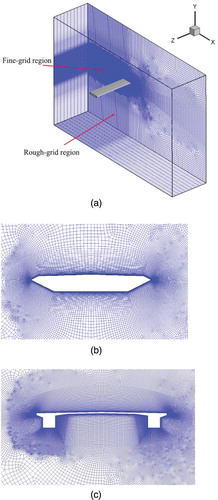
The bridge sections investigated in the present study are shown in Figure 1. The girder attachments are ignored, and only the bridge deck in the construction stage is considered in the CFD simulations. The length scale of the bridge girder is 1/80. The arrangement of the computational domain is shown in Figure 2. The distance between the inlet boundary and the girder shear center is 2 m, which is approximately 5B (where B is the width of the model), and the distance from the girder shear center to the upper or to the lower boundaries is also 5B. Therefore, the blockage ratio is 1.4%, which is less than the recommended blockage ratio in wind engineering applications (Tominaga et al., 2008). The outlet boundary is 4 m from the girder shear center, which is a distance of approximately 10B. The girder length in the spanwise direction is 0.5B. The computational domain is generated by combining structured and unstructured hexahedral meshes, as shown in Figure 3(a). Finer mesh is used near the box girder and in regions between the inlet boundary and the girder, whereas coarser mesh is used in regions far from the box girder. As shown in Figure 3(b) and (c), mapped mesh is generated around the deck, and the height of the wall-adjacent cell is set to 1.3 × 10⁻⁵B. Unstructured cells are paved in the buffer zone connecting the fine-grid region and rough-grid region, helping ensure good control of the mesh quantity. The stretching ratio of adjacent grids in the computational domain is less than 1.1.

Figure 1. Cross-sections of bridge decks: (a) Great Belt East Bridge, (b) Danjiang Reservoir Bridge (units: m).

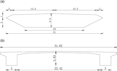
Figure 2. Computational domain and boundary conditions.

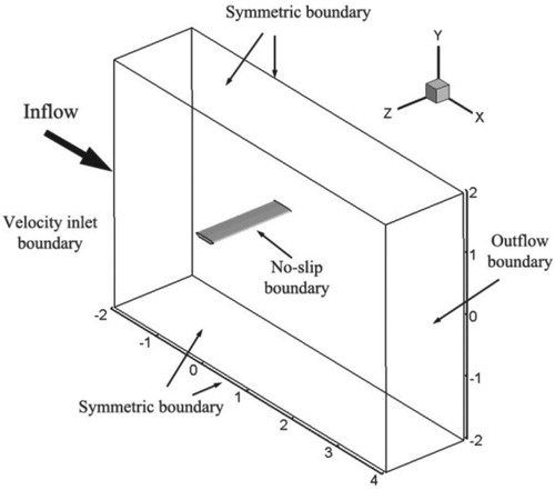
Figure 3. Meshing of the computational domain: (a) overview of the mesh arrangement, (b) distribution of the mesh near the streamlined box girder, (c) distribution of the mesh near the $\mathrm{\Pi }$ type girder.

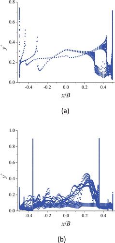
The boundary conditions of the computational domain are shown in Figure 2. The velocity inlet boundary is used for the inlet of the computational domain. The upper and lower boundaries, as well as the spanwise boundaries, are all specified as symmetric boundaries. The outflow boundary condition is applied to the model flow exits, where a zero diffusion flux is assumed at the exit. Wall boundary conditions are used at the girder surface. The mean wind speed of 10 m/s is specified at the inlet, and the corresponding Reynolds number is 2.7 × 10⁵. The distribution of y+ on the girder surface is shown in Figure 4. It is found that y+ values of wall-adjacent cells are all less than 1, which meets the requirement of the LES.

Figure 4. y⁺ distribution on girder surface: (a) Great Belt East Bridge, (b) Danjiang Reservoir Bridge.

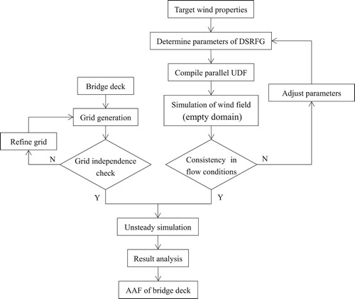
The workflow for the identification of the AAF of bridge decks is shown in Figure 5. The numerical simulations are performed based on the commercial code Fluent. The initial field is established by running a steady-state flow simulation, in which the standard $k-\epsilon$ model with the first-order scheme is adopted. When the flow field is reasonably converged, the LES is enabled. The momentum term and the unsteady term are discretized by the bounded central differencing scheme, and the second-order implicit scheme, respectively. The pressure-velocity coupling scheme is the semi-implicit pressure-linked equations consistent (SIMPLEC) algorithm.

Figure 5. Workflow for the identification of the AAF of bridge decks.

4. Numerical simulation of the wind field

4.1. Generation of inflow turbulence

The energy content of the turbulent wind field is described by its PSD, so it is important to ensure that the inflow turbulence satisfies a realistic wind spectrum. The von Karman spectral model has been generally accepted as the commonly used analytical representation of the atmospheric boundary layer. The expressions of the von Karman spectral equations are described as follows (Simiu & Scanlan, 1996): (14) $\begin{array}{rl}{S}_u(f)& =\frac{4{(I_u{U}_0)}^2(L_u/U_0)}{{[1+70.8{(f{L}_u/U_0)}^2]}^{5/6}}\end{array}$(14) (15) $\begin{array}{rl}{S}_v(f)& =\frac{4{(I_v{U}_0)}^2(L_v/U_0)(1+188.4{(2f(L_v/U_0))}^2)}{{[1+70.8{(2f{L}_v/U_0)}^2]}^{11/6}}\end{array}$(15) (16) $\begin{array}{rl}{S}_w(f)& =\frac{4{(I_w{U}_0)}^2(L_w/U_0)(1+188.4{(2f(L_w/U_0))}^2)}{{[1+70.8{(2f{L}_w/U_0)}^2]}^{11/6}}\end{array}$(16) where S_i, I_i and L_i (i = u, v, w) are the wind spectra, turbulence intensity and integral length scales, respectively; u, v and w are the longitudinal, transverse and vertical velocity components, respectively. The turbulence properties of the Great Belt East Bridge site are adopted to generate inflow turbulence, as shown in Table 1 (Larsen, 1993). The lateral turbulence intensity I_v is assumed to be 0.88I_u. Generally, the integral length scale simulated in a wind tunnel is below 1 m, and the longitudinal integral length scale L_u in the present study is assumed to be 0.5 m. L_v and L_w are assumed to be 0.25L_u and 0.1L_u, respectively (Solari & Piccardo, 2001). The coherence function is approximated by the Davenport exponential form (17) ${\gamma }_u^y(f)=\text{exp}\left(\frac{-2\alpha f\mathrm{\Delta }y}{U_0}\right)$(17) where $\alpha$ is the exponential decay factor equal to 8. $\mathrm{\Delta }y$ is the separation of reference stations along the lateral direction. Target spatial correlations are given by (Hémon & Santi, 2007) (18) $\begin{array}{rl}S{c}_{i,j}& =\sum _l\sqrt{S_{u,i}(f_l)S_{u,j}(f_l)}{\gamma }_u^y(f_l)\\ & =\sum _l\sqrt{S_{u,i}(f_l)S_{u,j}(f_l)}exp\left(\frac{-2\alpha |y_i-y_j|f_l}{U_0}\right)\end{array}$(18)

Table 1. Turbulence properties at the Great Belt East Bridge site.

Longitudinal turbulence intensity	Iu	10%
Vertical turbulence intensity	Iw	6%
Exponential decay factor	α	8

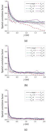
The scale factor ls is used to adjust the spatial correlation of inflow turbulence, which can be defined as (19) $l_s=C_{sp}\sqrt{L_u^2+L_v^2+L_w^2}$(19) where $C_{sp}$ is a constant. Huang et al. (2010) suggested a value of $C_{sp}$ between 1 and 2. Comparison of the spatial correlations for different $C_{sp}$ with the target ones are presented in Figure 6. The results show that the simulated spatial correlations agree well with the target ones when $C_{sp}$ is 5, while the spatial correlations are underestimated when $C_{sp}$ is between 1 and 2. Therefore, the value of $C_{sp}$ should be determined by the prescribed spatial correlations.

Figure 6. Comparison of the spatial correlation factors with different C_sp values: (a) u component, (b) v component, (c) w component.

The key parameters adopted to generate inflow turbulence are presented in Table 2, where dt is the time step size. Figure 7 shows the samples of simulated fluctuating velocity generated by the DSRFG method. The standard deviation values of each velocity component are compared with the target values in Table 3, where ${\sigma }_u$, ${\sigma }_v$ and ${\sigma }_w$ are the standard deviation values of the longitudinal, transverse and vertical velocity components, respectively. The relative error of the simulated value is within 4%, indicating that the turbulence intensity of the inflow turbulence agrees well with the prescribed value. The spectra of the velocity components are presented in Figure 8. It is found that the simulated spectra agree well with the target von Karman spectral model throughout the frequency range. As demonstrated above, the DSRFG method can generate turbulent flow in accordance with specified statistical characteristics.

Figure 7. Simulated time histories of fluctuating wind velocity.

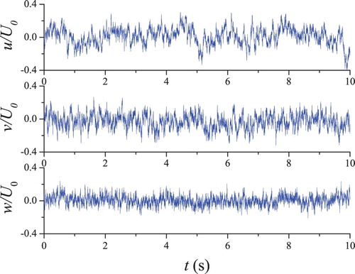
Figure 8. Simulated wind spectra in comparison with target spectra.

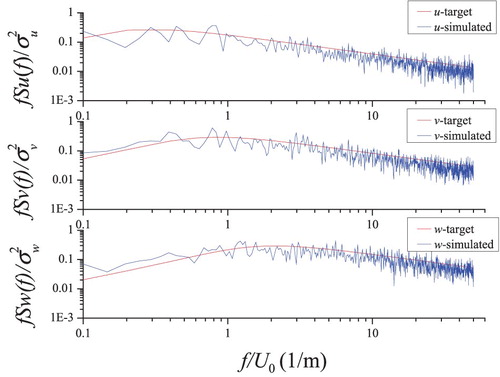
Table 2. Key parameters adopted in the DSRFG method.

M	N	dt	Csp
256	100	0.001s	5

Table 3. Simulated turbulent velocities for Great Belt East Bridge site in comparison with target values.

	Target value	Simulated value	Relative error
σu	1	1.011	1.1%
σv	0.88	0.873	0.8%
σw	0.6	0.577	3.8%

4.2. Simulation of a wind field

The identification of AAFs of structures is strongly dependent on the wind field, so the correct simulation of wind fields is an important prerequisite. The LES of an empty computational domain (without the box girder) is conducted to investigate the variation of the inflow turbulence in the computational domain. In CFD simulation, the DSRFG method is programmed based on C Language as a user-defined function in Fluent software. During the simulation, this self-developed code is first loaded and solved by Fluent to generate turbulent wind data at each element center at the inlet boundary on each time step. The generated wind data impose on their corresponding cell centers on the inlet boundary of the computational domain, and the LES simulation is carried out on this time step.

4.2.1. Grid resolution

An empty computational domain (without the box girder) is established with the same computational domain size and boundary conditions described in section 3. The gird size ($\mathrm{\Delta }l$) of the horizontal and vertical grids are identical in the fine-grid zone. To study the impacts of the grid size on the characteristics of the inflow turbulence, three cases with different grid resolutions in the fine-grid region were simulated, i.e. 0.5, 1 and 2 cm. With the exception of the grid resolution in the fine-grid region, the other simulation conditions remained the same. To obtain the pattern of variation in the turbulent wind at the height of the bridge axis along the computational domain, the history of velocities was recorded by setting monitoring points at several cross sections (x = 0, −0.5, −1, −1.5 and −2 m).

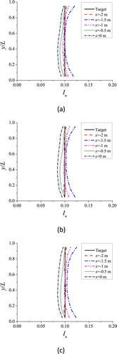
Based on the simulated results, the comparisons of the simulated mean velocity profiles with the target profile are shown in Figure 9, where $U_m$ is the mean simulated velocity. As expected, the simulated mean velocity profiles are similar from the inlet to the downstream, and all profiles at various locations are consistent with the target profile. Figure 10 shows the comparisons of the turbulence intensity profiles with the target profile. It is found that the simulated results provide reasonable agreement with the target profile. However, the simulated results slightly underestimate the turbulence intensity in the range from x = −0.5 m to x = 0 m. The major reason for the difference should be the filtering effect of the mesh and the numerical viscosity of the turbulence model. The present results show no distinct difference between the results of the simulated profiles obtained by employing different grid sizes, indicating that the grid sizes investigated have little influence on the mean velocity and turbulence intensity. It is found that both the mean velocity and turbulence intensity are slightly overestimated near the spanwise boundaries, where the symmetric boundary conditions are employed. Therefore, in order to avoid the influence from the boundaries, it is suggested to set a larger computational domain, such as increase the girder length in spanwise direction.

Figure 9. Mean wind velocity profiles in comparison with target profiles: (a) $\mathrm{\Delta }l$=2 cm, (b) $\mathrm{\Delta }l$=1 cm, (c) $\mathrm{\Delta }l$=0.5 cm.

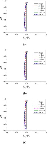
Figure 10. Turbulence intensity profiles in comparison with target profiles: (a) $\mathrm{\Delta }l$=2 cm, (b) $\mathrm{\Delta }l$=1 cm, (c) $\mathrm{\Delta }l$=0.5 cm.

The accurate simulation of the realistic turbulence spectra of the wind flow field in the frequency range of interest is important in the field of wind engineering, particularly in assessing dynamic effects induced by the wind at or near the natural frequency of a structure. Here, the time histories of the fluctuating velocities are recorded, and a spectral analysis is carried out. Welch's overlapped segment averaging estimator is adopted to obtain a PSD estimate of the fluctuating velocity. Figure 11 shows the spectra of the longitudinal velocity component for three grid sizes. The simulated spectra, especially the spectrum at $x=0$, are in acceptable agreement with the target spectrum. This agreement indicates that the spectra of the generated wind flow field satisfy a realistic turbulence spectrum model and the dynamics of eddy motions are well reproduced by the DSRFG method. Notably, the energy of the high-frequency range decays. 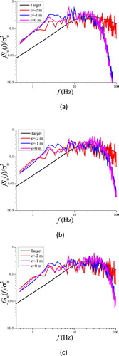In particular, for the coarsest grid level ($\mathrm{\Delta }l$ = 2 cm), the energy decays significantly as the frequency exceeds 25 Hz. This phenomenon can be improved by applying finer grids. As shown in Figure 11(b) and Figure 11(c), the simulated spectra match the target spectrum well with a wider range of frequencies when finer grids are applied. This result indicates that a finer grid resolution results in more features of the turbulence being captured in the high-frequency range. Therefore, the grid size should be selected carefully so that the simulated wind flow field can accurately represent the features of turbulence in the frequency range of interest. Figure 12 shows the spectra of the vertical velocity component for three grid sizes. The simulated spectra are slightly overestimated at low frequencies.

Figure 11. Spectra of the longitudinal velocity component in comparison with the target spectrum: (a) $\mathrm{\Delta }l$=2 cm, (b) $\mathrm{\Delta }l$=1 cm, (c) $\mathrm{\Delta }l$=0.5 cm.

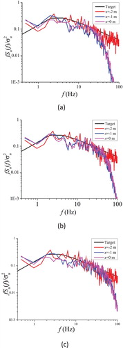
Figure 12. Spectra of the vertical velocity component in comparison with the target spectrum: (a) $\mathrm{\Delta }l$=2 cm, (b) $\mathrm{\Delta }l$=1 cm, (c) $\mathrm{\Delta }l$=0.5 cm.

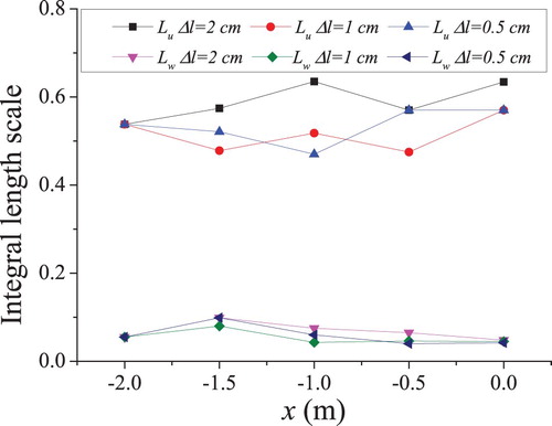
If the simulated spectra match the von Karman spectrum, the integral length scale can be determined as follows (Flay & Stevenson, 1988): (20) $\begin{array}{rl}{L}_u& =0.146U_0/n_p\end{array}$(20) (21) $\begin{array}{rl}{L}_w& =0.106U_0/n_p\end{array}$(21) where $n_p$ is the frequency corresponding to the peak of the spectrum. Figure 13 shows the simulated integral length scales in the computational domain. Although considerable discreteness is observed for different grid sizes, the simulated integral length scales are in acceptable agreement with the target, indicating that the average size of eddy motions is reasonably reproduced by the DSRFG method.

Figure 13. Turbulence integral scales in the computational domain.

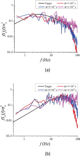
4.2.2. Time step size

As Huang et al. (2010) noted, the time step size dt is a key parameter in the DSRFG method, and the computational cost of the DSRFG method is f_max times that of the RFG method, where $f_{max}=1/(2dt)$. Hence, it is essential to choose a reasonable time step size to reduce the computational cost. The inflow turbulence is generated by adopting dt = 0.001 s, while dt used in the LES is different from that of the DSRFG method. Therefore, inflow fluctuations should be interpolated in the time dimension before application to the inflow boundary conditions. To study the impacts of dt used in LES on the characteristics of the inflow turbulence, three cases with different dt values are simulated, i.e. 1 × 10⁻³ s, 5 × 10⁻⁴ s and 1 × 10⁻⁴ s. With the exception of the time step, the other simulation conditions remain the same, and a grid system with a resolution of 1 cm in the fine-grid region is used. Figure 14 presents the simulated spectra at x = 0 m for three time step sizes. The results show that the spectrum in the high-frequency range has much better consistency with the target spectrum when a smaller dt is used.

Figure 14. Wind spectra at x=2 m with different time step sizes in comparison with the target spectrum: (a) Spectra of the longitudinal velocity component, (b) Spectra of the vertical velocity component.

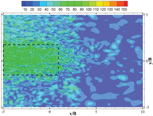
According to the above observations, the statistical turbulence properties of the simulated wind field provide reasonable agreement with the target properties, implying the turbulence achieves a fully developed and stable state. Considering reasonable accuracy and computational cost, it is suggested that a grid system with a resolution of 1 cm in the fine-grid region and dt  = 1 × 10⁻⁴ s can provide a reasonable turbulent wind field. To show the turbulence flow patterns of the flow, instantaneous turbulence kinetic energy contours and vorticity magnitude contours are plotted in Figures 15 and 16, respectively. Clearly, the turbulent flow field generated by DSRFG can reproduce large – and small-scale turbulent structures. The dashed rectangle shows the fine-grid region. It is found that more detailed turbulent structures are captured in the fine-grid region than in the rough-grid region.

Figure 15. Turbulence kinetic energy contours.

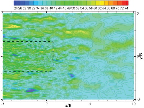
Figure 16. Vorticity magnitude contours.

5. Aerodynamic admittance

In the present study, the six AAF components of the model can be obtained using the following expressions (Li, 2007): (22) $\begin{array}{rl}{\chi }_{Lu}(K)& =\frac{S_w(K)S_{uL}(K)-S_{wu}(K)S_{wL}(K)}{\rho U_{0}b[S_u(K)S_w(K)-S_{wu}(K)S_{uw}(K)]}\end{array}$(22) (23) $\begin{array}{rl}{\chi }_{Lw}(K)& =\frac{S_u(K)S_{wL}(K)-S_{uw}(K)S_{uL}(K)}{\rho U_{0}b[S_u(K)S_w(K)-S_{uw}(K)S_{wu}(K)]}\end{array}$(23) (24) $\begin{array}{rl}{\chi }_{Du}(K)& =\frac{S_w(K)S_{uD}(K)-S_{wu}(K)S_{wD}(K)}{\rho U_{0}b[S_u(K)S_w(K)-S_{wu}(K)S_{uw}(K)]}\end{array}$(24) (25) $\begin{array}{rl}{\chi }_{Dw}(K)& =\frac{S_u(K)S_{wD}(K)-S_{uw}(K)S_{uD}(K)}{\rho U_{0}b[S_u(K)S_w(K)-S_{uw}(K)S_{wu}(K)]}\end{array}$(25) (26) $\begin{array}{rl}{\chi }_{Mu}(K)& =\frac{S_w(K)S_{uM}(K)-S_{wu}(K)S_{wM}(K)}{\rho U_0{b}^2[S_u(K)S_w(K)-S_{wu}(K)S_{uw}(K)]}\end{array}$(26) (27) $\begin{array}{rl}{\chi }_{Mw}(K)& =\frac{S_u(K)S_{wM}(K)-S_{uw}(K)S_{uM}(K)}{\rho U_0{b}^2[S_u(K)S_w(K)-S_{uw}(K)S_{wu}(K)]}\end{array}$(27) where $K=\omega B/U_0$; $\omega$ is the circular frequency; S_aF (a = u, w; F = D_b, L_b, M_b) is the cross-spectra between the fluctuating wind velocity and the buffeting force; S_uw and S_wu are the cross-spectra between the velocity component u and w, respectively; and b = B/2.

When the cross-spectrum between velocity component u and w is neglected, i.e. S_uw= S_wu = 0, Equations (22)–(27) can be simplified as follows: (28) $\begin{array}{rl}{\chi }_{Lu}(K)& =\frac{S_{uL}(K)}{\rho Ub{S}_u(K)}\end{array}$(28) (29) $\begin{array}{rl}{\chi }_{Lw}(K)& =\frac{S_{wL}(K)}{\rho Ub{S}_w(K)}\end{array}$(29) (30) $\begin{array}{rl}{\chi }_{Du}(K)& =\frac{S_{uD}(K)}{\rho Ub{S}_u(K)}\end{array}$(30) (31) $\begin{array}{rl}{\chi }_{Dw}(K)& =\frac{S_{wD}(K)}{\rho Ub{S}_w(K)}\end{array}$(31) (32) $\begin{array}{rl}{\chi }_{Mu}(K)& =\frac{S_{uM}(K)}{\rho U{b}^2{S}_u(K)}\end{array}$(32) (33) $\begin{array}{rl}{\chi }_{Mw}(K)& =\frac{S_{wM}(K)}{\rho U{b}^2{S}_w(K)}\end{array}$(33)

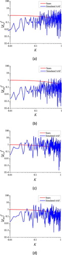
5.1. Aerodynamic admittance of a thin plate

Compared with a bridge deck, a thin plate is a relatively simple model, and the AAFs of a thin plate can be described by the Sears function. Hence, this simplified model can be a suitable benchmark to verify the effectiveness and applicability of numerical simulations of AAF. To evaluate the performance of the LES, the AAF of a thin plate is investigated before this approach is applied to the bridge girder section.

Liepmann’s approximation (Liepmann, 1952) of the Sears function is the most commonly used and is expressed as (34) $|\chi (k^{\mathrm{\prime }}){|}^2=\frac{1}{1+2\pi k^{\mathrm{\prime }}}$(34) where $k^{\mathrm{\prime }}=f\pi B/U_0$ is non-dimensional parameter.

The inflow turbulence described in section 4.1 around a thin plate with a plate thickness D = B/22.5 is simulated by LES. The time histories of the velocities and buffeting forces are recorded simultaneously. When sampling the velocity series 1B upstream of the leading edge, neither the thin plate section nor the bridge girder section has a significant influence on the turbulence properties of the sampled velocities. Since the Sears function is used to describe the unsteady characteristics of the buffeting lift force and torsional moment, the AAFs related to the buffeting drag force will not be discussed here. Figure 17 shows the AAFs of the thin plate under zero wind attack angle. It is found that $|{\chi }_{Lw}{|}^2$ obtained from the numerical simulations are in reasonable agreement with the Sears function, which indicates that the LES is a feasible method for predicting the AAFs. However, some deviations have been observed. In the low-reduced frequency range the identified values of $|{\chi }_{Lw}{|}^2$, especially those of $|{\chi }_{Mw}{|}^2$, are slightly below those of the Sears function. The observed deviations may be caused by the ‘strip assumption’ adopted by the Sears function, which neglects the turbulent characteristics of the incident flow and assumes that the turbulence length scale of the inflow turbulence is adequately larger than the characteristic length of the bluff body. Since the characteristic length of the thin plate is close to the turbulence length scale, the spatial correlation of the turbulent fluctuations reduces the identified AAFs. The Sears function is often applied to describe the AAF of a thin airfoil or a thin plate relating to the vertical velocity component. As shown in Figure 17, the AAF components relating to the longitudinal velocity component are generally lower than those of the Sears function, especially in the low-reduced frequency range. Therefore, it is necessary to distinguish the contribution from the velocity component u and w.

Figure 17. AAFs of a thin plate, (a) $|{\chi }_{Lu}{|}^2$, (b) $|{\chi }_{Mu}{|}^2$, (c) $|{\chi }_{Lw}{|}^2$ (d) $|{\chi }_{Mw}{|}^2$.

5.2. Aerodynamic admittance of the bridge decks

5.2.1. Pressure distribution of bridge decks

The arrangements of monitoring points on the surface of the bridge decks are shown in Figure 18, which are used to record the time histories of fluctuating pressures. The dimensionless pressure coefficients C_p can be defined as (35) $C_p=(P-P_0)/(0.5\rho U_0^2)$(35) where P and P₀ are static pressure and reference pressure, respectively.

Figure 18. Arrangement of the monitoring points: (a) Great Belt East Bridge, (b) Danjiang Reservoir Bridge.

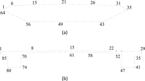
Figure 19(a) and (b) shows the distribution of the simulated pressure coefficients of the Great Belt East Bridge together with available results of wind tunnel tests (Larose, 1992; Zhu et al., 2016). The numerical results show overall good agreement with those of the section model study (Zhu et al., 2016). Obvious differences are found in the windward air fairing between the present simulation and the data measured on a taut strip model (Larose, 1992), which is probably due to the differences in the turbulent flow between the experiment and simulation. Figure 20(a) shows the instantaneous pressure contours around the streamlined box girder section. It is clear that positive pressures are concentrated near the windward fairing and that sharp negative values are distributed around the windward corners. Sharp negative values are also observed in the wake, which are caused by vortex shedding. Figure 21(a) shows the streamlines of the flow around the streamlined box girder section. The flow is intercepted by the presence of the girder section, and no obvious separation is observed around the leading edges. The flow divides at the corner of fairing, where the pressure is the maximum positive value. The flow is accelerated along the webs of the box girder, and the pressure energy is converted into kinetic energy, which leads to a pressure drop and a negative downward pressure. The pressures at point 6 and point 56 have the maximum negative values. The negative peak value is −1.22 (point 56). The flow is decelerated downstream along the top and bottom flanges, and this leads to the recovery of pressure. The flow separates near the corners on the leeward side, and a series of vortexes are formed near the trailing edges, creating negative pressure zones. The vortexes then shed form the trailing edges and form the wake flow downstream.

Figure 19. Mean pressure distribution, (a) upper surface of the Great Belt East Bridge, (b) lower surface of the Great Belt East Bridge, (c) Danjiang Reservoir Bridge.

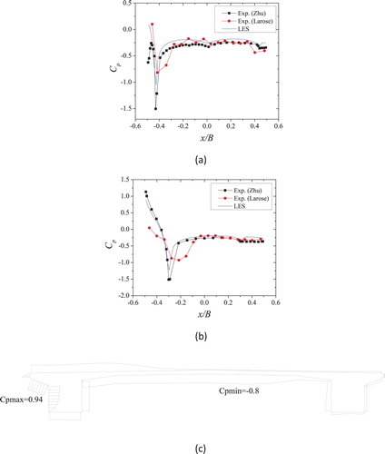
Figure 20. Instantaneous pressure contours around girder section: (a) Great Belt East Bridge, (b) Danjiang Reservoir Bridge.

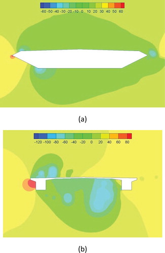
Figure 21. Streamlines of flow around the girder section: (a) Great Belt East Bridge, (b) Danjiang Reservoir Bridge.

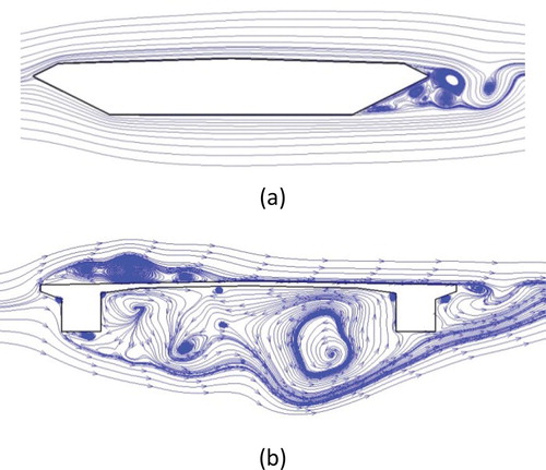
As for the Danjiang Reservoir Bridge, the mean pressure coefficients are shown in Figure 19(c). The positive pressures are presented by filled areas, while empty areas indicate negative pressures. It is found that positive pressure is concentrated on the leading edges, and the maximum pressure coefficient is 0.94 (point 85). Sharp negative pressures are observed on the upper surface in the windward side and the lower surface between two boxes, and the negative peak value is −0.8 (point 58). Figure 20(b) and Figure 21(b) show the instantaneous pressure contours and the streamlines of the flow around the girder section, respectively. Obvious separation is observed on the upper surface around the leading edge, and a large recirculation zone is formed, creating a sharp negative pressure zone. The flow reattaches to the girder surface, which leads to the recovery of pressure. The flow separates again near the corners on the leeward side, and there is vortex shedding from the trailing edges. On the lower surface, the flow between two boxes is highly irregular. A series of variously sized vortexes are formed, creating a large negative pressure zone. Due to the flow separation, reattachment and vortex shedding, the flow pattern around the $\mathrm{\Pi }$ type girder section is significantly different from that of the thin plate or the streamlined box girder section.

5.2.2. Estimation of the aerodynamic admittance function of bridge decks

Figure 22 shows the simulated AAFs of the Great Belt East Bridge girder section under zero wind attack angle together with those of the Sears function and available results of the simulations (Bruno et al., 2005; Hejlesen et al., 2015). The simulation conducted by Bruno et al. (2005) was accomplished by LES, and only the influence of the vertical turbulence intensity was considered, without providing a realistic turbulent flow field. In the research work of Hejlesen et al. (2015), the AAFs were identified by the equivalent AAF method based on the two-dimensional discrete vortex method. As shown in Figure 22, the computed admittances $|{\chi }_{Lw}{|}^2$ and $|{\chi }_{Mw}{|}^2$ have similar variation trends to those of the Sears function. It is seen that the values of $|{\chi }_{Lw}{|}^2$ are generally higher than those from the Sears function, as also observed in previous research results (Bruno et al., 2005; Hejlesen et al., 2015; Rasmussen et al., 2010). Except for some discrepancies in the low-reduced frequency range, the simulated $|{\chi }_{Lw}{|}^2$ values are comparable with the results obtained by Hejlesen et al. (2015), while obvious deviations are observed when compared with the results obtained by Bruno et al. (2005). The major reason behind the deviations is probably the differences in the inflow turbulence. Apart from the peak at the frequency of vortex shedding, it is seen that the box girder section has a torsional moment admittance close to that of the thin airfoil. However, the values of $|{\chi }_{Mw}{|}^2$ in the present simulation are generally lower than the results obtained by Bruno and Hejlesen in the low-reduced frequency range. It is found that the contributions of the longitudinal velocity component and vertical velocity component to the buffeting forces are not equal. The values of the lift and torsional moment admittance relating to the longitudinal velocity component are less than those corresponding to the vertical velocity component with one order of magnitude, which indicates that the buffeting lift and torsional moment have a stronger dependence on the vertical velocity component. Therefore, it is inappropriate to employ one equivalent AAF for each force component. Significant peaks can be observed in the computed AAF components related to $L_b$ and $M_b$, as also observed in the research of Hejlesen et al. (2015). These peaks are mainly caused by the periodic vortex shedding near the leeward air fairing, as shown in Figure 21(a). Figure 23 presents the spectral analysis of the lift time history of the streamlined bridge girder. The energy of the fluctuating lift is distributed along a frequency band, and the dimensionless frequency of vortex shedding is approximately 0.3, which is in accordance with the corresponding frequency of peaks in the computed AAF components. Notably, the Strouhal number of the Great Belt East Bridge box girder in the construction stage obtained by Hejlesen is 0.2, which is smaller than that obtained by the wind tunnel test (Zhu et al., 2016). Concerning the drag admittance, the computed results are generally lower than those of the Sears function. 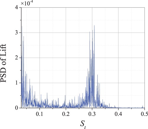In addition, the values of $|{\chi }_{Du}{|}^2$ and $|{\chi }_{Dw}{|}^2$ increase as the reduced frequency increases in the high-reduced frequency range, rather than decreasing as in the Sears function, which was also reported by previous studies (Chen et al., 2009; Diana et al., 2002; Han et al., 2010).

Figure 22. AAFs of the Great Belt East Bridge box girder section. The estimated vortex shedding frequency is indicated by a vertical line (dashed red). (a) $|{\chi }_{Lu}{|}^2$, (b) $|{\chi }_{Du}{|}^2$, (c) $|{\chi }_{Mu}{|}^2$, (d) $|{\chi }_{Lw}{|}^2$, (e) $|{\chi }_{Dw}{|}^2$, (f) $|{\chi }_{Mw}{|}^2$.

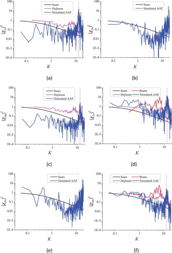
Figure 23. Spectral analysis of the lift time histories of the girder section at zero angle of attack.

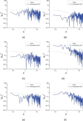
The $\mathrm{\Pi }$ type girder section of the Danjiang Reservoir Bridge is typically bluff body. Both the flow pattern and distribution characteristics of the fluctuating pressures are significantly different from those of thin plate, as well as the corresponding AAFs. Figure 24 shows the computed six AAF components of the $\mathrm{\Pi }$ type girder section, respectively. Except for $|{\chi }_{Mw}{|}^2$, the difference between the other AAF components and the Sears function is apparent in the investigated frequency range. Particularly, the computed $|{\chi }_{Lw}{|}^2$ are much higher than those of the Sears function and the streamlined box girder section. The results shown in Figure 24 prove again that the Sears function fails to predict the AAFs of the bluff bridge girder section, and the AAFs relating to the longitudinal velocity component are different from those corresponding to the vertical velocity component.

Figure 24. AAFs of the Danjiang Reservoir Bridge box girder section: (a) $|{\chi }_{Lu}{|}^2$, (b) $|{\chi }_{Du}{|}^2$, (c) $|{\chi }_{Mu}{|}^2$, (d) $|{\chi }_{Lw}{|}^2$, (e) $|{\chi }_{Dw}{|}^2$, (f) $|{\chi }_{Mw}{|}^2$.

6. Conclusions

In this study, a turbulent wind field is generated as the inflow boundary of the LES based on the DSRFG method. The pattern of the variation in the turbulent wind along the computational domain is investigated under consideration of various grid sizes and time step sizes. The AAFs of a thin plate and two typical bridge girder sections are numerically predicted by LES. The following conclusions are summarized:

1. The DSRFG technique is a reliable method to generate the inflow boundary condition with specified statistical characteristics for LES. Moreover, the DSRFG method is convenient to implement for parallel computing.

2. The turbulence properties are well maintained in the computational domain. The grid size investigated in the present study has little influence on the mean velocity and turbulence intensity. The energy of the simulated spectrum decays in the high-frequency range, and this effect can be improved by applying finer grids and smaller time step sizes. Based on the present study, it is suggested that a grid system with a resolution of 1 cm and a time step size of dt = 1 × 10⁻⁴ s can provide a reasonable turbulent wind field. In addition, if more computational resource is available, the computational domain should be larger than the one employed in the present study in order to eliminate the boundary influences, such as girder length longer than 0.5B in spanwise direction, and increased distance from trailing edge of the model to the outlet boundary.

3. Fairly good agreement between the estimated AAF of a thin plate and the Sears function validate the feasibility of the LES in predicting the AAFs. The flow pattern and pressure distribution of bridge deck sections, especially the $\mathrm{\Pi }$ type girder section, are significantly different from those of the thin plate, and the Sears function fails to predict the AAFs of the bluff bridge girder section. The contributions of the longitudinal and vertical velocity components to the buffeting forces are not equal, and it is inappropriate to employ one equivalent AAF for each force component.

To ensure the prescribed turbulent properties are well maintained along the computational domain, very fine mesh should be set between the inlet boundary and the girder, which leads to considerable computational cost. In the present study, the turbulence intensity slightly decays in the windward direction and the turbulence energy of the wind spectra may decay in the high-frequency range, which may affect the aerodynamic responses. In future work, a more efficient and accurate inflow turbulence generation technique should be proposed based on the existing DSRFG method.

Disclosure statement

No potential conflict of interest was reported by the author(s).

Additional information

Funding

This work was supported by Major State Basic Research Development Program of China (973 Program) under [grant number 2015CB057701]; Natural Science Foundation of China under [grant number 51878269]; and Hunan Provincial Innovation Foundation for Postgraduate under [grant number 521293361].

References

- Aboshosha, H., Elshaer, A., Bitsuamlak, G. T., & El Damatty, A. (2015). Consistent inflow turbulence generator for LES evaluation of wind-induced responses for tall buildings. Journal of Wind Engineering and Industrial Aerodynamics, 142, 198–216. https://doi.org/10.1016/j.jweia.2015.04.004
- Batten, P., Goldberg, U., & Chakravarthy, S. (2004). Interfacing statistical turbulence closures with large-eddy simulation. AIAA Journal, 42(3), 485–492. https://doi.org/10.2514/1.3496
- Bruno, L., Tubino, F., & Solari, G. (2005). Aerodynamic admittance functions of bridge deck sections by CWE. Proc., EURODYN.
- Castro, H. G., & Paz, R. R. (2013). A time and space correlated turbulence synthesis method for large eddy simulations. Journal of Computational Physics, 235, 742–763. https://doi.org/10.1016/j.jcp.2012.10.035
- Chen, B., Ge, Y. J., & Xiang, H. F. (2009). Aerodynamic admittance identification for non-streamline section by method of zero-sparation. Journal of Tongji University (Natural Science), 37(22), 155–158. (in Chinese).
- Chen, X. Y., Wang, B., Zhu, L. D., & Li, Y. L. (2018). Numerical study on surface distributed vortex-induced force on a flat-steel-box girder. Engineering Applications of Computational Fluid Mechanics, 12(1), 41–56. https://doi.org/10.1080/19942060.2017.1337593
- Davenport, A. G. (1962). Buffeting of a suspension bridge by storm winds. Journal of Structural Division, ASCE,, 88(3), 233–268.
- Dhamankar, N. S., Blaisdell, G. A., & Lyrintzis, A. S. (2018). Overview of turbulent inflow boundary conditions for large-eddy simulations. AIAA Journal, 56(4), 1317–1334. https://doi.org/10.2514/1.J055528
- Diana, G., Bruni, S., Cigada, A., & Zappa, E. (2002). Complex aerodynamic admittance function role in buffeting response of a bridge deck. Journal of Wind Engineering and Industrial Aerodynamics, 90(12–15), 2057–2072. https://doi.org/10.1016/S0167-6105(02)00321-5
- Ferziger, J. H., & Peric, M. (2002). Computational methods for fluid dynamics. (3rd ed.) Springer.
- Flay, R. G. J., & Stevenson, D. C. (1988). Integral length scales in strong winds below 20 m. Journal of Wind Engineering and Industrial Aerodynamics, 28(1), 21–30. https://doi.org/10.1016/0167-6105(88)90098-0
- Ghalandari, M., Shamshirband, S., Mosavi, A., & Chau, K.-w. (2019). Flutter speed estimation using presented differential quadrature method formulation. Engineering Applications of Computational Fluid Mechanics, 13(1), 804–810. https://doi.org/10.1080/19942060.2019.1627676
- Gu, M., & Qin, X. R. (2004). Direct identification of flutter derivatives and aerodynamic admittances of bridge decks. Engineering Structures, 26(14), 2161–2172. https://doi.org/10.1016/j.engstruct.2004.07.015
- Han, Y., Chen, Z. Q., & Hua, X. G. (2010). New estimation methodology of six complex aerodynamic admittance functions. Wind and Structures An International Journal, 13(3), 293–307. https://doi.org/10.12989/was.2010.13.3.293
- Hejlesen, M. M., Rasmussen, J. T., Larsen, A., & Walther, J. H. (2015). On estimating the aerodynamic admittance of bridge sections by a mesh-free vortex method. Journal of Wind Engineering and Industrial Aerodynamics, 146, 117–127. https://doi.org/10.1016/j.jweia.2015.08.003
- Hémon, P., & Santi, F. (2007). Simulation of a spatially correlated turbulent velocity field using biorthogonal decomposition. Journal of Wind Engineering and Industrial Aerodynamics, 95(1), 21–29. https://doi.org/10.1016/j.jweia.2006.04.003
- Hoshiya, M. (1972). Simulation of multi-correlated random processes and application to structural vibration problems. Proceedings of the Japan Society of Civil Engineers, 1972(204), 121–128. https://doi.org/10.2208/jscej1969.1972.121
- Huang, S. H., Li, Q. S., & Wu, J. R. (2010). A general inflow turbulence generator for large eddy simulation. Journal of Wind Engineering and Industrial Aerodynamics, 98(10–11), 600–617. https://doi.org/10.1016/j.jweia.2010.06.002
- Kondo, K., Murakami, S., & Mochida, A. (1997). Generation of velocity fluctuations for inflow boundary condition of LES. Journal of Wind Engineering and Industrial Aerodynamics, 67-68, 51–64. https://doi.org/10.1016/S0167-6105(97)00062-7
- Kraichnan, R. H. (1970). Diffusion by a random velocity field. Physics of Fluids, 13(1), 22–31. https://doi.org/10.1063/1.1692799
- Larose, G. L. (1992). The response of a suspension bridge deck to the turbulent wind: The taut-strip model approach. The University of Western Ontario.
- Larose, G. L. (1999). Experimental determination of the aerodynamic admttance of a bridge deck segment. Journal of Fluids and Structures, 13(7–8), 1029–1040. https://doi.org/10.1006/jfls.1999.0244
- Larose, G. L., & Mann, J. (1998). Gust loading on streamlined bridge decks. Journal of Fluids and Structures, 12(5), 511–536. https://doi.org/10.1006/jfls.1998.0161
- Larsen, A. (1993). Aerodynamic aspects of the final design of the 1624 m suspension bridge across the Great Belt. Journal of Wind Engineering and Industrial Aerodynamics, 48(2–3), 261–285. https://doi.org/10.1016/0167-6105(93)90141-A
- Li, J., Tong, L., Wu, J., & Pan, Y. (2019). Numerical investigation of wind influences on photovoltaic arrays mounted on roof. Engineering Applications of Computational Fluid Mechanics, 13(1), 905–922. https://doi.org/10.1080/19942060.2019.1653375
- Li, L. (2007). Study on aerodynamic admittance function of bridge and it's application (Ph.D. Ph.D.). Southwest Jiaotong University.
- Liepmann, H. (1952). On the application of statistical concepts to the buffeting problem. Journal of the Aeronautical Sciences (Institute of the Aeronautical Sciences), 19(12), 793–800. https://doi.org/10.2514/8.2491
- Liu, C., Li, J., Bu, W., Ma, W., Shen, G., & Yuan, Z. (2018). Large eddy simulation for improvement of performance estimation and turbulent flow analysis in a hydrodynamic torque converter. Engineering Applications of Computational Fluid Mechanics, 12(1), 635–651. https://doi.org/10.1080/19942060.2018.1489896
- Ma, C. M., Wang, J. X., Li, Q. S., & Liao, H. L. (2019). 3D aerodynamic admittances of streamlined box bridge decks. Engineering Structures, 179, 321–331. https://doi.org/10.1016/j.engstruct.2018.11.007
- Matsuda, K., Hikami, Y., Fujiwara, T., & Moriyama, A. (1999). Aerodynamic admittance and the `strip theory’ for horizontal buffeting forces on a bridge deck. Journal of Wind Engineering and Industrial Aerodynamics, 83(1–3), 337–346. https://doi.org/10.1016/S0167-6105(99)00083-5
- Mou, B., He, B.-J., Zhao, D.-X., & Chau, K.-w. (2017). Numerical simulation of the effects of building dimensional variation on wind pressure distribution. Engineering Applications of Computational Fluid Mechanics, 11(1), 293–309. https://doi.org/10.1080/19942060.2017.1281845
- Naimul Haque, M., Katsuchi, H., Yamada, H., & Nishio, M. (2014). Investigation of flow fields around rectangular cylinder under turbulent flow by Les. Engineering Applications of Computational Fluid Mechanics, 8(3), 396–406. https://doi.org/10.1080/19942060.2014.11015524
- Patruno, L., & Ricci, M. (2017). On the generation of synthetic divergence-free homogeneous anisotropic turbulence. Computer Methods in Applied Mechanics and Engineering, 315, 396–417. https://doi.org/10.1016/j.cma.2016.11.005
- Rasmussen, J. T., Hejlesen, M. M., Larsen, A., & Walther, J. H. (2010). Discrete vortex method simulations of the aerodynamic admittance in bridge aerodynamics. Journal of Wind Engineering and Industrial Aerodynamics, 98(12), 754–766. https://doi.org/10.1016/j.jweia.2010.06.011
- Salih, S. Q., Aldlemy, M. S., Rasani, M. R., Ariffin, A. K., Ya, T. M. Y. S. T., Al-Ansari, N., Yaseen, Z. M., & Chau, K.-W. (2019). Thin and sharp edges bodies-fluid interaction simulation using cut-cell immersed boundary method. Engineering Applications of Computational Fluid Mechanics, 13(1), 860–877. https://doi.org/10.1080/19942060.2019.1652209
- Sears, W. R. (1941). Some aspects of non-stationary airfoil theory and its practical application. Journal of the Aeronautical Sciences, 8(3), 104–108. https://doi.org/10.2514/8.10655
- Simiu, E., & Scanlan, R. H. (1996). Wind effects on structures—fundamentals and applications to design. John Wiley & Sons, Inc.
- Smirnov, A., Shi, S., & Celik, I. (2001). Random flow generation technique for large eddy simulations and particle-dynamics modeling. Journal of Fluids Engineering-Transactions of the Asme, 123(2), 359–371. https://doi.org/10.1115/1.1369598
- Solari, G., & Piccardo, G. (2001). Probabilistic 3-D turbulence modeling for gust buffeting of structures. Probabilistic Engineering Mechanics, 16(1), 73–86. https://doi.org/10.1016/S0266-8920(00)00010-2
- Tabor, G. R., & Baba-Ahmadi, M. H. (2010). Inlet conditions for large eddy simulation: A review. Computers & Fluids, 39(4), 553–567. https://doi.org/10.1016/j.compfluid.2009.10.007
- Tominaga, Y., Mochida, A., Yoshie, R., Kataoka, H., Nozu, T., Yoshikawa, M., & Shirasawa, T. (2008). AIJ guidelines for practical applications of CFD to pedestrian wind environment around buildings. Journal of Wind Engineering and Industrial Aerodynamics, 96(10–11), 1749–1761. https://doi.org/10.1016/j.jweia.2008.02.058
- Uejima, H., Kuroda, S., & Kobayashi, H. (2008). Estimation of aerodynamic admittance by numerical computation. BBAA VI Interna-tional Colloquium on Bluff Bodies Aerodynamics and Appliea tions, Milano, Italy.
- Zhao, L., & Ge, Y. J. (2015). Cross-spectral recognition method of bridge deck aerodynamic admittance function. Earthquake Engineering and Engineering Vibration, 14(4), 595–609. https://doi.org/10.1007/s11803-015-0048-8
- Zhu, L. D., Zhou, Q., Ding, Q. S., & Xu, Z. R. (2018). Identification and application of six-component aerodynamic admittance functions of a closed-box bridge deck. Journal of Wind Engineering and Industrial Aerodynamics, 172, 268–279. https://doi.org/10.1016/j.jweia.2017.11.002
- Zhu, Z. W., Chen, W., & Yuan, T. (2016). Pressure measurement and aerodynamics investigation on benchmark model of bridge girder for CFD simulations. China Journal of Highway and Transport, 29(11), 49–56. (in Chinese). https://doi.org/10.19721/j.cnki.1001-7372.2016.11.007
- Zhu, Z., Gu, M., & Chen, Z. (2007). Wind tunnel and CFD study on identification of flutter derivatives of a long-span self-anchored suspension bridge. Computer-Aided Civil and Infrastructure Engineering, 22(8), 541–554. https://doi.org/10.1111/j.1467-8667.2007.00509.x