A novel valve-less piezoelectric micropump generating recirculating flow

ABSTRACT

Microfluidic devices or systems to generate recirculating flow are increasingly utilized in the fields of chemistry, biomedicine, biology, with bottlenecks in integration and miniaturization needed a breakthrough. Here, a concept for a highly integrated valve-less piezoelectric micropump generating recirculating flow (VPMGRF) is proposed, simultaneously realizing innovation in theory and method. Based on fluid inertiaand energy dissipation of vortexes, a novel double-loop tube was designed to achieve fluid flow in different directions along various paths, with the flow characteristics at different cross-sectional areas explored through computational fluid dynamics (CFD). Afterwards, as valve bodies, the double-loop tubes were connected with a piezoelectric-actuated chamber to constitute the VPMGRF, which was followed by establishing a theoretical model of the vibration, fluid dynamics, and net flow rate. Eventually, experimental results showed that VPMGRFs could generate internal recirculating flow and had a pump effect. The maximum net flow rate reached 5.19 mL/min at 8 Hz, corresponding to a vibrator amplitude of 35 μm and an output pressure amplitude of 4.27 kPa. Furthermore, the larger the characteristic length of the cross section, the greater the amplitude of the vibrators, the larger the amplitude of output pressure, and the slower the flow rate.

KEYWORDS:

• Micropump
• valve-less piezoelectric pump
• recirculating flow
• CFD

Nomenclature

d	=	Diameter
E	=	Kinetic energy
f	=	Frequency
H	=	Displacement
$\dot{H}$	=	Velocity
$\ddot{H}$	=	Acceleration
K	=	Dimensionless constant
L	=	Distance
l	=	Distance
m	=	Mass
Q	=	Flow rate
R	=	Radius
r	=	Radius
S	=	Sectional area
t	=	Time
u	=	Velocity
Φ	=	Dimensionless parameter
σ	=	Standard deviation
η	=	Conversion efficiency
ΔE	=	Energy losses
ξ	=	Coefficient of energy loss

ρ	=	Density
α	=	Angle
(r, θ)	=	Polar coordinates

Subscript

c	=	Contracting direction
e	=	Expanding direction
i-i	=	Cross section
max	=	Maximum value
min	=	Minimum value

1. Introduction

With the increasing demand for microfluidic technologies and their rapid development, emerging technologies in related fields increase the potential for microfluidic systems to achieve complex functions (Aleman et al., 2019; Jiang et al., 2014; Liao et al., 2018; MacDonald et al., 2003; Mach et al., 2002; Quang et al., 2020; Tsao et al., 2018; Zhu et al., 2019). Theoretical and applied researches on the quantification, diversification, and complexity of flow characteristics in microchannels have advanced, especially in the field of the specific functional flow of microfluidic recirculation. In 2006, Atencia et al. proposed a microfluidic system for separating and extracting particles (Atencia & Beebe, 2006). The system consisted of two closed loops with common microchannels, and the fluid in each loop was driven by a disc pump to realize recirculating flow. Particles of different scales were separated according to the different rotating speed of the discs between pumps. In 2017, Clime et al. proposed a microfluidic system for the isolation and concentration of Phytophthora ramorum (Clime et al., 2017). In their investigation, a spiral loop microchannel was designed, and fluid was driven by a syringe pump to flow along the microchannel. Finally, the pathogens were separated and concentrated based on the inertial lateral migration in curving flows. In the same year, Haber et al. proposed a novel microfluidic platform for real-time polymerase chain reaction (qPCR) (Haber et al., 2017). A closed loop was designed on a microfluidic chip, and then, a valve-less piezoelectric micropump with a conical channel was integrated into the loop to drive the fluid flow along the loop. Finally, the target gene to be detected could be amplified and duplicated in thermal circulation flow to provide sufficient targets for further pathogen detection. In 2018, Wang et al. designed a microphysical system (MPS) for culturing vascular endothelial cells (Y. I. Wang & Shuler, 2018). Two liquid storage cavities were designed on a chip, connected by different microchannels. Then the chip was placed on a rocker plane to make it swing back and forth at a certain angle, resulting in a liquid level difference between the storage cavities. Under the action of the height difference, the liquid circulated in the microchannel. In 2019, Sangjo et al. proposed a chip with recirculating microfluidics to model the communication between a tumor and lymph in vitro (Shim et al., 2019). A rectangular closed-loop microchannel was designed on a dual-slice chip, and the fluid was driven by a micropump to circulate.

As far as existing research is concerned, most utilized an externally separated power system to drive the microfluidics in annular channels, thus achieving recirculating flow. However, these kinds of designs have common obvious shortcomings: (a) From a methodological perspective, the functional modular design makes it difficult to coordinate among modules, which brings about the challenge of accurate control strategy; (b) on a practical level, the assembly and mechanical coordination of modules require high standards for microstructural machining. This is not conducive to miniaturization for a microfluidic device, with huge space and time resources to occupy. Therefore, it is of great significance to construct a highly integrated microfluidic device with multiple functions that can drive microfluidics and generate circulating flow at the same time. On account of this novel conception, a novel microsystem with integrated function is designed to combat the limitations of the traditional concept and achieve innovations in terms of the implementation method. This will accelerate the integration and miniaturization of microfluidic devices and provide a new approach for microfluidic technologies, such as biochemical analysis and biomedicine.

For microfluidic devices, it is vital to select an appropriate driving method. In general, microfluidic driving methods include electrostatic actuation (H. Kim et al., 2015; Teymoori & Abbaspour-Sani, 2005), electromagnetic actuation (Rosenberger, 1930; X.-D. Zhang et al., 2020), shape memory actuation (Saren et al., 2018; Ullakko et al., 2012), and piezoelectric actuation (Bussmann et al., 2021; J. Kan et al., 2008; Wu et al., 2021). Among them, piezoelectric actuation has the characteristics of no electromagnetic interference, high energy density, and low energy consumption. Moreover, the structure and working principle are relatively simple, which makes it easy to miniaturize and integrate. With the above advantages, piezoelectric actuation would be a good choice to integrate into microfluidic devices. In 2013, Zhang et al. proposed a peristaltic piezoelectric micropump for microfluidic systems (W. Zhang & Eitel, 2013). It consisted of three serial microchambers actuated by piezoelectric vibrators that were stimulated at different phases. Finally, a maximum net flow rate of 630mL/min was obtained. In 2015, Lin et al. proposed a printing platform with droplets driven by piezoelectric actuators (Li et al., 2015). The actuators drove the tail of a cantilever rod up and down, forcing a microchannel, thus driving quantified droplets. In 2017, Zhao et al. fabricated a polyvinylidene fluoride (PVDF) piezoelectric membrane as the actuator, which was integrated into a microfluidic chip (Zhao et al., 2017). Then, based on the resistance characteristics of a conical channel, the microfluidics were driven quantitatively and directionally to generate droplets. In 2019, Ma et al. proposed another novel peristaltic micropump for microfluidic chips for which innovation was to fabricate a microchannel that could be deformed (Ma et al., 2019). The piezoelectric actuator exerted a force on the wall of the microchannel to drive the microfluidics, avoiding direct contact and cross-contamination between the conveying fluid and the actuator. Therefore, the piezoelectric driving method will be used in the proposed microfluidic device below.

In this paper, we have been inspired by the cardiovascular circulatory system, where the heart’s pumping drives blood away through the arteries and back through the veins to recirculate the blood. The concept of a highly integrated valve-less piezoelectric micropump generating internal recirculating flow (VPMGRF) is proposed. First, based on inertia of fluid and energy dissipation of vortexes, a novel double-loop flow tube is proposed, which can achieve fluid flow in different directions along various flow paths. Then computational fluid dynamics (CFD) is used to verify the above characteristics. Since it is affected by the inertia of fluid, we investigated the flow characteristics of double-loop flow tubes with different cross section shapes (square or circular) and different cross section areas (square section: characteristic length l = 1.5, 2, or 2.5 mm; circular section: characteristic length d = 1.5, 2, or 2.5 mm). As valve bodies, double-loop tubes were connected with the pump chamber actuated by a piezoelectric vibrator to constitute a micropump. The vibrator forces a periodic change in the volume of the chamber, imitating the pumping of the heart. As a result, fluid is discharged from the chamber to a flow path and then absorbed back along another flow path, so as to realize its recirculation in a loop. Afterwards, a theoretical model of the vibration and fluid dynamics of a double-loop tube was established and the net flow rate of the micropump was analyzed. Eventually, prototypes of double-loop tubes and micropumps were manufactured, and experiments were successfully carried out to verify the flow characteristics of fluid along double-loop tubes. Moreover, the performance of vibrators’ amplitudes, the net flow rate, and the output pressure of micropumps were tested.

2. Double-loop tube and its function of rectification

2.1. Structure of double-loop tube

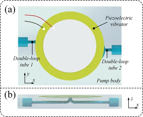
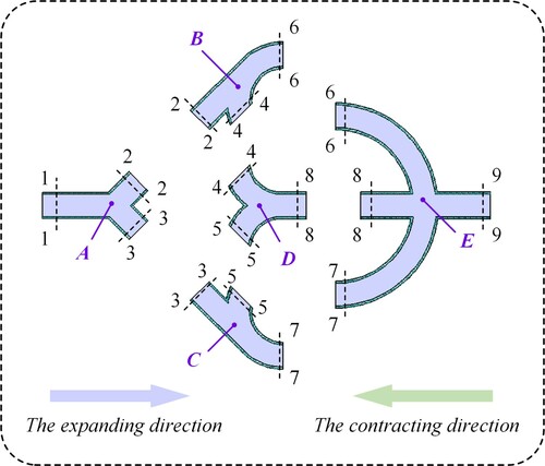
As shown in Figure 1, a double-loop tube is composed of seven parts: Tube j, Tube i₁, Tube i₂, Tube p₁, Tube p₂, Tube q₁, and Tube t. Among them, Tube p₁ and Tube p₂ are semicircular arc tubes, which are symmetrically distributed and combined to form an ε-shaped tube. The middle nozzle of the ε-shaped tube is connected with a straight tube, Tube t, and another two nozzles of the ε-shaped tube are connected by a semicircular arc tube, Tube q. Thus, Tube p₁, Tube p₂, Tube q, and Tube t are combined to form two closed loops with a common channel. In addition, Tube i₁ and Tube i₂, which converge to Tube j at an angle of 2α, are connected with Tube p₁ and Tube p₂, respectively. Finally, Tube j and Tube t are the inlet or outlet. The direction in which fluid flows from Tube j to Tube t is called the expanding direction. On the contrary, the direction the fluid flows from Tube t to Tube j is called the contracting direction. The size parameters of the double-loop tube in Figure 1(b) are shown in Table 1.

Figure 1. Structure of double-loop tube. (a) Three-dimensional structure; (b) Two-dimensional structure; (c) Physical model of double-loop tube.

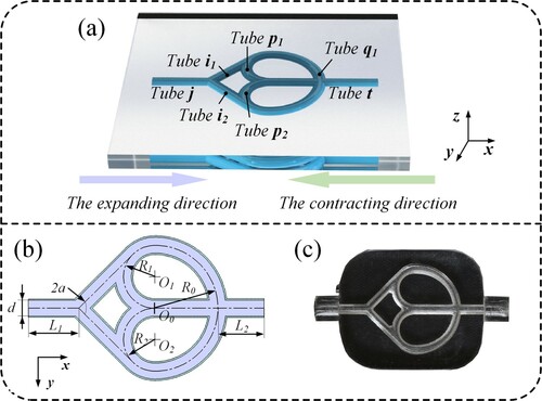
Table 1. Dimensional parameters of double-loop tube.

Parameters	Values
Diameter/d (mm)	2
Distance/L1 (mm)	4
Distance/L2 (mm)	4
Radius/R0 (mm)	8
Radius/R1 (mm)	4
Radius/R2 (mm)	4
Angle/α (°)	90

2.2. Numerical analyses

Computational fluid dynamics (CFD), used to simulate the fluid flow in complex fluid systems, has become a powerful approach for the analysis of engineering problems in various fields. In particular, it is suitable for cases where experimental research is difficult (Ghalandari et al., 2019; Salih et al., 2019). For the present investigation, we use CFD to verify the rectification of the double-loop tube and explore the flow characteristics of tubes at different cross sections.

2.2.1. Rectification of double-loop tube

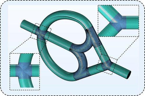
In order to verify the rectification of the double-loop tube, we simulated the fluid flow through it from expanding and contracting directions. First of all, a 3D fluid domain model of a double-loop tube was established, with the parameters presented in Table 1. Next, it was meshed to solve the equations. As is known, the unstructured mesh method has good adaptability to geometric models and is often used to divide complex areas into grids. Using a structured mesh method makes computational convergence easier, saves calculation time, and is suitable to mesh regular geometric models. To get a better quality of mesh, the fluid domain model was divided into several parts and the mixed mesh method was used to mesh the double-loop tube as shown in Figure 2. The bifurcation parts of the double-loop tube were meshed with unstructured grids and the rest of the parts were meshed with structured grids. Then, to further evaluate the grid independency, different degrees of grid size were set to generate grids and the optimal number was selected. Eventually, the total number of elements was 1.8 × 10⁶. Among them, the number of elements used for meshing with unstructured grids was 1.0 × 10⁶ and the number of structured grids was 0.8 × 10⁶.

Figure 2. The finite element model of double-loop tube.

As for boundary conditions, the nozzles of the tube are defined as the inlet or outlet according to the direction of fluid flow. The inlet was set to a pressure of 100 Pa, while the outlet had open boundaries and a relative pressure of 0. For the wall surfaces of the tube, they were regarded as having nonslip boundary conditions. Then water at 25°C was selected as the working medium, with a dynamic viscosity of 8.9 × 10⁻⁴ Pa·s and a density of 997 kg/m³. In addition, fluid in the double-loop tube was driven by the pressure difference between the inlet and outlet, which was regarded as incompressible flow.

To simplify the flow model, unsteady Navier–Stokes equations were used to deal with a steady model invariant over time, based on the Reynolds-averaged Navier–Stokes (RANS) model. Furthermore, due to the complex vortex motions in the bifurcation parts of the double-loop tube, the Realizable K-ε model was selected as the turbulence model, and the steady-state analysis was used. As a result, the simulation of the flow field in different directions was obtained as shown in Figure 3.

Figure 3. Velocity vector on x-y plane of double-loop tube.

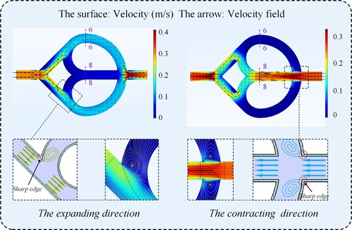
According to the velocity vector marked with the arrows in Figure 3, fluid flows through the side passage of the double-loop tube in the expanding direction. However, it flows through the middle passage in the contracting direction. In different directions, the fluid will flow through different passages, which is called the function of rectification. As for the reason, this phenomenon can be explained by the inertia of fluid and the energy dissipation of vortexes. On the one hand, when fluid flows through the bifurcation sections of a tube, it will mainly flow along the original direction due to the inertia. On the other hand, there are several sharp edges at the bifurcation sections. They will contribute to form Helmholtz discontinuity and generate vortexes, constantly consuming the kinetic energy of the fluid and slowing down the flow in consequence.

From the above simulation results, it can be concluded that a double-loop tube provides the function of rectification. It can achieve fluid flow from different directions along various flow paths, which plays a role in diverting the flow to a specific passage. What is more, fluid inertia is the main factor affecting the rectification effect. Hence, an appropriate increase of fluid velocity may be beneficial to improve the rectification effect.

2.2.2. Influence of double-loop tube’s cross section on rectification

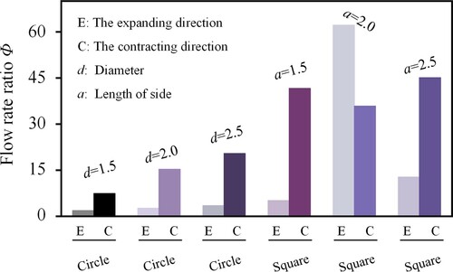
To further explore the relationship between the fluid inertia and the rectification effect, six different sets of double-loop tubes with different cross section shapes and areas were designed. From Section 2.2.1, we know that the rectification of the double-loop tube is mainly based on the inertia of the fluid. So, selecting a smaller characteristic length is beneficial to increase the velocity of the fluid in the tube, which can bring about a better rectification effect. We know that 1.5 mm is the minimum characteristic length of tubes to obtain a better physical model through 3D printing. Therefore, we selected a minimum characteristic length of 1.5 mm and an interval of 0.5 mm. The dimensional parameters are shown in Table 2. Then their flow field was simulated through the same method and setting as above. Simulation results of flow rates through cross sections 6–6 and 8–8 are viewed regarded as the flow rates through the side passage and the middle passage, respectively. We used the dimensionless parameter Φ to represent the ratio of the flow rate through cross sections 6–6 and 8–8 during the expanding or contracting process: (1) ${\mathrm{\Phi }}_x=\frac{f_{\text{max}}\left\{{\left(Q_{6-6}\right)}_x,{\left(Q_{8-8}\right)}_x\right\}}{f_{\text{min}}\left\{{\left(Q_{6-6}\right)}_x,{\left(Q_{8-8}\right)}_x\right\}},$(1) where $(Q_{6-6}{)}_x$ and $(Q_{8-8}{)}_x$ are the flow rate through cross sections 6–6 and 8-8, respectively, obtained from the expanding or contracting process. The subscript x represents the direction of the fluid flow. When x is c, it indicates that the fluid flows in the contracting direction; when x is e, the fluid flows in the expanding direction. f_max and f_min are the maximum and minimum between $(Q_{6-6}{)}_x$ and $(Q_{8-8}{)}_x$, respectively. It should be noted that $(Q_{6-6}{)}_x$ and $(Q_{8-8}{)}_x$ in Equation (1) are obtained from the same direction of fluid movement.

Table 2. Dimensional parameters of double-loop tubes.

Category	Cross-section shape of tubes	Sectional dimension
Tube A	Circle	φ1.5mm
Tube B	Circle	φ2.0mm
Tube C	Circle	φ2.5mm
Tube D	Square	1.5×1.5mm
Tube E	Square	2.0×2.0mm
Tube F	Square	2.5×2.5mm

In addition, when ${\mathrm{\Phi }}_x$ is larger, it indicates that the fluid is more inclined to flow along a certain flow path. This is the function of the rectification mentioned in Section 2.2.1. Therefore, the dimensionless parameter ${\mathrm{\Phi }}_x$ can also reflect the effect of rectification.

The results of rectification between different groups of double-loop tubes are shown in Figure 4. For double-loop tubes with a circular cross section, the rectification of fluid in both directions became more obvious as the diameter of the tube increased. Moreover, it was more obvious in the expanding direction than in the contracting direction. For the square cross section, the double-loop tubes with a characteristic length of l = 2.0 mm had the most obvious rectification when the fluid flowed in the expanding direction. The flow characteristics among different lengths is almost consistent when the fluid flows in the contracting direction. In addition, by comparing the flow characteristics of different double-loop tubes, it can be concluded that the rectification effect of double-loop tubes with a square cross section is much better. Among the six different sets of double-loop tubes, Tube E, for which the cross section is square with a characteristic length of l=2.0 mm, has the best performance of rectification.

Figure 4. Results of rectification between different groups of double-loop tubes.

As there are machining size errors in the actual manufacturing process of the tubes, it is necessary to analyze the stability of the rectification effect when the characteristic length of the cross section changes. Then, the standard deviation $\sigma$ is used to represent the stability: (2) ${\sigma }^2=\frac{1}{N}\sum _{i=1}^N({\mathrm{\Phi }}_{xi}-\overline{{\mathrm{\Phi }}_x}{)}^2,$(2) where ${\mathrm{\Phi }}_{xi}$ is the flow rate ratio, x_i represents the characteristic length, and $\overline{{\mathrm{\Phi }}_x}$ is the average value of ${\mathrm{\Phi }}_{xi}$.

Thus, the rectification effects of fluid in a different direction can be obtained as shown in Tables 3 and 4.

Table 3. Rectification effect of fluid in the expanding direction.

Ratio Φe	x1=1.5	x2=2.0	x3=2.5	Average value $\overline{{\mathrm{\Phi }}_e}$	Standard deviation ${\sigma }_e$
Circle (y1)	1.88	2.68	3.49	2.68	0.66
Square (y2)	5.17	62.15	12.79	26.70	25.26

Table 4. Rectification effect of fluid in the contracting direction.

Ratio Φc		x1=1.5	x2=2.0	x3=2.5	Average value $\overline{{\mathrm{\Phi }}_c}$	Standard deviation ${\sigma }_c$
y1	Circle	7.43	15.32	20.44	14.40	5.35
y2	Square	41.64	35.83	45.11	40.86	3.83

The following relationship can be obtained from the data above: (3) $\begin{array}{rl}{\sigma }_e\left(y_1\right)& \ll {\sigma }_e\left(y_2\right)\end{array}$(3) (4) $\begin{array}{rl}{\sigma }_c\left(y_1\right)& \approx {\sigma }_e\left(y_2\right).\end{array}$(4)

From Equation (3), we know that the change in the square cross section size has a greater influence on the rectification effect in the expanding direction, compared with that of a circular cross section. However, the influence of the cross-sectional area on the rectification effect in the contracting direction is similar between the circular cross section and the square section according to Equation (4). Therefore, it can be concluded that a change in the cross-sectional area has a greater influence on the stability of rectification for square cross section double-loop tubes.

3. VPMGRF and its recirculating flow

Piezoelectric pumps are composed of a piezoelectric actuator and valve body (Chen et al., 2020; Kaynak et al., 2016; Li et al., 2021; J. T. Mohith et al., 2019; Opekar et al., 2016; Tang et al., 2019; Valdovinos et al., 2014; Wang et al., 2019; Y.-N. Wang & Fu, 2018; Yin et al., 2020). The actuator provides power for the fluid and the valve body plays a diversion role, so as to achieve unidirectional fluid pumping. In general, valve bodies can be classified into those with moving parts (Bao et al., 2019; Carrozza et al., 1995; Dong et al., 2017; Feng & Kim, 2004; L. He et al., 2020; J. W. Kan et al., 2005; Nguyen & Truong, 2004; Zeng et al., 2016) and those with nonmoving parts. Furthermore, nonmoving parts include conical tubes (He et al., 2017; Tseng et al., 2013), Y-shaped tubes (Huang et al., 2013, 2016), heterotypic tubes (Izzo et al., 2007), spiral tubes (Leng et al., 2013), vortex diodes (Huang et al., 2019), unsymmetrical chambers with blocks arranged (Xia et al., 2012), etc. The nonmoving parts are based on the flow resistance mechanism to realize unidirectional fluid pumping macroscopically.

With the function of rectification, double-loop tubes can be regarded as valve bodies with nonmoving parts. They were connected to the pump chamber actuated by the piezoelectric vibrator, thus constituting a valve-less piezoelectric micropump generating recirculation flow (VPMGRF).

3.1. The structure of VPMGRF

As shown in Figure 5, VPMGRF is composed of a piezoelectric vibrator and a pump body. The pump body includes a pump chamber and double-loop tubes. The upper surface of the pump chamber is covered by a piezoelectric vibrator. As the vibrator deforms, a volume change will occur in the pump chamber. In addition, the bottom surface is provided with two chamber outlets that are connected with the double-loop tubes through a bent tube. The diameter of the pump chamber is 27 mm and the depth of pump chamber is 0.8 mm. Moreover, the distance between the chamber outlet and the chamber center is 2 mm, and the radius of the bent tubes is 2.5 mm.

Figure 5. Structure of VPMGRF. (a) Vertical view of VPMGRF; (b) Front view of VPMGRF.

3.2. Working principle of VPMGRF and its recirculating flow

The piezoelectric vibrator is made of a metal plate and a ceramic disc. The direction of polarization of the ceramic disc is along the length. With the surroundings restrained, the vibrator will arch up or press down when applied with excitation. As shown in Figure 6(a), during the suction process, the vibrator is moving upwards, the pump chamber is expanding, and the external fluid is inhaled through double-loop tubes. As shown in Figure 6(b), during the discharge process, the vibrator is moving downwards, the pump chamber is compressed, and the fluid is pressed out from the pump chamber. The suction and discharge processes will form a pumping cycle.

Figure 6. Working principle of VPMGRF. (a) Flow mechanism during suction; (b) Flow mechanism during discharge; (c) Recirculating flow during a pumping cycle.

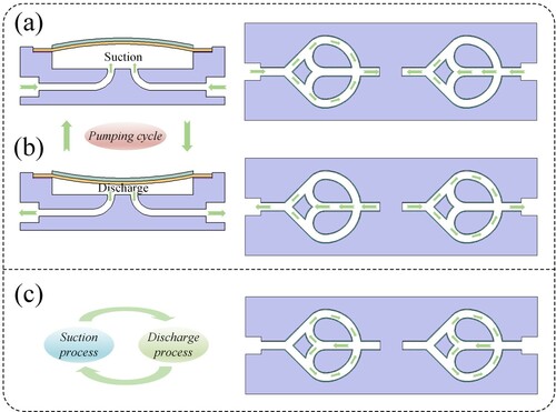
As shown in Figure 6(a, b), due to the rectification of the double-loop tube, fluid flows along different paths during the suction and discharge processes. Therefore, the flow paths of the fluid will reverse during the pumping cycle. To be specific, the fluid passing through the middle passage during the suction process will flow through the side passage during the discharge process. The fluid passing through the side passage during the suction process will flow through the middle passage during the discharge process. As a result, during a pumping cycle, VPMGRF will generate recirculating flow in the partial passage of the double-loop tube, as shown in Figure 6(c).

4. Theoretical model

For power components, a piezoelectric vibrator will vibrate in a first-order mode when applied with low-frequency excitation. The vibrator arches up in the center and the surface of deformation can be considered a paraboloid. Accordingly, the motion of any point over the vibrator can be obtained: (5) $\begin{array}{rl}H& =H\left(r,\theta \right)\text{sin}2\pi ft\end{array}$(5) (6) $\begin{array}{rl}\dot{H}& =\frac{dH}{dt}\end{array}$(6) (7) $\begin{array}{rl}\ddot{H}& =\frac{d\dot{H}}{dt},\end{array}$(7) where $H$, $\dot{H}$, and $\ddot{H}$ are the displacement, velocity, and acceleration of any point on the vibrator; $H\left(r,\theta \right)$ is the maximum amplitude of a location on the vibrator; $f$ is the frequency of the excitation source; and $t$ is the time.

Hence, the kinetic energy generated by the vibrator can be expressed as follows: (8) $\begin{array}{rl}E& =m{\int }_0^{2\pi }d\theta {\int }_0^R\frac{\mathrm{\partial }E\left(r,\theta \right)}{\mathrm{\partial }m}rdr\end{array}$(8) (9) $\begin{array}{rl}\frac{\mathrm{\partial }E\left(r,\theta \right)}{\mathrm{\partial }m}& =\frac{1}{2}(\dot{H}{)}^2,\end{array}$(9) where $E$ and $E\left(r,\theta \right)$ are the total kinetic energy and average kinetic energy per unit mass at a point above the vibrator, and $m$ is the mass of the vibrator.

During the pumping process, the kinetic energy of the vibrator will translate into the kinetic energy of the fluid due to the fluid–structure interaction. Consequently, there is the following relationship: (10) $\begin{array}{r}{E}_0=E\eta ,\end{array}$(10) where $E_0$ is the kinetic energy of the fluid and $\eta$ is the energy conversion efficiency in the case of fluid–structure interaction.

Due to the internal friction of the fluid, there will be energy loss as the fluid flows through double-loop tubes. There will be different energy losses when it flows through double-loop tubes in a different direction. (11) $\begin{array}{rl}\mathrm{\Delta }{E}_c& =E_0{\xi }_c\end{array}$(11) (12) $\begin{array}{rl}\mathrm{\Delta }{E}_e& =E_0{\xi }_e,\end{array}$(12) where $\mathrm{\Delta }{E}_c$ and $\mathrm{\Delta }{E}_e$ are the energy losses in the contracting and expanding directions, respectively, and ${\xi }_c$ and ${\xi }_e$ are the coefficients of energy loss in the contracting and expanding direction, respectively. It should be noted that ${\xi }_c\ne {\xi }_e$. The specific derivation process is given in Appendix A.

Therefore, the energy loss difference drives the fluid pumping in a single direction during the pumping cycle. Accordingly, the net flow rate can be calculated: (13) $\begin{array}{rl}\mathrm{\Delta }E& =|\mathrm{\Delta }{E}_c-\mathrm{\Delta }{E}_e|\end{array}$(13) (14) $\begin{array}{rl}\mathrm{\Delta }E& =\frac{1}{2}\rho v^2\end{array}$(14) (15) $\begin{array}{rl}\text{Q}& =Sv\end{array}$(15) (16) $\begin{array}{rl}\text{S}& =\pi r^2,\end{array}$(16) where $\mathrm{\Delta }E$ is the energy loss difference; $\rho$ is the density of the fluid; $\text{Q}$ is the net flow rate; $S$ is the sectional area of the tube; and $r$ is the radius of tube.

By combining Equations (13)–(16), the following conclusions can be drawn: (17) $\begin{array}{r}\text{Q}=\sqrt{2}\pi r^2{\rho }^{(-1/2)}(E\eta {)}^{\left(1/2\right)}|{\xi }_c-{\xi }_e{|}^{\left(1/2\right)}.\end{array}$(17)

5. Experiments

5.1. Fabrication of VPMGRF

The pump bodies were made of transparent photosensitive resin by SLA (Stereo lithography Apparatus), as shown in Figure 7. The modeling dimensional accuracy is about ±0.1 mm. Then the piezoelectric vibrator was fixed to the pump body using an epoxy resin adhesive. The structural parameters of the vibrator are shown in Table 5. Eventually, prototypes of VPMGRFs were manufactured successfully; their parameters are given in Table 6.

Figure 7. Physical drawing of six sets of sample pumps.

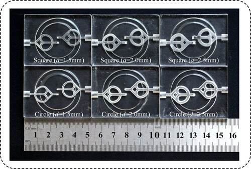
Table 5. Structural parameters of piezoelectric vibrator.

Parameters	Values
Resonant frequency (kHz)	$2.6\pm 0.5\text{kHz}$
Resonant impedance ($\mathrm{\Omega }$)	$<250$
Free capacitance (pF)	$350000\pm 30\mathrm{\%}$
Plate material	Brass
plate diameter (mm)	$35\pm 0.1$
plate thickness (mm)	$0.18\pm 0.02$
plate density (kg/m^3)	$8.5\times {10}^3$
Ceramic disc diameter (mm)	$23\pm 0.2$
Ceramic disc thickness (mm)	0.30
Ceramic disc density (kg/m^3)	$7.5\times {10}^3$
Total weight (g)	1.16g

Table 6. Dimensional parameters of VPMGRF.

Category	Type of double-loop tubes	Cross-section shape	Sectional dimension
Pump A	Tube A	Circle	φ1.5 mm
Pump B	Tube B	Circle	φ2.0 mm
Pump C	Tube C	Circle	φ2.5 mm
Pump D	Tube D	Square	1.5×1.5 mm
Pump E	Tube E	Square	2.0×2.0 mm
Pump F	Tube F	Square	2.5×2.5 mm

5.2. Experimental design

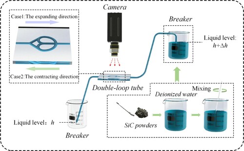
5.2.1. Observation of double-loop tube’s flow characteristics

In order to prove the double-loop tubes’ function of rectification, an experiment was carried out as shown in Figure 8. First, 5 g of silicon carbide powder (with a diameter of 1 μm and a density of 3.20 g/cmm⁻³) were added to 1 L of deionized water in a beaker. Then a glass rod was used to stir them in one direction to suspend them in water. Later, a silicone tube connected to the inlet of the double-loop tube was inserted into the beaker with a suspension liquid. Another silicone tube connected to the outlet was inserted into the empty beaker. To verify the rectification of the double-loop tube, we had to provide a driving power for the fluid to flow through the double-loop tube. Therefore, two beakers were placed at a certain height difference and the liquid could be driven through the double-loop tube by the liquid level difference of Δh. According to the analysis in Section 2.2, the greater the inertia of fluid, the more obvious rectification will be achieved. Therefore, the dimensionless parameter ${\mathrm{\Phi }}_x$ in Equation (1(1) ${\mathrm{\Phi }}_x=\frac{f_{\text{max}}\left\{{\left(Q_{6-6}\right)}_x,{\left(Q_{8-8}\right)}_x\right\}}{f_{\text{min}}\left\{{\left(Q_{6-6}\right)}_x,{\left(Q_{8-8}\right)}_x\right\}},$(1) ) will be influenced by the liquid level difference of Δh. To make sure that the flows in different directions have the same initial velocity, the liquid level difference was set to 10 cm. After that, the positions of the two beakers were interchanged so as to change the direction of flow through the double-loop tube. Finally, the flow fields of fluid in different directions were observed and the flow characteristics of the double-loop tube were obtained.

Figure 8. Experiment schematic of double-loop tube.

5.2.2. Measurement of VPMGRFs’ output performance

The double-loop tubes were connected with a chamber actuated by a piezoelectric vibrator, which constitutes the VPMGRF. The vibrators can provide kinetic energy for a fluid, so an extra height difference between inlet and outlet was not needed. In order to eliminate the influence of the height difference on the output performance of VPMGRFs, performance tests were carried out under the initial conditions of zero back pressure.

As shown in Figure 9, the function signal generator (AFG1022, Tektronix, Beaverton, WA, USA) provided a sinusoidal signal, which was amplified by a power amplifier (HAS4051, NF, Yokohama, Japan) and applied to the piezoelectric vibrator. Meanwhile, an oscilloscope (DSO-X2004A, Keysight, Santa Rosa, CA, USA) was used to monitor the actual working voltage, current, and frequency of the piezoelectric vibrator. Before power excitation was applied to the vibrator, the inlet of VPMGRF was connected to a silicone tube in the beaker full of deionized water. Then the outlet was connected to another beaker over a precision balance to measure the net flow rate under zero back pressure. It was measured at 20, 40, and 60 s. We took the average as the net flow rate and calculated the error bar. Moreover, the outlet was also connected to a dynamic pressure sensor (HM90, HELM, Hamburg, Germany) through a T-junction and the output pressures were measured three times. Afterwards, under the excitation voltage of 100 V RMS (effective voltage), the performances of six pumps were tested. We also explored the effects of voltage and frequency on output performances. Since it is easy to break down piezoelectric ceramics and cause crack damage by using higher exciting voltage, the driving voltage was in the range of 200–300 V (peak-to-peak value).

Figure 9. Experimental setup for performance tests of VPPGRF.

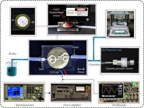
At the same time, we used a laser displacement sensor (LK-H020, Keyence, Osaka, Japan) to measure the vibration of the vibrator. First, we marked nine equally spaced points on the upper surface of the vibrator as shown in Figure 9. Then the movement of these points were measured one by one. Finally, the deformation of the whole vibrator could be obtained by the movement data of these nine points.

5.2.3. Observation of flow field in VPMGRF

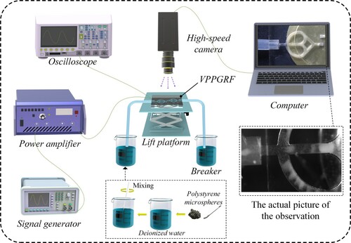
After obtaining the output performance of VPMGRF, we had to further verify the ability to generate recirculating flow. Similarly, the observation of flow field in VPMGRF was carried out under the initial condition of zero back pressure.

As shown in Figure 10, the flow trajectory of the fluid in a double-loop tube during a pumping cycle was observed. First, 5 g of polystyrene microspheres (density: 1.06 g/cmm³; diameter: 10 μm) were added to a beaker with deionized water and a glass rod was used to stir in one direction to mix them well. Then the produced fluid, mixed with microspheres, was used as a working medium during the pumping process. Afterwards, the piezoelectric vibrator was applied with the same voltage excitation as before. Finally, the motion trajectory of the microsphere at this time was captured by a high-speed camera and directly reflected the flow field.

Figure 10. Experimental setup for the flow field during a pumping cycle.

6. Results and discussion

6.1. Flow characteristics of double-loop tubes

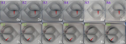
Figure 11 shows the results of flow characteristics when the fluid flowed through the double-loop tube in different directions. As shown in Figures A1–A6, the fluid flowed through the side passage of the double-loop tube in the expanding direction because the silicon carbide powders (marked with arrows) in the middle passage were barely moving. The flow in the contracting direction is shown in Figures B1–B6. The silicon carbide powders (marked with the arrows) in the side passage increased as the flow time went on, which indirectly proves that the fluid in the contracting direction flowed through the middle passage. In addition, there was the center of the vortex (marked with a circle), which is consistent with what was explained in Section 2.2.1.

Figure 11. Result of the flow characteristics when fluid flow through double-loop tube (As shown in video 1 in the attachment).

6.2. Observation of flow field in VPMGRF

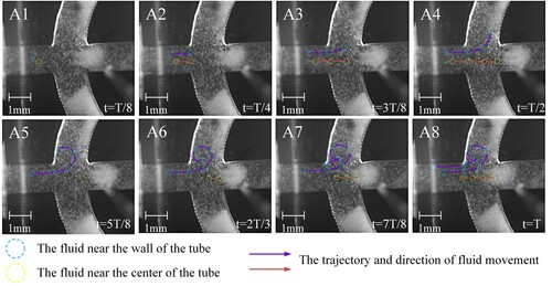
Figure 12 shows the results of observation of the flow field in VPMGRF. Figures A1–A8 represent the actual movement of fluid in a pumping cycle. The circles marked in A1 represent the initial position of the microsphere and the circles in different colors represent the microspheres at different locations in the tube. As the pumping goes on, the movement trajectory and direction of microspheres are shown by the curves with arrows. Fluid near the wall of the tube would rotate when it flowed through the sharp edge of the tube at bifurcation sections. This phenomenon is due to the formation of Helmholtz discontinuity and vortexes, which verifies the theoretical analysis in Section 2.2. Moreover, we can conclude that fluid in the side passage flowed towards the expanding direction macroscopically. As for the fluid near the center of the tube, it flowed towards the contracting direction on the macro level. Therefore, during the pumping process, the fluid would recirculate in the loop of double-loop tubes.

Figure 12. Result of flow flied in VPMGRF during the pumping cycle (As shown in video 2 in the attachment).

6.3. Output performance of VPMGRFs

The deformed surface area of the vibrator can be obtained by measuring the amplitudes of nine points over the vibrator. Figure 13 is the amplitude measuring result on the surface of the vibrator. The amplitude was greatest near the center of the vibrator and decreased gradually along the radial direction. Therefore, the vibrator appeared to arch up and the deformed surface was near a rotating paraboloid.

Figure 13. Result of the amplitude measurement on the surface of vibrator.

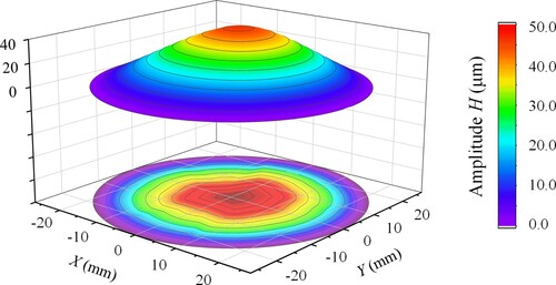
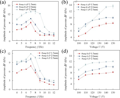
Figure 14 is the amplitude measuring result on the center of the vibrator’s surface between different pumps with different double-loop tubes. Figure 14(a, c) gives the results of amplitude, which varied with frequency under a fixed alternating voltage of 100 V RMS (effective voltage). Moreover, Figure 14(b, d) are the measurement results, which varied with voltage under a fixed frequency corresponding to the maximum flow rate. The voltage was in the range of 100–150 V (peak value).

Figure 14. Amplitude measuring results of different pumps: (a) Amplitude of vibrator over pumps with different circle cross-section tubes under a fixed voltage; (b) Amplitude of vibrator over pumps with different circle cross-section tubes under a fixed frequency; (c) Amplitude of vibrator over pumps with different square cross-section tubes under a fixed voltage; and (d) Amplitude of vibrator over pumps with different square cross-section tubes under a fixed frequency.

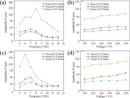
As for the pumps with circle cross section tubes, Pump A (d = 1.5 mm) and Pump B (d = 2.0 mm) had maximum amplitudes of 41 and 52 μm, respectively, at 7 Hz. Pump C (d = 2.5 mm) had a maximum value of 145 μm at 8 Hz. As for the pumps with square cross section tubes, Pump D (l = 1.5 mm) and Pump E (l = 2.0 mm) had maximum amplitudes of 37 and 59 μm, respectively, at 7 Hz. Pump F (l = 2.5 mm) had a maximum value of 165 μm at 6 Hz. From the measurement results of these six pumps, it can be concluded that the amplitude increased as the characteristic length of the cross section increased. In spite of this, there were some things in common between them. On the one hand, the amplitude curves varied and the vibrator frequency curves approximated a parabola that first increases and then decreases. On the other hand, the amplitude of the vibrator increased slowly in a certain voltage range.

Figure 15 shows the results of net flow rate over time. Before applying power excitation, the liquid level of the two beakers was the same and both of them held deionized water with a dye that does not spread easily. The right beaker had red dye added to it, while the left had black dye added. When AC excitation was applied to the vibrator, the liquid in the right beaker began to flow along the silicone tube towards the left beaker and the reading on the precision balance gradually increased. However, when the vibrator was powered off after 60 s, the liquid in the left beaker began to flow back to the right on account of the liquid level differential pressure. The above phenomenon indicates that VPMGRF can overcome the reflux and drive the fluid flow towards the left. According to the continuity of fluid, the increasing reading on the precision balance proved that the pump directed the fluid on the right to the left. Hence, it had the function of pumping the fluid in a single direction, along the expanding direction.

Figure 15. Measurement of net flow rate over time. (As shown in video 3 in the attachment).

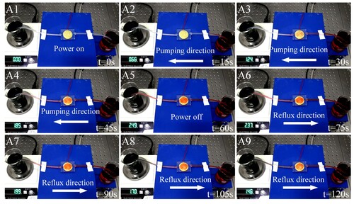
Figure 16 shows the results of net flow rate between pumps. Pump A (d = 1.5 mm) and Pump B (d = 2.0 mm) had the maximum net flow rate of 5.19 and 4.77 mL/min, respectively, at 8 Hz. Pump C (d = 2.5 mm) had the maximum value of 4.01 mL/min at 9 Hz. Pump D (l = 1.5 mm), Pump E (l = 2.0 mm), and Pump F (l = 2.5 mm) had maximum net flow rates of 3.04, 3.31, and 1.36 mL/min, respectively, at 7 Hz. By comparing the pumps with different cross section shapes of double-loop tubes, it can be concluded that the pumps with circular cross section double-loop tubes performed better in terms of the flow rate. Comparing the pumps with different cross section characteristic length of double-loop tubes, we saw that the larger the section length, the smaller the net flow rate. In addition, the trends of net flow rate curves were similar to those of amplitude curves in Figure 14.

Figure 16. Net flow rate measuring result of different pumps. (a) Net flow rate of pumps with different circle cross-section tubes under a fixed voltage; (b) Net flow rate of pumps with different circle cross-section tubes under a fixed frequency; (c) Net flow rate of pumps with different square cross-section tubes under a fixed voltage; (d) Net flow rate of pumps with different square cross-section tubes under a fixed frequency.

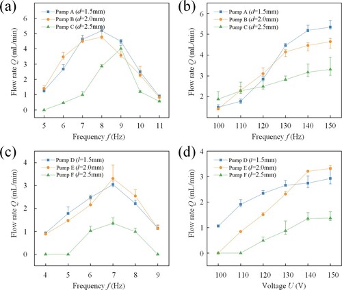
Figure 17 shows the instantaneous output pressure of pumps over time. The initial waveform was a sinusoidal waveform with ‘noise’ but became a smooth waveform curve after 0.05 Hz FFT (Fast Fourier Transformation) lowpass filtering. Then the difference between the maximum and minimum output pressure was defined as the pulsating pressure amplitude, represented by ΔP. Thus, the variation in pressure amplitude with respect to frequency and voltage could be obtained as shown in Figure 18. Pumps A–F had a maximum amplitude pressure of 8.23, 10.08, 13.28, 7.85, 10.19, and 11.88 kPa, respectively, at 7 Hz. For these pumps with different section shapes and characteristic lengths, the performance curves of pressure amplitude showed good consistency. It was obvious that the larger the characteristic length, the greater the amplitude of pressure.

Figure 17. Relationship between the instantaneous output pressure of pumps and time.

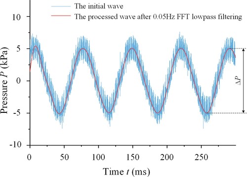
Figure 18. Measuring result of the output pressure amplitude: (a) Output pressure amplitude of pumps with different circle cross-section tubes under a fixed voltage; (b) Output pressure amplitude of pumps with different circle cross-section tubes under the a fixed frequency; (c) Output pressure amplitude of pumps with different square cross-section tube under a fixed voltage; (d) Output pressure amplitude of pumps with different square cross-section tubes under a fixed frequency.

6.4. Discussion of performance difference between the pumps

By comparing the group of curves in Figure 14, Figures 16 and 18, we can draw the following conclusions. For the pumps with the same cross section shaped tubes, the larger the characteristic length of the cross section, the greater the amplitude of the vibrators and output pressure amplitude, while the flow rate decreases. This is because the fluid resistance is related to the cross-sectional area of the tube. As the cross-sectional area increases, the fluid is subjected to less resistance and it causes lower energy loss. Therefore, the vibrator is subjected to a smaller reaction force from the fluid and the amplitude becomes greater. As for the flow rate, the unidirectional pumping of a fluid is realized by the difference in flow resistance. With an increase in the cross-sectional area, the flow resistance decreases and the flow resistance difference narrows; hence, the net flow rate will decrease. In addition, it can also be explained from the perspective of energy consumption. The output power of a pump can be expressed as the product of flow rate and output pressure. When the excitation source applied to vibrator is constant, the greater the output pressure, the smaller the flow rate.

In addition, there was a slight difference in the excitation frequency corresponding to the maximum amplitude of vibrator, net flow rate, and amplitude of output pressure. This is because they are produced in a certain sequence, rather than at the same time. To be specific, the piezoelectric vibrator first acts on the fluid, then the fluid is subjected to resistance to produce pressure, and lastly the flow rate is generated due to the difference resistance. In the transfer process of the three physical quantities, there are some transfer functions, such as pure time delay element, integration loop, differentiation loop, etc., which make the phase-frequency characteristics change. In addition, during the experiment, mechanical fatigue may occur due to the constant vibration of the vibrator, which changes the stiffness of structure and results in the offset of the resonance point. However, on the whole, the frequency corresponding to the maximum amplitude of vibrator, net flow rate, and amplitude of output pressure was approximately in agreement.

7. Conclusions

In this paper, the concept of a highly integrated valve-less piezoelectric micropump generating internal recirculating flow (VPMGRF) was proposed. First, based on the inertia of fluid and the energy dissipation of vortexes, a novel double-loop flow tube was proposed to achieve fluid flow in different directions along various flow paths. Then, the flow field in a double-loop tube was simulated and the flow characteristics of double-loop tubes with different cross section shapes and areas were investigated. After that, the double-loop tubes were connected with a pump chamber to realize the recirculation of fluid in the loop. The theoretical model of vibration, the fluid dynamics, and the net flow rate were established. Eventually, experiments were designed to successfully prove the flow characteristics of the double-loop tubes, and the output performances of micropumps were tested. The following results were obtained:

• The novel double-loop flow tube had the function of rectification. Different cross section shapes and characteristic lengths had an influence on its rectification. Among the six kinds of tubes, the double-loop tube with the square cross section and a characteristic length of l = 2.0 mm had the best rectification performance.

• VPMGRF could generate an internal recirculating flow and had a unidirectional pumping effect on the macro level. Its net flow rate could reach a maximum value of 5.19 mL/min.

• The cross section shapes and characteristic lengths affect the output performances of VPMGRFs. The larger the characteristic length of the cross section, the greater the amplitudes of the vibrator and the output pressure, while the flow rate would decrease.

A valve-less piezoelectric micropump generating recirculating flow (VPMGRF) was proposed for the first time and the performance was successfully verified in this paper. However, there are still many problems that deserve further investigation. As to the VPMGRF itself, the effects of other geometrical parameters on output performances are unknown, such as the angle α between the bifurcated tubes, the radius R₀, R₁, and R₂ of the curvature of arc tubes, etc. Moreover, the diameters of the double-loop tubes in current research are on the millimeter scale. Since MEMS micromachining technologies have appeared, such as deep reactive ion etching and electron beam lithography, it has become easy to achieve the miniaturization of microfluidic devices. The performance of VPMGRFs within the micro–nano scale must be explored, which will accelerate their application in the fields of chemistry, biomedicine, and biology.

Acknowledgements

The authors would like to thank the Guangdong Basic and Applied Basic Research Foundation (grant number 2019B1515120017) and the Natural science foundation of Guangdong (grant number 2018A030310311) for the financial support.

Disclosure statement

No potential conflict of interest was reported by the author(s).

Additional information

Funding

This work was supported by the Guangdong Basic and Applied Basic Research Foundation [grant number 2019B1515120017] and the Natural Science Foundation of Guangdong [grant number 2018A030310311].

A

As shown in Figure A1, the double-loop tube can be divided into five parts, namely Part A, Part B, Part C, Part D, and Part E. According to the method of nodal analysis, the energy losses of fluid flowing through each part are analyzed. At the bifurcation of each part, the cross-sectional area of the tube will mutate. This will intensify the shear stress in the fluid layer, which results in obvious energy loss. The local energy loss coefficient can be expressed by a matrix as follows: (A1) $\begin{array}{r}\left(\begin{array}{cc}{\xi }_i& {{\xi }_i}^{\mathrm{\prime }}\end{array}\right)=\left(\begin{array}{cc}{\xi }_1& {{\xi }_1}^{\mathrm{\prime }}\\ {\xi }_2& {{\xi }_2}^{\mathrm{\prime }}\\ \begin{array}{c}{\xi }_3\\ \begin{array}{c}{\xi }_4\\ {\xi }_5\end{array}\end{array}& \begin{array}{c}{{\xi }_3}^{\mathrm{\prime }}\\ \begin{array}{c}{{\xi }_4}^{\mathrm{\prime }}\\ {{\xi }_5}^{\mathrm{\prime }}\end{array}\end{array}\end{array}\right),\end{array}$(A1) where ${\xi }_i$ and ${{\xi }_i}^{\mathrm{\prime }}$ are the energy loss coefficients in Part i in the expanding direction and in the contracting direction, respectively. ${\xi }_1$–${\xi }_5$ correspond to Parts A– E, respectively.

When fluid flows through a tube with a constant cross section, the energy loss is mainly due to the shear stress between the fluid layers. Generally, it is not on the same order of magnitude as the energy loss at the bifurcation and, thus, can be ignored. Accordingly, the energy loss of fluid at each part is as follows: (A2) $\begin{array}{rl}& \left(\begin{array}{cc}\mathrm{\Delta }{E}_i& {\mathrm{\Delta }{E}_i}^{\mathrm{\prime }}\end{array}\right)\\ & =\left(\begin{array}{cc}\mathrm{\Delta }{E}_1& \mathrm{\Delta }{E_1}^{\mathrm{\prime }}\\ \mathrm{\Delta }{E}_2& \mathrm{\Delta }{E_2}^{\mathrm{\prime }}\\ \begin{array}{c}\mathrm{\Delta }{E}_3\\ \begin{array}{c}\mathrm{\Delta }{E}_4\\ \mathrm{\Delta }{E}_5\end{array}\end{array}& \begin{array}{c}\mathrm{\Delta }{E_3}^{\mathrm{\prime }}\\ \begin{array}{c}\mathrm{\Delta }{E_4}^{\mathrm{\prime }}\\ \mathrm{\Delta }{E_5}^{\mathrm{\prime }}\end{array}\end{array}\end{array}\right)\\ & =\frac{1}{2}\rho \left(\begin{array}{cc}{\xi }_1{u}_1^2& {{\xi }_1}^{\mathrm{\prime }}\left({\left({u_2}^{\mathrm{\prime }}\right)}^2+{\left({u_3}^{\mathrm{\prime }}\right)}^2\right)\\ {\xi }_2{u}_2^2& {{\xi }_2}^{\mathrm{\prime }}\left({\left({u_4}^{\mathrm{\prime }}\right)}^2+{\left({u_6}^{\mathrm{\prime }}\right)}^2\right)\\ {\xi }_3{u}_3^2& {{\xi }_3}^{\mathrm{\prime }}\left({\left({u_5}^{\mathrm{\prime }}\right)}^2+{\left({u_7}^{\mathrm{\prime }}\right)}^2\right)\\ {\xi }_4\left(u_4^2+u_5^2\right)& {{\xi }_4}^{\mathrm{\prime }}{\left({u_8}^{\mathrm{\prime }}\right)}^2\\ {\xi }_5\left(u_6^2+u_7^2+u_8^2\right)& {{\xi }_5}^{\mathrm{\prime }}{\left({u_9}^{\mathrm{\prime }}\right)}^2\end{array}\right),\end{array}$(A2) where $\mathrm{\Delta }{E}_i$ and $\mathrm{\Delta }{E_i}^{\mathrm{\prime }}$ are the energy loss at Part i in the expanding direction and in the contracting direction, respectively, and $u_i$ and ${u_i}^{\mathrm{\prime }}$ are the velocities of the fluid at cross section i-i, as shown in Figure A1.

Figure A1. Decomposition view of double-loop tube

Meanwhile, according to the law of conservation of energy, the energy loss of fluid can be expressed as follows: (A3) $\begin{array}{rl}\left(\begin{array}{cc}\mathrm{\Delta }{E}_i& {\mathrm{\Delta }{E}_i}^{\mathrm{\prime }}\end{array}\right)& =\frac{1}{2}\rho \left(\begin{array}{c}{u}_1^2-u_2^2-u_3^2\\ u_2^2-u_4^2-u_6^2\\ u_3^2-u_5^2-u_7^2\\ u_4^2+u_5^2-u_8^2\\ u_6^2+u_7^2+u_8^2-u_9^2\end{array}\right.\\ & \left.\begin{array}{c}{\left({u_2}^{\mathrm{\prime }}\right)}^2+{\left({u_3}^{\mathrm{\prime }}\right)}^2-{\left({u_1}^{\mathrm{\prime }}\right)}^2\\ {\left({u_4}^{\mathrm{\prime }}\right)}^2+{\left({u_6}^{\mathrm{\prime }}\right)}^2-{\left({u_2}^{\mathrm{\prime }}\right)}^2\\ {\left({u_5}^{\mathrm{\prime }}\right)}^2+{\left({u_7}^{\mathrm{\prime }}\right)}^2-{\left({u_3}^{\mathrm{\prime }}\right)}^2\\ {\left({u_8}^{\mathrm{\prime }}\right)}^2-{\left({u_4}^{\mathrm{\prime }}\right)}^2-{\left({u_5}^{\mathrm{\prime }}\right)}^2\\ {\left({u_9}^{\mathrm{\prime }}\right)}^2-{\left({u_6}^{\mathrm{\prime }}\right)}^2-{\left({u_7}^{\mathrm{\prime }}\right)}^2-{\left({u_8}^{\mathrm{\prime }}\right)}^2\end{array}\right).\end{array}$(A3)

As for the initial conditions, the initial velocities in different directions are the same. Moreover, the structure of the double-loop tube is symmetrical. Consequently, the following relationships can be obtained: (A4) $\begin{array}{rl}& u_1={u_9}^{\mathrm{\prime }}\end{array}$(A4) (A5) $\begin{array}{rl}& \left\{\begin{array}{c}{u}_2=u_3\\ u_4=u_5\\ u_6=u_7\\ u_6=K{u}_4\\ u_7=K{u}_5\end{array}\right.\end{array}$(A5) (A6) $\begin{array}{rl}& \left\{\begin{array}{c}{u_2}^{\mathrm{\prime }}={u_3}^{\mathrm{\prime }}\\ {u_4}^{\mathrm{\prime }}={u_5}^{\mathrm{\prime }}\\ \begin{array}{c}{u_6}^{\mathrm{\prime }}={u_7}^{\mathrm{\prime }}\\ {u_8}^{\mathrm{\prime }}=K^{\mathrm{\prime }}{u_6}^{\mathrm{\prime }}=K^{\mathrm{\prime }}{u_7}^{\mathrm{\prime }}\end{array}\end{array}\right.,\end{array}$(A6) where $K$ and $K^{\mathrm{\prime }}$ are dimensionless constants.

By combining Equations (A2)–(A6), the following results can be obtained: (A7) $\begin{array}{r}\left(u_i^2\right)=u_1^2\left(\begin{array}{c}1\\ \left(1-{\xi }_1\right)/2\\ \left(1-{\xi }_1\right)/2\\ \left(1-{\xi }_1\right)\left(1-{\xi }_2\right)/2\left(1+K\right)\\ \left(1-{\xi }_1\right)\left(1-{\xi }_3\right)/2\left(1+K\right)\\ K\left(1-{\xi }_1\right)\left(1-{\xi }_2\right)/2\left(1+K\right)\\ K\left(1-{\xi }_1\right)\left(1-{\xi }_3\right)/2\left(1+K\right)\\ \left(1-{\xi }_1\right)\left(1-{\xi }_2\right)\left(1-{\xi }_4\right)/\left(1+K\right)\\ \begin{array}{l}\left(1-{\xi }_1\right)\left(1-{\xi }_2\right)\left(1-{\xi }_4+K\right)\\ \times \left(1-{\xi }_5\right)/\left(1+K\right)\end{array}\end{array}\right)\end{array}$(A7) (A8) $\begin{array}{r}\left({\left({u_i}^{\mathrm{\prime }}\right)}^2\right)=({u_9}^{\mathrm{\prime }}{)}^2\left(\begin{array}{c}\begin{array}{l}\left(1-{{\xi }_1}^{\mathrm{\prime }}\right)\left(1-{{\xi }_5}^{\mathrm{\prime }}\right)\left(1-{{\xi }_2}^{\mathrm{\prime }}\right)\\ \times \left(K^{\mathrm{\prime }}-K^{\mathrm{\prime }}{{\xi }_4}^{\mathrm{\prime }}+2\right)/\left(2+K^{\mathrm{\prime }}\right)\end{array}\\ \begin{array}{l}\left(1-{{\xi }_5}^{\mathrm{\prime }}\right)\left(1-{{\xi }_2}^{\mathrm{\prime }}\right)\\ \times \left(K^{\mathrm{\prime }}-K^{\mathrm{\prime }}{{\xi }_4}^{\mathrm{\prime }}+2\right)/2\left(2+K^{\mathrm{\prime }}\right)\end{array}\\ \begin{array}{l}\left(1-{{\xi }_5}^{\mathrm{\prime }}\right)\left(1-{{\xi }_3}^{\mathrm{\prime }}\right)\\ \times \left(K^{\mathrm{\prime }}-K^{\mathrm{\prime }}{{\xi }_4}^{\mathrm{\prime }}+2\right)/2\left(2+K^{\mathrm{\prime }}\right)\end{array}\\ K^{\mathrm{\prime }}\left(1-{{\xi }_5}^{\mathrm{\prime }}\right)\left(1-{{\xi }_4}^{\mathrm{\prime }}\right)/2\left(2+K^{\mathrm{\prime }}\right)\\ K^{\mathrm{\prime }}\left(1-{{\xi }_5}^{\mathrm{\prime }}\right)\left(1-{{\xi }_4}^{\mathrm{\prime }}\right)/2\left(2+K^{\mathrm{\prime }}\right)\\ \left(1-{{\xi }_5}^{\mathrm{\prime }}\right)/\left(2+K^{\mathrm{\prime }}\right)\\ \left(1-{{\xi }_5}^{\mathrm{\prime }}\right)/\left(2+K^{\mathrm{\prime }}\right)\\ K^{\mathrm{\prime }}\left(1-{{\xi }_5}^{\mathrm{\prime }}\right)/\left(2+K^{\mathrm{\prime }}\right)\\ 1\end{array}\right).\end{array}$(A8)

Therefore, the coefficient of energy loss in the contracting direction and that in the expanding direction can be expressed as follows: (A9) $\begin{array}{rl}{\xi }_e& =\left(1-{\xi }_1\right)\left(1-{\xi }_2\right)\left(1-{\xi }_4+K\right)\left(1-{\xi }_5\right)/\left(1+K\right)\end{array}$(A9) (A10) $\begin{array}{rl}{\xi }_c& =\left(1-{{\xi }_1}^{\mathrm{\prime }}\right)\left(1-{{\xi }_5}^{\mathrm{\prime }}\right)\left(1-{{\xi }_2}^{\mathrm{\prime }}\right)\left(K^{\mathrm{\prime }}-K^{\mathrm{\prime }}{{\xi }_4}^{\mathrm{\prime }}+2\right)/\left(2+K^{\mathrm{\prime }}\right).\end{array}$(A10)

References

- Aleman, J., George, S. K., Herberg, S., Devarasetty, M., Porada, C. D., Skardal, A., & Almeida-Porada, G. (2019). Deconstructed microfluidic bone marrow on-a-chip to study normal and malignant hemopoietic cell-niche interactions. Small, 15(43), 1902971. https://doi.org/https://doi.org/10.1002/smll.201902971.
- Atencia, J., & Beebe, D. J. (2006). Steady flow generation in microcirculatory systems. Lab on a Chip, 6(4), 567–574. https://doi.org/https://doi.org/10.1039/b514070f
- Bao, Q., Zhang, J., Tang, M., Huang, Z., Lai, L., Huang, J., & Wu, C. (2019). A novel PZT pump with built-in compliant structures. Sensors, 19(6), 1301. https://doi.org/https://doi.org/10.3390/s19061301.
- Bussmann, A. B., Durasiewicz, C. P., Kibler, S. H. A., & Wald, C. K. (2021). Piezoelectric titanium based microfluidic pump and valves for implantable medical applications. Sensors and Actuators a-Physical, 323, 112649. https://doi.org/https://doi.org/10.1016/j.sna.2021.112649.
- Carrozza, M. C., Croce, N., Magnani, B., & Dario, P. (1995). A piezoelectric-driven stereolithography-fabricated micropump. Journal of Micromechanics and Microengineering, 5(2), 177–179. https://doi.org/https://doi.org/10.1088/0960-1317/5/2/032
- Chen, S., Liu, H., Ji, J., Kan, J., Jiang, Y., & Zhang, Z. (2020). An indirect drug delivery device driven by piezoelectric pump. Smart Materials and Structures, 29(7), 075030. https://doi.org/https://doi.org/10.1088/1361-665X/ab8c23.
- Clime, L., Li, K., Geissler, M., Hoa, X. D., Robideau, G. P., Bilodeau, G. J., & Veres, T. (2017). Separation and concentration of Phytophthora ramorum sporangia by inertial focusing in curving microfluidic flows. Microfluidics and Nanofluidics, 21(1), 5. https://doi.org/https://doi.org/10.1007/s10404-016-1844-9.
- Dong, J. S., Liu, R. G., Liu, W. S., Chen, Q. Q., Yang, Y., Wu, Y., Yang, Z. G., & Lin, B. S. (2017). Design of a piezoelectric pump with dual vibrators. Sensors and Actuators a-Physical, 257, 165–172. https://doi.org/https://doi.org/10.1016/j.sna.2017.02.001
- Feng, G. H., & Kim, E. S. (2004). Micropump based on PZT unimorph and one-way parylene valves. Journal of Micromechanics and Microengineering, 14(4), 429–435. https://doi.org/https://doi.org/10.1088/0960-1317/14/4/001
- Ghalandari, M., Koohshahi, E. M., Mohamadian, F., Shannshirband, S., & Chau, K. W. (2019). Numerical simulation of nanofluid flow inside a root canal. Engineering Applications of Computational Fluid Mechanics, 13(1), 254–264. https://doi.org/https://doi.org/10.1080/19942060.2019.1578696
- Haber, J. M., Gascoyne, P. R. C., & Sokolov, K. (2017). Rapid real-time recirculating PCR using localized surface plasmon resonance (LSPR) and piezo-electric pumping. Lab on a Chip, 17(16), 2821–2830. https://doi.org/https://doi.org/10.1039/c7lc00211d
- He, L., Wu, X., Zhao, D., Li, W., Cheng, G., & Chen, S. (2020). Exploration on relationship between flow rate and sound pressure level of piezoelectric pump. Microsystem Technologies-Micro-and Nanosystems-Information Storage and Processing Systems, 26(2), 609–616. https://doi.org/https://doi.org/10.1007/s00542-019-04553-6
- He, X., Zhu, J., Zhang, X., Xu, L., & Yang, S. (2017). The analysis of internal transient flow and the performance of valveless piezoelectric micropumps with planar diffuser/nozzles elements. Microsystem Technologies, 23(1), 23–37. https://doi.org/https://doi.org/10.1007/s00542-015-2695-0
- Huang, J., Zhang, J., Xun, X., & Wang, S. (2013). Theory and experimental verification on valveless piezoelectric pump with multistage Y-shape treelike bifurcate tubes. Chinese Journal of Mechanical Engineering, 26(3), 462–468. https://doi.org/https://doi.org/10.3901/CJME.2013.03.462
- Huang, J., Zhang, J. H., Shi, W. D., & Wang, Y. (2016). 3D FEM analyses on flow field characteristics of the valveless piezoelectric pump. Chinese Journal of Mechanical Engineering, 29(4), 825–831. https://doi.org/https://doi.org/10.3901/cjme.2016.0427.061
- Huang, J., Zou, L., Tian, P., Zhang, Q., Wang, Y., & Zhang, J. H. (2019). A valveless piezoelectric micropump based on projection micro litho stereo exposure technology. Ieee Access, 7, 77340–77347. https://doi.org/https://doi.org/10.1109/access.2019.2919691
- Izzo, I., Accoto, D., Menciassi, A., Schmitt, L., & Dario, P. (2007). Modeling and experimental validation of a piezoelectric micropump with novel no-moving-part valves. Sensors and Actuators a-Physical, 133(1), 128–140. https://doi.org/https://doi.org/10.1016/j.sna.2006.01.049
- Jiang, X. R., Shao, N., Jing, W. W., Tao, S. C., Liu, S. X., & Sui, G. D. (2014). Microfluidic chip integrating high throughput continuous-flow PCR and DNA hybridization for bacteria analysis. Talanta, 122, 246–250. https://doi.org/https://doi.org/10.1016/j.talanta.2014.01.053
- Kan, J., Tang, K., Liu, G., Zhu, G., & Shao, C. (2008). Development of serial-connection piezoelectric pumps. Sensors and Actuators a-Physical, 144(2), 321–327. https://doi.org/https://doi.org/10.1016/j.sna.2008.01.016
- Kan, J. W., Yang, Z. G., Peng, T. J., Cheng, G. M., & Wu, B. (2005). Design and test of a high-performance piezoelectric micropump for drug delivery. Sensors and Actuators a-Physical, 121(1), 156–161. https://doi.org/https://doi.org/10.1016/j.sna.2004.12.002
- Kaynak, M., Ozcelik, A., Nama, N., Nourhani, A., Lammert, P. E., Crespi, V. H., & Huang, T. J. (2016). Acoustofluidic actuation of in situ fabricated microrotors. Lab on a Chip, 16(18), 3532–3537. https://doi.org/https://doi.org/10.1039/c6lc00443a
- Kim, H., Astle, A. A., Najafi, K., Bernal, L. P., & Washabaugh, P. D. (2015). An integrated electrostatic peristaltic 18-stage gas micropump with active microvalves. Journal of Microelectromechanical Systems, 24(1), 192–206. https://doi.org/https://doi.org/10.1109/jmems.2014.2327096
- Leng, X. F., Zhang, J. H., Jiang, Y., Zhang, J. Y., Sun, X. C., & Lin, X. G. (2013). Theory and experimental verification of spiral flow tube-type valveless piezoelectric pump with gyroscopic effect. Sensors and Actuators a-Physical, 195, 1–6. https://doi.org/https://doi.org/10.1016/j.sna.2013.02.026
- Li, B., Fan, J., Li, J., Chu, J., & Pan, T. (2015). Piezoelectric-driven droplet impact printing with an interchangeable microfluidic cartridge. Biomicrofluidics, 9(5), 054101. https://doi.org/https://doi.org/10.1063/1.4928298
- Li, H., Liu, J., Li, K., Systems, Y. L. J. M., & Processing, S. (2021). A review of recent studies on piezoelectric pumps and their applications. Mechanical Systems and Signal Processing, 151, 77340–77347. https://doi.org/https://doi.org/10.1016/j.ymssp.2020.107393
- Liao, Z., Wang, J., Zhang, P., Zhang, Y., Miao, Y., Gao, S., Deng, Y., & Geng, L. (2018). Recent advances in microfluidic chip integrated electronic biosensors for multiplexed detection. Biosensors and Bioelectronics, 121, 272–280. https://doi.org/https://doi.org/10.1016/j.bios.2018.08.061
- Ma, T., Sun, S. X., Li, B. Q., & Chu, J. R. (2019). Piezoelectric peristaltic micropump integrated on a microfluidic chip. Sensors and Actuators a-Physical, 292, 90–96. https://doi.org/https://doi.org/10.1016/j.sna.2019.04.005
- MacDonald, M. P., Spalding, G. C., & Dholakia, K. (2003). Microfluidic sorting in an optical lattice. Nature, 426(6965), 421–424. https://doi.org/https://doi.org/10.1038/nature02144
- Mach, P., Dolinski, M., Baldwin, K. W., Rogers, J. A., Kerbage, C., Windeler, R. S., & Eggleton, B. J. (2002). Tunable microfluidic optical fiber. Applied Physics Letters, 80(23), 4294–4296. https://doi.org/https://doi.org/10.1063/1.1483384
- Mohith, S., Karanth, P. N., & Kulkarni, S. M. (2019). Recent trends in mechanical micropumps and their applications: A review. Mechatronics, 60, 34–55. https://doi.org/https://doi.org/10.1016/j.mechatronics.2019.04.009
- Nguyen, N. T., & Truong, T. Q. (2004). A fully polymeric micropump with piezoelectric actuator. Sensors and Actuators B-Chemical, 97(1), 137–143. https://doi.org/https://doi.org/10.1016/s0925-4005(03)00521-5
- Opekar, F., Nesmerak, K., & Tuma, P. (2016). Electrokinetic injection of samples into a short electrophoretic capillary controlled by piezoelectric micropumps. Electrophoresis, 37(4), 595–600. https://doi.org/https://doi.org/10.1002/elps.201500464
- Quang, L., Bui, T., Hoang, B., Nhu, C., Thuy, H., Jen, C., & Duc, T. (2020). Biological living cell in-flow detection based on microfluidic chip and compact signal processing circuit. Ieee Transactions on Biomedical Circuits and Systems, 14(6), 1371–1380. https://doi.org/https://doi.org/10.1109/tbcas.2020.3030017
- Rosenberger, H. (1930). An electromagnetic pump. Science, 71(1844), 463–464. https://doi.org/https://doi.org/10.1126/science.71.1844.463
- Salih, S., Aldlemy, M., Rasani, M., Ariffin, A., Ya, T., Al-Ansari, N., Yaseen, Z., & Chau, K. (2019). Thin and sharp edges bodies-fluid interaction simulation using cut-cell immersed boundary method. Engineering Applications of Computational Fluid Mechanics, 13(1), 860–877. https://doi.org/https://doi.org/10.1080/19942060.2019.1652209
- Saren, A., Smith, A. R., & Ullakko, K. (2018). Integratable magnetic shape memory micropump for high-pressure, precision microfluidic applications. Microfluidics and Nanofluidics, 22(4), 38. https://doi.org/https://doi.org/10.1007/s10404-018-2058-0.
- Shim, S., Belanger, M. C., Harris, A. R., Munson, J. M., & Pompano, R. R. (2019). Two-way communication between ex vivo tissues on a microfluidic chip: Application to tumor-lymph node interaction. Lab on a Chip, 19(6), 1013–1026. https://doi.org/https://doi.org/10.1039/c8lc00957k
- Tang, Y., Jia, M., Ding, X., Li, Z., Wan, Z., Lin, Q., & Fu, T. (2019). Experimental investigation on thermal management performance of an integrated heat sink with a piezoelectric micropump. Applied Thermal Engineering, 161, 114053. https://doi.org/https://doi.org/10.1016/j.applthermaleng.2019.114053.
- Teymoori, M. M., & Abbaspour-Sani, E. (2005). Design and simulation of a novel electrostatic peristaltic micromachined pump for drug delivery applications. Sensors and Actuators a-Physical, 117(2), 222–229. https://doi.org/https://doi.org/10.1016/j.sna.2004.06.025
- Tsao, C. W., Lei, I. C., Chen, P. Y., & Yang, Y. L. (2018). A piezo-ring-on-chip microfluidic device for simple and low-cost mass spectrometry interfacing. The Analyst, 143(4), 981–988. https://doi.org/https://doi.org/10.1039/c7an01548h
- Tseng, L. Y., Yang, A. S., Lee, C. Y., Cheng, C. H. J. S. M., & Structures. (2013). Investigation of a piezoelectric valveless micropump with an integrated stainless-steel diffuser/nozzle bulge-piece design. Smart Materials and Structures, 22(8), 085023. https://doi.org/https://doi.org/10.1088/0964-1726/22/8/085023
- Ullakko, K., Wendell, L., Smith, A., Muellner, P., & Hampikian, G. (2012). A magnetic shape memory micropump: Contact-free, and compatible with PCR and human DNA profiling. Smart Materials and Structures, 21(11), 115020. https://doi.org/https://doi.org/10.1088/0964-1726/21/11/115020.
- Valdovinos, J., Williams, R. J., Levi, D. S., & Carman, G. P. (2014). Evaluating piezoelectric hydraulic pumps as drivers for pulsatile pediatric ventricular assist devices. Journal of Intelligent Material Systems and Structures, 25(10), 1276–1285. https://doi.org/https://doi.org/10.1177/1045389x13504476
- Wang, J. T., Zhao, X. L., Chen, X. F., & Yang, H. R. (2019). A piezoelectric resonance pump based on a flexible support. Micromachines, 10(3), 12, Article 169. https://doi.org/https://doi.org/10.3390/mi10030169
- Wang, Y. I., & Shuler, M. L. (2018). Unichip enables long-term recirculating unidirectional perfusion with gravity-driven flow for microphysiological systems. Lab on a Chip, 18(17), 2563–2574. https://doi.org/https://doi.org/10.1039/c8lc00394g
- Wang, Y.-N., & Fu, L.-M. (2018). Micropumps and biomedical applications - A review. Microelectronic Engineering, 195, 121–138. https://doi.org/https://doi.org/10.1016/j.mee.2018.04.008
- Wu, X., He, L., Hou, Y., Tian, X., & Zhao, X. (2021). Advances in passive check valve piezoelectric pumps. Sensors and Actuators a-Physical, 323, 112647. https://doi.org/https://doi.org/10.1016/j.sna.2021.112647.
- Xia, Q. X., Zhang, J. H., Lei, H., & Cheng, W. (2012). Analysis on flow field of the valveless piezoelectric pump with Two inlets and One outlet and a rotating unsymmetrical slopes element. Chinese Journal of Mechanical Engineering, 25(3), 474–483. https://doi.org/https://doi.org/10.3901/cjme.2012.03.474
- Yin, Y., Zhou, C., Zhao, F., Wang, L., Ye, Z., & Jin, J. (2020). Design and investigation on a novel piezoelectric screw pump. Smart Materials and Structures, 29(8), 085013. https://doi.org/https://doi.org/10.1088/1361-665X/ab98ec.
- Zeng, P., Li, L. a., Dong, J., Cheng, G., Kan, J., & Xu, F. (2016). Structure design and experimental study on single-bimorph double-acting check-valve piezoelectric pump. Proceedings of the Institution of Mechanical Engineers Part C-Journal of Mechanical Engineering Science, 230(14), 2339–2344. https://doi.org/https://doi.org/10.1177/0954406215596357
- Zhang, W., & Eitel, R. E. (2013). An integrated multilayer ceramic piezoelectric micropump for microfluidic systems. Journal of Intelligent Material Systems and Structures, 24(13), 1637–1646. https://doi.org/https://doi.org/10.1177/1045389 ( 13483023
- Zhang, X.-D., Zhou, Y.-X., & Liu, J. (2020). A novel layered stack electromagnetic pump towards circulating metal fluid: Design, fabrication and test. Applied Thermal Engineering, 179, 115610. https://doi.org/https://doi.org/10.1016/j.applthermaleng.2020.115610.
- Zhao, B., Cui, X., Ren, W., Xu, F., Liu, M., & Ye, Z. (2017). A controllable and integrated pump-enabled microfluidic chip and its application in droplets generating. Scientific Reports, 7, 11319. https://doi.org/https://doi.org/10.1038/s41598-017-10785-1.
- Zhu, J. Y., Suarez, S. A., Thurgood, P., Nguyen, N., Mohammed, M., Abdelwahab, H., Needham, S., Pirogova, E., Ghorbani, K., Baratchi, S., & Khoshmanesh, K. (2019). Reconfigurable, self-sufficient convective heat exchanger for temperature control of microfluidic systems. Analytical Chemistry, 91(24), 15784–15790. https://doi.org/https://doi.org/10.1021/acs.analchem.9b04066
A
As shown in Figure , the double-loop tube can be divided into five parts, namely Part A, Part B, Part C, Part D, and Part E. According to the method of nodal analysis, the energy losses of fluid flowing through each part are analyzed. At the bifurcation of each part, the cross-sectional area of the tube will mutate. This will intensify the shear stress in the fluid layer, which results in obvious energy loss. The local energy loss coefficient can be expressed by a matrix as follows:
(A1)
(A1) where
and
are the energy loss coefficients in Part i in the expanding direction and in the contracting direction, respectively.
–
correspond to Parts A– E, respectively.