Influence of the contraction section configuration and deflector layout density on the wind-snow flow characteristics inside the ice snow wind tunnel for railway vehicles

Abstract

The significant accumulation of snow and ice in the bogie region severely compromises operational quality and poses a safety hazard to high-speed trains. To enhance testing capabilities for assessing ice and snow accumulation within bogie regions, this study conducts numerical investigations into the influence of contraction section configuration and deflector layout density on wind-snow flow quality within an ice and snow wind tunnel. The predictive accuracy of the numerical method is comprehensively validated against wind-snow wind tunnel tests, involving a comparison of airflow velocity in the test section and snow accumulation thickness on the channel's floor. The results demonstrate that the coupled numerical method of Improved Delayed Detached Eddy Simulation (IDDES) and Discrete Phase Model (DPM) is a reliable tool for analyzing wind-snow flow characteristics within an ice and snow wind tunnel. Furthermore, compared to the vickers curve and bicubic curve, quintic curves applied to the contraction section consistently compress and accelerate airflow. This contributes to a more uniform flow characterized by lower stream-wise fluctuation levels, pitch angles, and yaw angles in the test section, thereby significantly enhancing the overall flow quality of wind and snow. Thus, the quintic curves or smoother curves are recommended for the design of the contraction section in ice and snow wind tunnels. Moreover, increasing the deflector number leads to a noticeable improvement in flow quality inside the test section, while resulting in increased snow accretion on the windward surfaces of deflectors. Hence, a medium-level deflector density is suggested for designing ice and snow wind tunnels to achieve a better balance between flow quality and the additional snow accretion inside the channel.

KEYWORDS:

• Contraction section
• deflector density
• ice snow wind tunnel
• IDDES+DPM
• railway vehicle
• wind-snow flow

1. Introduction

Ensuring the operational safety of rail trains remains a paramount concern globally. One persistent challenge in this aspect is the accumulation of snow and ice in the bogie area, a phenomenon that significantly jeopardizes the safety of high-speed trains. The accumulation of snow and ice in the bogie area is attributed to the substantial ingress of wind-driven snow induced by the moving train (Liu et al., 2016; Zhang et al., 2018; Zhu et al., 2016). This influx of snow, rolled up by the train-induced wind, accumulates and adheres to the bogie's surface. This process, coupled with phase changes, initiates a cascade of complications. Foremost among these challenges is the compromised lubrication efficacy of the lubricating oil, resulting from the infiltration of water into the gearbox (Liu et al., 2017; Ma et al., 2015). Simultaneously, it hinders the vertical movement of the elastic suspension, thereby reinforcing the vibrational tendencies of the high-speed train. Moreover, the freezing of brake components not only disrupts the controlled release and application of brakes but also creates a hazardous scenario where the risk of train collisions becomes significantly heightened. These issues will reduce the transportation efficiency of the railway system and even pose a threat to the operational safety of high-speed trains (Gao et al., 2020). Therefore, it is necessary to study the causes of snow and ice accumulation inside the bogie region and propose effective measures to address this issue.

In the examination of snow and ice issues within the bogie regions of high-speed trains, several methodologies are typically employed, including numerical simulations, full-scale field tests, reduced-scale moving model tests, and wind tunnel tests. Numerical simulation can provide more accurate information on wind and snow movement. However, it is not feasible to simulate the phenomenon of snow and ice accumulation throughout the entire operating cycle of high-speed trains in high-altitude areas. This is because snow accumulation on the bogies is a prolonged process lasting several hours, and numerical simulations fail to capture the entire accumulation process due to computational cost limitations. Full-scale field tests stand out as the most reliable approach, reproducing the most realistic scene of high-speed trains running in ice and snow environments. However, measuring the flow field and snow motion inside the bogie region is extremely difficult, and the experimental costs are relatively high (Baker et al., 2014a, 2014b). Reduced-scale moving model tests can be used to study the disturbance effect of slipstream induced by train motion on sedimentary particles on the track bed (Wang et al., 2023b). However, it is challenging to determine the mechanism of snow accumulation inside the bogie region due to the inability to conduct experiments with real snow particles and clearly observe snow motion from a relatively small bogie region. Wang et al. (2018a, 2019) conducted two-phase flow tests for a 1:4 scaled simplified CRH2 high-speed train in a conventional open-circuit wind tunnel to observe the movement trajectories and accretion distribution of snow particles inside the bogie region. Due to experimental constraints, snow particles were substituted with sawdust, and honey was employed to simulate the adhesion conditions between the sawdust and the bogie model, compromising the accuracy of the experiment.

To replicate the wind-snow environment in laboratory settings for studying snow and ice accumulation on bogies, Allain et al. (2014) conducted wind-snow tests on a 1:2 scaled simplified TGV high-speed train in the Jules Verne climatic wind tunnel. They observed the distribution characteristics of snow accretion on the bogies, with the wheelset rotating effects reproduced using belt drive alongside the bogie. Similarly, Wan et al. (2023) conducted wind-snow tests on a 2/3 scaled EMU-320 Korean high-speed train in the climatic wind tunnel of Rail Tec Arsenal, measuring the snow accretion thickness on the bogie windward surface. However, the trajectories of snow particles and their distribution inside the reduced-scale bogie region may differ significantly from real-world scenarios, and thermal radiation effects from heat-producing components were also not considered in these wind-snow experiments. To address these challenges, Zhang et al. (2022) constructed the Railway Vehicle Ice Snow Wind Tunnel (RVISWT) at Central South University and conducted ice and snow wind tunnel tests on real bogies, enabling the consideration of wheel rotation and heat radiation for the bogies. This underscores the feasibility of utilizing wind tunnel experiments in snow and ice environments to comprehensively study snow and ice issues within bogie areas. However, during the experiment, it was noted that the spatial distribution of snow particles at the entrance of the test section was relatively uneven, and snow particle accumulation within the channel resulted in a decrease in the snow particle flow rate in the test section. Therefore, further improvements are needed in the channel configurations of this ice and snow wind tunnel to enhance the flow quality of wind and snow in the test section.

Continuous optimization of the flow channel structure and layout of environmental wind tunnels is crucial for enhancing the quality of airflow fields. Du (2017) conducted flow field quality calibration in the icing wind tunnel at Nanjing University of Aeronautics and Astronautics. This calibration, coupled with research on droplet parameter measurement and calibration methods, comprehensively evaluated experimental conditions and flow field quality. Cheng et al. (2018) validated the rationality of nozzle profile design by optimizing the flow field quality of the wind tunnel nozzle jet field and far-field boundary conditions. They analyzed the impact of changes in the half-cone angle of the spherical cone component on the jet flow in the nozzle experimental area. Cai et al. (2021) measured and analyzed the incoming flow quality of an empty wind tunnel, assessing the effect of installing blade test pieces on wind tunnel flow fields. Hu et al. (2016) conducted flow field quality calibration for the newly built reflux low-speed wind tunnel at Shanghai Electric Power University. Ju et al. (2016) studied the effects of re-entry blade opening angle, slot expansion angle, and slot shape on the flow field quality of transonic slot wall wind tunnels. Hu et al. (2013) investigated the flow field quality of wind tunnel experimental sections using initial spatial layout parameters of wind tunnel corner guide vanes. By comparing these with initial spatial layout parameters of guide vanes through multi-island genetic algorithm optimization design, they improved the flow field quality of the experimental section to a certain extent. Barcelos (2015) studied methods to enhance the flow field quality of low-speed wind tunnels through wind tunnel experiments. Moustafa et al. (2019) designed and calibrated blades through wind tunnel experiments to enhance the quality of wind tunnel flow fields. Currently, the aforementioned studies have primarily focused on optimizing flow field quality solely from the perspective of airflow characteristics. However, in aspect of ice and snow wind tunnels, the spatial distribution and motion characteristics of snow particles play a crucial role in experimental accuracy. Regrettably, scant literature evaluates wind tunnel flow field quality while simultaneously considering the distribution of discrete snow particles. Moreover, there is a conspicuous absence of research dedicated to the optimization of snow and ice wind tunnel designs tailored specifically for train bogies, to the knowledge of the authors.

When optimizing the configuration and structure of snow and ice wind tunnels for railway vehicles, numerical simulation emerges as a viable tool, providing quick feedback at a relatively low cost. This approach has led to significant achievements in optimizing train aerodynamics (Chen et al., 2022; Wang et al., 2023a; Zhang et al., 2023). However, beyond airflow dynamics, the snow phase must also be considered in the numerical method when optimizing snow and ice wind tunnels. Presently, there is a notable scarcity of numerical investigations into three-dimensional flow characteristics in vertical reflux wind tunnels using high-accuracy numerical methods such as Large Eddy Simulation (LES) and Detached Eddy Simulation (DES). The existing numerical methods and turbulence models employed for simulating flow characteristics inside wind tunnels exhibit relatively low accuracy, thereby failing to adequately capture snow movement within ice and snow wind tunnels. Consequently, the first objective of this study is to validate the predictive accuracy of the coupled numerical method of Improved Delayed Detached Eddy Simulation (IDDES) combined with the Discrete Phase Model (DPM). This validation aims to simulate the flow characteristics of wind and snow inside a wind tunnel, thereby offering guidance for numerically investigating flow characteristics of wind and snow inside tunnels.

Moreover, existing investigations into the design of contraction section configuration and layout of the deflectors primarily focus on their impact on flow characteristics, neglecting their influence on snow motion and distribution within an ice and snow wind tunnel. Additionally, the introduction of discrete snow particles into the wind tunnel channel raises questions about the unknown effects of various contraction section configurations and different spacing arrangements of deflectors on the motion characteristics and accumulation distribution of snow particles within the tunnel. Nevertheless, to the best knowledge of the authors, the effects of contraction section configurations and deflector layout density on the wind-snow flow characteristics within the ice and snow wind tunnel have not been investigated in the literature. Hence, the second objective of this study is to explore the effect of contraction section curves and deflector layout density at the channel's corners on the wind-snow flow quality and snow accretion distribution within an ice and snow wind tunnel. This exploration aims to provide guidance for the future design of new ice and snow tunnels, particularly for railway vehicles.

The article is structured as follows: Chapter 2 presents an overview of numerical simulation methods, geometric models, and relevant verification scenarios. Chapter 3 delves into the numerical simulation results within the flow channel, exploring various contraction section curves and deflector layout conditions. This includes an analysis of flow field characteristics and the distribution of accumulated snow particles. Lastly, Chapter 4 offers comprehensive conclusions based on the findings.

2. Methodology

2.1. Numerical simulation

2.1.1. Continuous phase

In this paper, the improved delayed detached eddy simulation (IDDES) with Shear-Stress Transport k-ω turbulence is used to simulate the flow field inside the ice and snow wind tunnel. This methodology combines the advantages of the delayed detached eddy simulation (DDES) and the wall-modelled large eddy simulation (WMLES) (Shur et al., 2008). The DDES is derived from the DES method by introducing a delay function to prevent the LES method from being used in the boundary layer and to ensure that the Reynolds-averaged Navier-Stokes equations (RANS) are used to model the boundary layer. The present IDDES employs a modification of the length scale of the dissipation rate term in the turbulent kinetic energy transport equation of Menter's k-ω model (Ghasemian & Nejat, 2015; Menter, 2012). The length scale of the IDDES can effectively reduce the sub-grid viscosity in the log layer when compared to that of DDES.

This new length scale is defined by Equation (1), including explicit wall-distance dependence, which is different from the traditional LES and DES involving only the grid spacing. The primary effect of Equation (1) is to reduce Δ and also to give it a fairly steep variation, leading to a similar trend in the eddy viscosity (especially with the Smagorinsky model, as opposed to transport-equation models). In Equation (1), d_w is the distance to the wall, h_wn is the grid step in the wall normal direction, and C_w is an empirical constant that is equal to 0.15 based on a wall-resolved LES of channel flow (Shur et al., 2008). h_max in Equation (1) is defined as the largest local grid spacing, as shown in Equation (2). Additionally, the WMLES model is designed to reduce the Reynolds number dependency and to allow the LES simulation of wall boundary layers at much higher Reynolds numbers than the standard LES models (Shur et al., 2008). IDDES method has been widely used in the numerical investigation of the turbulent flow characteristics around high-speed train (Chen et al., 2019; Dong et al., 2019; Li et al., 2019) showing itself as a successful tool for industrial aerodynamics. The complete formulations for the IDDES are not shown here for simplicity. Readers may refer to Shur et al. (2008) for further details. (1) $\begin{array}{rl}\mathrm{\Delta }& =min\left\{max\left[C_w{d}_w,C_w{h}_{\max },h_{\mathrm{wn}}\right],h_{\max }\right\}\end{array}$(1) (2) $\begin{array}{rl}{h}_{\max }& =max\left\{h_x,h_y,h_z\right\}\end{array}$(2)

2.1.2. Discrete phase

When snow particles as discrete phase is subjected to continuous phase in the flow field, the force balance equation in Lagrangian coordinates is established, and the velocity and displacement of the particles are obtained through integral operation. The corresponding changes are balanced by the surface force and volume force acting on the particles. The momentum conservation equation for a unit mass snow particle m_p is as follows: (3) $m_p\frac{d{v}_p}{\mathrm{dt}}=F_s+F_b$(3) Among them, v_p is the instantaneous velocity of snow particles, F_s is the combined force of surface forces on particles, F_b is the combined force of volume forces, and surface forces F_s include drag force, pressure gradient force, and virtual mass force.

Only the drag force and gravity are considered in Equation (1), while neglecting the contributions from the pressure gradient force, virtual mass force, contact force, and Coulomb force. Specifically, the drag force F_d of discrete phase particles is defined as follows: (4) $F_d=0.5C_d\rho A_p{v}_s^2$(4) Among them, C_d is the drag coefficient of the particle, v_s is the particle slip velocity, v_s = v–v_p, A_p is the projected area of the particle, and F_d can also be rewritten as the following formula: (5) $F_d=m_p{v}_s^{}/{\tau }_v$(5) where ${\tau }_v=2m_p/C_d\rho A_p|v_s|$ is the time scale of momentum relaxation. (6) $C_d=\{\begin{array}{c}24(1+0.15R{e}_{{}^{{}_p}}^{0.687})/R{e}_p,R{e}_p\le 1000\\ 0.44,R{e}_p>1000\end{array}$(6) where $R{e}_p$ is the particle Reynolds number, defined by Equation (7). Here, D_p is the snow particle diameter, ρ is the air density and µ is the dynamic viscosity, respectively. (7) $R{e}_p\equiv \rho |v_s|D_p/\mu$(7)

2.2. Geometry details

The subject of investigation in this study is the Railway Vehicle Ice Snow Wind Tunnel (RVISWT) at Central South University. This facility has the capability to disperse supercooled water, which undergoes a transformation into snow or ice particles due to the sub-zero temperatures. The RVISWT is configured as a vertical closed-circuit wind tunnel, featuring an open test section with dimensions of 4 m × 1 m at the inlet. Key components of the wind tunnel include insulation layers, an axial fan, a rotary tab, and wheelset drive system, as well as a chilling and snowmaking system. In the RVISWT, the air-assisted atomizers inject thin jets of supercooled water which are broken down into small droplets by the shear forces of a transversely directed air stream (Bansmer et al., 2018). A distinctive feature of the RVISWT lies in its wheelset drive system, which imparts rotational motion to the bogie's wheelset at a predetermined speed. This rotational motion is facilitated by two variable-frequency motors that drive the wheelsets. Importantly, this unique capability allows for the investigation of snow and ice accumulation in the bogie region under conditions involving rotating wheels.

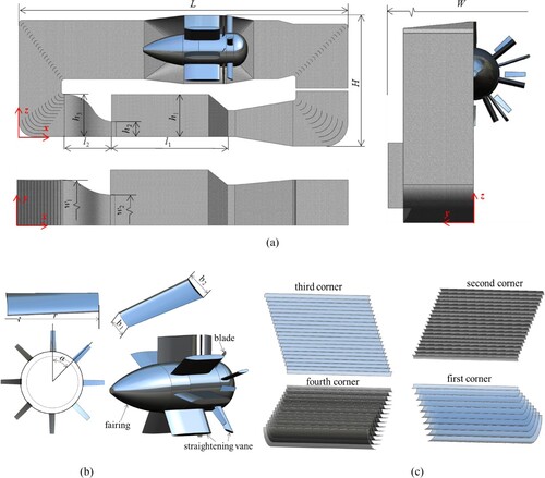
The simplified channel model of the RVISWT is illustrated in Figure 1, streamlining the representation by simplifying the ribbed plate on the channel wall and retaining only the flat surface within the channel. The overall geometric dimensions of the model, denoted as L, W, and H, are 21.65, 7.3, and 8.625 m, respectively. The specific dimensions of the test section, including length (l₁), width (w₂), and height (h₁), are 7.65, 7.3, and 2.8 m, respectively. In its original operational state, the air flow inlets h₂ and h₃ of the contraction section have heights of 2.8 and 1.0 m, respectively. The widths w₁ and w₂ are 6 and 4 m. The fan system has been simplified, retaining only the fairing, rotating blades, and stop vanes, as depicted in Figure 1(b). The radius (r) of the circle where the blade span is situated is approximately 2.25 m. The minimum and maximum widths (b₁ and b₂) are approximately 0.2 and 0.3 m, respectively, with eight fan blades evenly distributed at 45° intervals on the fairing. Deflectors at the four corners are depicted in Figure 1(c). The intricate refrigeration system within the wind tunnel is positioned behind the fan, aligning with the direction of the incoming flow. Furthermore, behind the diffusion section of the wind tunnel and preceding the flow of the refrigeration surface cooler, a snow-blocking net is present at the snow removal device. Notably, there are gaps on the wall of the wind tunnel connected to the outside in the vicinity of the snow removal device, resulting in a disconnected calculation domain at this location. Coordinate dimensions and velocities are denoted by x, u and u_p in the stream-wise direction, y, v and v_p in the span-wise direction, and z, w and w_p in the vertical direction. The coordinate origin is positioned in the symmetrical plane (span-wise direction) at the ground (vertical direction) and at the RVISWT's left outer wall (stream-wise direction), as illustrated in Figure 1(a).

Figure 1. Geometry of the RVISWT. (a) Full view of the RVISWT, (b) primary dimension of the fan system, and (c) configuration of the deflectors located at four corners of the RVISWT.

To investigate the influence of the shape of the contraction section curve on the flow characteristics of wind and snow within the test section, various contraction section curves are designed while maintaining a consistent contraction ratio. The spatial contraction section curves are illustrated in Figure 2, showcasing a symmetrical structure on the two lateral sides of the contraction in the width direction, where the contours on both sides of the curve mirror each other. Due to space constraints, the lower sides of the contraction are uncontrolled, forming a flat ground, and only the upper side is constructed. Vickers curves, bicubic curves, and quintic curves (Wang et al., 2022) are employed in this paper. Table 1 provides examples of the curve contours in both the top height direction and the width direction on both sides.

Figure 2. Contraction section curve definition. (a) Sketch of the contraction section, (b) configuration curves in the height direction, and (c) configuration curves in the width direction.

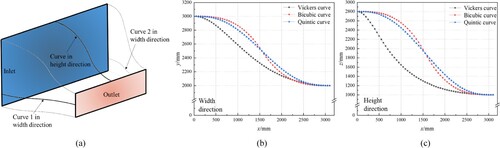
Table 1. Case definition for various contraction section curves.

Cases	Curve type at upper contraction	Curve type at lateral contraction
Case 1	Vickers curve	Vickers curve
Case 2	Vickers curve	Bicubic curve
Case 3	Vickers curve	Quintic curve
Case 4	Bicubic curve	Vickers curve
Case 5	Bicubic curve	Bicubic curve
Case 6	Bicubic curve	Quintic curve
Case 7	Quintic curve	Vickers curve
Case 8	Quintic curve	Bicubic curve
Case 9	Quintic curve	Quintic curve

The deflectors situated at the wind tunnel corners serve to guide the airflow, mitigate flow separation phenomena at the corners, enhance corner flow characteristics, and diminish the likelihood of uneven airflow or pulsations. However, the spacing of these corner deflectors significantly influences flow uniformity: smaller spacing results in more deflectors, leading to increased friction loss as the airflow passes through; conversely, larger spacing entails fewer deflectors, reducing friction loss but increasing eddy current loss due to corner flow. Despite these considerations, the introduction of discrete phase snow particles into the wind tunnel introduces an unknown element regarding the motion characteristics and accumulation distribution of these particles under different deflector arrangements. As a consequence, this paper is to scrutinize the distinctive characteristics of the discrete phase flow field within the wind tunnel, considering diverse deflector arrangements.

The selection of the deflector number at the channel's corners depends on specific criteria related to flow field quality and construction cost. This selection can be categorized into ‘Low-level’, ‘Medium-level’ and ‘High-level’ based on Equations (8)–(10) provided by Liu (2003), where S and C represent the chord lengths of the inner and outer arcs of the deflectors. The values of S/C at the third and fourth corners of the current RVISWT were measured as approximately 20.0 and 11.4, respectively. Using Equation (9), the medium-level deflector numbers at the third and fourth corners can be calculated as 28 and 16, respectively, which align with those of the existing RVISWT at Central South University. To further evaluate the effects of deflector layout density on wind-snow flow characteristics, the medium-level deflector numbers at the third and fourth corners are increased to a high level and reduced to a low level, respectively. These adjustments are based on the fixed values of S/C for the third and fourth corners. The calculated deflector numbers are rounded to integers and slightly adjusted for design convenience. The specific deflector numbers for the ‘Low-level’, ‘Medium-level’ and ‘High-level’ considered in this study are outlined in Table 2. It's important to note that, in this study, only the deflector numbers at the third and fourth corners are changed, while the deflector numbers at the first and second corners remain unchanged. (8) $\begin{array}{rl}{n}_{\mathrm{high}-\mathrm{level}}& =2.13\left(S/C\right)-1\end{array}$(8) (9) $\begin{array}{rl}{n}_{\mathrm{medium}-\mathrm{level}}& =1.4\left(S/C\right)\end{array}$(9) (10) $\begin{array}{rl}{n}_{\mathrm{low}-\mathrm{level}}& =0.9\left(S/C\right)\end{array}$(10)

Table 2. Number of deflectors at the corners of the RVISWT.

Cases	First corner	Second deflectors	Third corner	Fourth deflectors
Case 10: Low-level	9	18	19	12
Case 11: High-level	9	18	43	24
Case 12: Medium-level	9	18	28	16

2.3. Boundary condition

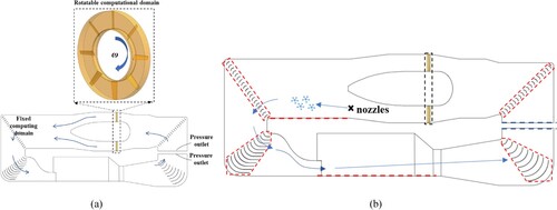
In this study, numerical simulation calculations are executed utilizing sliding grids, wherein a distinct rotatable computational domain is established around the eight blades and four pairs of exchange surfaces, as illustrated in Figure 3. The rotating computational domain revolves at an angular velocity denoted as ω = 30 rad/s, aligning the velocity at the test section inlet with the incoming flow velocity U_inf. Additionally, the velocity components in the stream-wise, span-wise and vertical directions of the airflow (u, v, w) and snow particles (u_p, v_p, w_p) in this study are all normalized using the incoming flow speed U_inf. The upper and lower surfaces of the right snow removal device are designated as pressure outlets. Here, the initial pressure (P) is set to 0 Pa, turbulence intensity (I) is set to 0.01, and turbulence intensity ratio is maintained at 10.0. Surfaces such as wind tunnel channels and corner deflectors are treated as fixed wall surfaces without sliding. In simulating the motion and accumulation of snow particles, specific boundary conditions are necessary for the RVISWT in numerical simulations. The lower walls downstream of the fan and within the test section, highlighted by red dashed lines in Figure 3(b), are designated as trap conditions. This indicates that snow particles are expected to accumulate on these surfaces without rebounding. Similarly, the corner deflectors highlighted by the red box in Figure 3(b) are also set as trap conditions to assess the effects of the deflector density on the snow accretion on these surfaces. The boundary surfaces between the rotating computing domain and the surrounding fixed computing domain, denoted by the black dashed box, are set as escape conditions. This signifies that particle trajectory calculations will be terminated upon encountering these surfaces. The snow removal device section, highlighted by the blue dashed lines, is also set as an escape condition. The remaining surfaces of the RVISWT's flow channel are considered reflect conditions, implying that snow particles will rebound off these surfaces upon impact.

Figure 3. Computational domain and boundary conditions. (a) Computational domain boundary condition for continuous phase, and (b) boundary definition for the discrete phase.

2.4. Computational grids

The computational domain is discretized by unstructured hexahedral volume grids. The trimmer technique in commercial software STAR-CCM+ is adopted for grid generation, as depicted in Figure 4(a). In order to capture the air flow within the boundary layer, 20 prism layers are applied to the surfaces of the channel and fan blades. The growth rate of the prism layer along the surface normal direction is 1.3, as shown in Figure 4(b). The surface mesh controllers are set for the primary components of the RVISWT, such as the blades, deflectors and channel, for a more flexible adjustment of the mesh resolution on these surfaces, as presented in Figure 4(c) and (d). The detailed size information of the coarse, medium and fine computational grids in the normal direction (y⁺= nU*/ν), stream-wise direction (s⁺= ΔsU*/ν), and span-wise direction (l⁺= ΔlU*/ν) is provided in Table 3. Notably, three sets of grids exhibit identical wall-normal distancing, ensuring that the mean value of y⁺ remains below 1.0 across the entire surface of the RVISTW.

Figure 4. Computational Grids. (a) Global mesh visualization for the RVISWT, (b) prism layers and spatial grids around the primary components, (c) surface mesh of the deflectors, and (d) surface mesh of the fan fairing and rotating blades.

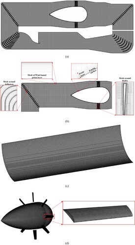
Table 3. Mesh resolution information for the coarse, medium and fine meshes.

		Blade			Channel			Deflectors
Resolution	Number	y^+	s^+	l^+	y^+	s^+	l^+	y^+	s^+	l^+
Coarse	32.5 million	0.9	468	468	0.9	532	532	0.9	522	522
Medium	68.5 million	0.9	266	266	0.9	282	282	0.9	332	332
Fine	102.4 million	0.9	132	132	0.9	156	156	0.9	164	164

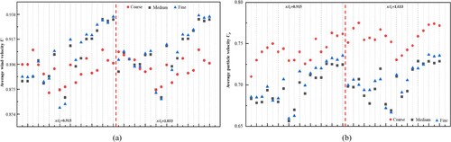
In order to elucidate variances in the dynamic characteristics of wind and snow within the test section under varying mesh resolutions, 36 monitoring points were strategically positioned, with detailed positional information provided in Figure 5. The time-averaged velocity magnitude values of both airflow and snow particles, as anticipated by different levels of mesh resolutions, are compared in Figure 6. The findings reveal that velocities for both airflow and snow particles at the monitoring sampling points are more closely aligned in medium and fine grids. Conversely, velocities projected by the coarse grids exhibit significant deviations from the outcomes of the other two mesh resolutions. This notable inconsistency implies that the resolution of the coarse grid falls short of meeting the requisites of the IDDES+ DPM method for effectively simulating the wind-snow flow dynamics within the RVICTW. In contrast, the medium grid scale not only demonstrates sufficient resolution accuracy but also exhibits robust consistency with the average velocities of the wind and snow derived from the fine meshes. Consequently, the medium grid resolution is deemed well-suited for the subsequent numerical investigation.

Figure 5. Layout of the monitoring points in the test section.

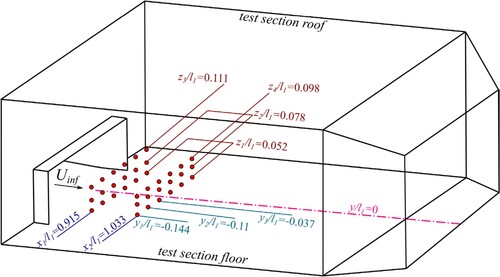
Figure 6. Comparison of the average velocity values of the airflow and snow particles at the monitoring points in the test section among the coarse, medium and fine grids. (a) Averaged velocity of airflow, and (b) Averaged velocity of snow particles.

2.5. Solver description

The numerical simulation is performed using the commercial fluid simulation software STAR-CCM+. Employing a separable incompressible unstructured finite volume solver, the coupling of pressure and velocity is achieved through the SIMPLE (Semi-Implicit Method for Pressure Linked Equations Consistent) algorithm. To discretize the convection term in the momentum equation, a mixed numerical scheme is employed, transitioning between the bounded central difference scheme (BCDS) utilized in the LES region and the second-order upwind scheme used in the RANS region. Simultaneously, the turbulence equation is discretized using the second-order upwind scheme. The time progression follows a second-order implicit format. The simulation employs an algebraic multigrid (AMG) linear solver, facilitating elastic cyclic solutions for both the momentum and turbulence equations.

To guarantee the accuracy and stability of the numerical simulations, each case undergoes an initial simulation using convergent RANS simulations to establish the flow field inside the wind tunnel. Subsequently, an unsteady-state simulation with a duration of T_adj= 2T_inf is conducted. This allows for the adjustment of the flow field, gradually transitioning from the steady-state RANS solution to the unsteady-state IDDES solution. Here, the reference time T_inf is defined as T_inf= L_f / U_ave, representing the time for incoming flow passages through the entire length of the RVICTW's channel (L_f) based on the averaged velocity (U_ave). Following this, an IDDES solution with a duration of $T_{\mathrm{sam}}^1=2T_{\inf }$ is performed, during which the first-order variables in the flow field are monitored and sampled. Finally, the IDDES solution with a duration of $T_{\mathrm{sam}}^2=2T_{\inf }$ is conducted, during which both first and second-order variables in the flow field are monitored and sampled. The chosen time step is set as Δt = 6.67 × 10⁻⁴T_inf for all simulations, ensuring a CFL number lower than 1.0 throughout the entire flow channel. The convergence criterions of the residuals of the continuity, momentum, turbulence and DPM equations were set as 10⁻⁵, and the maximum number of iterations is set to 30 to achieve appropriate convergence residuals and ensure the accuracy of the numerical simulation solutions.

In the present simulation, the heat and mass transfer during the formation of ice and snow particles, resulting from the interaction between atomized droplets expelled from the nozzle and the incoming frigid air, were not considered to save computational costs. Therefore, a simplification of simulated ice and snow particles becomes necessary. It is assumed that the snow particles maintain a spherical configuration without undergoing rupture or deformation after their ejection from the snowmaking nozzle. Interactions among particles are omitted, and a uniform internal temperature is assumed for each particle. Furthermore, any variations in the efficacy of snow particle dispersion among nozzles of the same model are disregarded, and the expelled supercooled droplets are assumed to exhibit uniform spraying speed and size. The number of snow particles ejected from the snowmaking nozzle at each time-step was set according to the fixed flow rate of 1 m³/h of the snowmaking devices. The discrete particles’ volume fraction within the flow field is constrained to be below 10%, making it suitable for simulation through the DPM method. The diameter and density of the snow particles applied in the numerical simulation are given as D_p= 40 µm and ρ_p= 250 kg/m³, respectively, selected based on the measured mean values of the snow particles ejected by the snowmaking devices of the RVICWT. The air density and dynamic viscosity of the airflow in the numerical simulations are selected according to the RVICWT's flow channel at the normal operating temperature of −20°C. Furthermore, a two-way coupling is established between the airflow and discrete phase particles, enabling momentum exchange between them during the simulation. These exchanged quantities serve as source terms for solving the continuous phase equation.

2.6. Validation

Wind tunnel tests were conducted in the test section of RVICWT to verify the numerical simulation adaptability of the IDDES turbulence model to the flow field characteristics of the ice and snow wind tunnel. Initially, flow field verification was conducted in the test section of the RVICWT to ensure the reliability of the obtained flow information. Cobra Probe was used to monitor velocity non-uniformity, turbulence level, directional angle, and dynamic pressure stability. Table 4 presents the comparison between the RVICWT's design values and the averaged values obtained from verification, indicating the reliable flow field quality within the test section and validating the predicting accuracy of the numerical method. Subsequently, the Cobra Probe was utilized to gather averaged velocity information within the test section of the RVICWT, as illustrated in Figure 7. Figure 5 depicts the spatial layout of sampling points for both numerical simulations and wind tunnel tests. The Cobra Probe operated at a sampling frequency of 2 kHz, with each sampling duration lasting no less than 100 s to ensure adequate convergence of stream-wise velocity data. The airflow velocity measurement was repeated at least three times per measurement point. Figure 8 compares the air velocities at sampling points in the RVICTW's test section, as predicted by the IDDES with SST k-ω turbulence model, with the corresponding average velocities measured using the Cobra Probe. The average velocity along the numerical simulation monitoring line closely matches the velocity values recorded by the Cobra Probe at each measurement point in the RVICTW's test section. Thus, it is evident that the flow field data obtained from the current numerical simulation, employing the SST k-ω turbulence model, accurately captures the key flow features within the RVISWT with a relative error of 1.2%. This demonstrates the high accuracy of the coupled numerical method of IDDES+DPM in predicting the continuous phase flow field in the RVICTW's channel.

Figure 7. Experimental setup for the velocity measurement in the test section of the RVISWT. (a) Testing plan of the velocity measurement, (b) Layout and installation of the cobra probe in the test section.

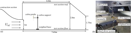
Figure 8. Comparison of the average velocity of the air flow in the test section between the numerical simulation and experiments.

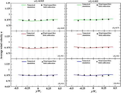
Table 4. Comparison of flow field calibration results.

Flow field parameters	RVICTW's design values	Verification's measured values
velocity non-uniformity	≤5.0%	3.5%
turbulence level	≤5.0%	4.5%
directional angle	Δα≤5.0°,	Δα = 3.36°,
	Δβ≤5.0°	Δβ = 4.23°
dynamic pressure stability	≤5.0%	3.83%

Additionally, wind-snow tests were carried out in the empty channel of the RVISWT to validate the accuracy of the coupled numerical method of IDDES+DPM in tracking the motion characteristics of snow particles, as illustrated in Figure 9. Each wind-snow test starts with approximately three hours of channel cooling operation, during which the fan speed is held at 5 rad/s. When the temperature reaches the experimental target of −20°C, the fan speed is then raised to the target speed of 30 rad/s for 20 min. Subsequently, the snow-making device is activated, and the flow rate for supplying water into the snow-making nozzle is set at 1 m³/h, the relative humidity in the test section of the wind-snow tests gradually reaches the target value of 85%. During the wind-snow test, environmental factors like temperature, humidity, and wind speed in the test section experience continual fluctuations, while in numerical simulations, these environmental variables remain constant. To ensure a more accurate comparison, maintaining the environmental variables as close to the target values as possible is crucial, as the environmental conditions in the wind tunnel have a significant impact on the motion trajectory and accumulation distribution of snow particles. Therefore, to ensure the stability of the test environment, the aforementioned parameters are monitored and sampled every 10 s throughout the entire wind-snow tests. In case of significant deviation, adjustments to wind tunnel environmental variables will be made promptly to maintain a stable and consistent testing environment. The key parameters for the wind-snow flow were maintained the same as those in the wind-snow tests during the validation simulation. Seven monitoring points were assigned to measure the snow accretion thickness on the channel floor, both upstream of the third corners and downstream of the fan system, as shown in Figure 9(a) and (b). Three wind-snow tests were performed under identical experimental conditions, during which the accumulated thickness at each measuring point was measured and averaged. Subsequently, these experimental results were compared to the numerical outcomes generated from the aforementioned IDDES+DPM method employing medium meshes.

Figure 9. Comparison of the snow accretion thickness on the channel's floor between the numerical simulation and wind-snow test. (a) Layout of the monitoring points for measuring the snow thickness, (b) snow accumulation on the channel's floor in the wind-snow test, and (c) quantitative comparison on the snow thickness between the numerical simulation and wind-snow test.

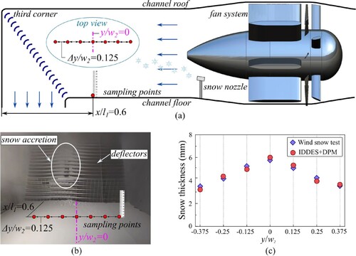
It is noteworthy that the continuous wind-snow testing duration (T_exp) extended to 600 times the reference time T_inf, significantly surpassing the numerical simulation time T_num= 6T_inf. This temporal dissonance is crucial in acknowledging the potential disparity in snow accretion thickness between the numerical simulation and the wind-snow test. The geometric configuration, boundary conditions, nozzle layout, and snow concentration in the validating numerical simulation were kept the same as the conditions of the wind-snow test in the RVISWT channel. This ensured that the snow particles would exhibit similar accumulation characteristics on the flat ground, characterized by a relatively constant speed in both the numerical simulation and the wind-snow test. Consequently, the snow accretion thickness predicted by the present numerical simulation was proportionally adjusted to align with the corresponding values within the same temporal frame as the wind-snow test, achieved by scaling the thickness by the ratio T_exp /T_num. In Figure 9(c), a comparative analysis is presented, contrasting the thickness values of snow accumulation at the designated monitoring points as predicted by the IDDES+DPM calculation against the measurements from the wind-snow test. Notably, the thickness values of snow accretion at the monitoring points exhibit a remarkable concurrence between the numerical simulation and the wind tunnel tests. The relative error of the IDDES+DPM calculation is confined to a mere 5.6%. The overall good agreement with the wind tunnel experiment (air velocity distribution in the test section and snow accumulation thickness on the channel's floor upstream the third corner) allows us to confidently select the IDDES+DPM method and medium mesh resolution to proceed with a more in-depth analysis of the results.

3. Results and discussion

3.1. Influence of contraction curve configuration on the airflow velocity distribution in test section

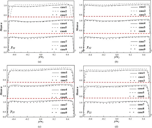
The velocity distribution within the test section, influenced by various contraction curves, is depicted in Figure 11. The horizontal monitoring lines’ positions in the span-wise direction are illustrated in Figure 10, denoting lines y₁₁, y₁₂, y₂₁, and y₂₂. The overarching observation from Figure 11 reveals that the spatial distribution characteristics of stream-wise velocity within the test section, under varying contraction curves, exhibit similarity. There is a relatively stable velocity value around u = 1.0 within the span-wise range of −0.4<y/w₂<0.4. Notably, the application of a bicubic curve at the lateral sides of the contraction imparts a pronounced accelerating effect, resulting in an elevated stream-wise velocity distribution. However, this acceleration also corresponds to a confined range of high-speed streamlines in the span-wise direction, as illustrated in Figure 11(a). In comparison to the bicubic curve, the implementation of a quintic curve at the lateral sides of the contraction demonstrates a more consistent behavior. Furthermore, when contrasted with the application of vickers and bicubic curves at the upper side of the contraction, the spatial distribution of stream-wise velocity induced by the quintic curve is more uniform. This indicates a more favorable influence of the quintic curve applied to the upper and lateral contraction on the flow field in the test section.

Figure 10. Layout of the sampling lines and planes in the test section for the numerical analysis.

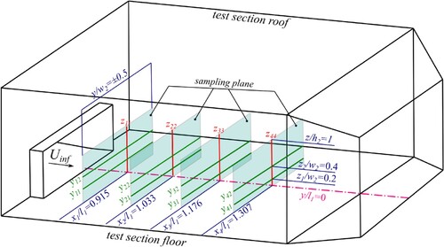
Figure 11. Averaged stream-wise velocity along different horizontal sampling lines in the test section. (a) y₁₂, (b) y₁₃, (c) y₂₂ and (d) y₂₃.

For a more quantitative analysis of the effects of contraction curves on flow characteristics in the test section, Table 5 compares dynamic pressure field coefficients at vertical sampling planes situated at stream-wise coordinates x/l₁= 0.915, 1.046, 1.176, 1.307. These sampling planes encompass the same span-wise and vertical range as the inlet of the test section. On one hand, when evaluating the curve types applied to the upper contraction, the comparison of dynamic pressure field coefficients in group 3 (cases 7, 8, and 9) reveals a significantly lower value compared to group 1 (cases 1, 2, and 3) and group 2 (cases 4, 5, and 6). This suggests a more favorable influence of the quintic curve at the upper contraction in controlling flow uniformity within the test section compared to the vickers and bicubic curves. On the other hand, in assessing curve types applied to the lateral contraction, it is evident that the vickers and bicubic curves lead to higher dynamic pressure field coefficients and poorer velocity uniformity inside the test section due to their excessively rapid contracting effect. Specifically, for cases with the same upper contraction curve, the application of the quintic curve to the lateral contraction proves beneficial in reducing dynamic pressure field coefficient values inside the test section compared to the vickers and bicubic curves.

Table 5. Comparison of dynamic pressure field coefficient.

	Dynamic pressure field coefficient
Case	x/l1 = 0.915	x/l1 = 1.046	x/l1 = 1.176	x/l1 = 1.307	Mean value
case1	1.96%	3.00%	2.51%	1.44%	3.23%
case2	2.09%	4.02%	3.39%	2.73%	3.06%
case3	2.41%	3.20%	3.05%	3.02%	2.92%
case4	2.55%	3.76%	3.70%	2.90%	3.23%
case5	2.32%	3.43%	2.87%	2.88%	2.87%
case6	2.57%	3.37%	2.70%	2.52%	2.79%
case7	2.18%	4.09%	3.32%	2.88%	3.12%
case8	2.10%	2.90%	2.47%	2.26%	2.64%
case9	2.54%	3.36%	2.57%	2.07%	2.43%

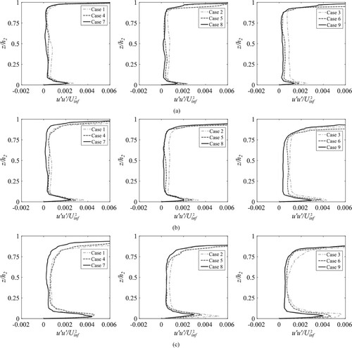
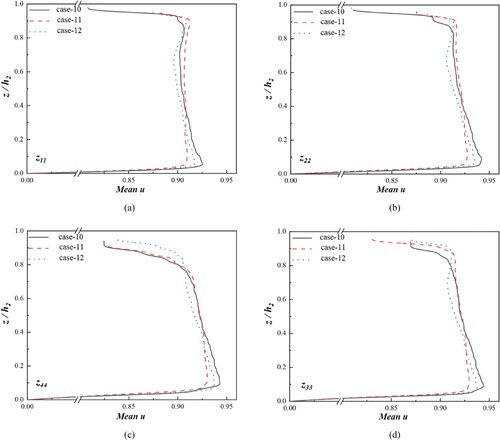
Figure 12 compares the time-averaged stream-wise normal stress distribution along the vertical sampling lines in the test section among all cases, aiming to offer a more quantitative analysis of the effects of the contraction curve configuration on the flow quality inside the test section. The general observation in Figure 12 indicates that the contraction configurations have a certain impact on the fluctuation of the velocity field inside the RVISWT's test section. The stream-wise normal stress values inside the test section are relatively low and close together, while the effects of the contraction configurations on the stream-wise normal stress are also noticeable. Specifically, for cases with the same lateral contraction configuration, it is observed that the quintic curve, when applied to control the upper contraction, significantly reduces the streamwise normal stress distribution inside the test section compared to the vickers and bicubic curves. Likewise, for the same upper contraction configuration, employing the quintic curve and vickers on the lateral sides of the contraction results in the highest and lowest streamwise normal stress levels, respectively. This discrepancy arises because the vickers and bicubic curves induce rapid compression, thereby enhancing the fluctuation of the velocity field during airflow acceleration in the streamwise direction. In contrast, the quintic curve offers a more stable compression process, consequently reducing the fluctuation level of the velocity field within the RVISWT's test section.

Figure 12. Averaged stream-wise normal stress distribution along different vertical sampling lines in the test section. (a) z₁₁, (b) z₂₂ and (c) z₃₃.

3.2. Influence of contraction curve configuration on the flow-deviation angle in test section

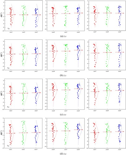
The flow deviation angles in the test section are crucial parameters for assessing the quality of the flow field in ice and snow wind tunnels. Therefore, this section compares the flow pitch angle Δα and yaw angle Δβ along the vertical monitoring lines z₁₁, z₂₂, z₃₃ and z₄₄, as depicted in Figure 10, to analyze the impact of various contraction section curves on the airflow direction in the test section. Figure 13 illustrates the distribution of the airflow pitch angle Δα on the vertical monitoring lines z₁₁, z₂₂, z₃₃ and z₄₄ in the test section. The horizontal red double-dotted lines in the figure represent the mean value of the airflow pitch angle on the corresponding monitoring line in each case, while the red, blue, and green dashed lines represent the normal distribution curve of the airflow pitch angle on the corresponding vertical monitoring line. The general observation in Figure 13 is that the vicker curve applied to the upper side of the contraction section results in a larger variance of the pitch angle, and the overall curve is chubbier, indicating a higher degree of pitch angle dispersion according to the normal distribution of the pitch angle. The corresponding variance of the bicubic curves is smaller, showing a lower degree of pitch angle dispersion. This is because the vickers curve has rapid compression in the vertical direction, and the airflow may diffuse upwards after passing through the nozzle of the test section. With the quantic curve applied to the upper contraction section, the pitch angle value significantly reduces, and the spatial distribution becomes more uniform due to the stable scale change in the vertical direction. In case 1, the averaged pitch angle along the four monitoring lines exhibits a notable elevation, registering a 31% increase compared to case 4 and a 9% upsurge relative to case 7. The mean pitch angle observed in case 2 surpasses that of case 5 by 1.4% and stands substantially higher, recording a significant 27% augmentation compared to case 8. In case 3, the mean pitch angle demonstrates a conspicuous ascent, presenting a 25% escalation in contrast to case 6 and a substantial 51% surge relative to case 9. Additionally, the application of the quantic curve to the lateral side of the contraction section (cases 7, 8, and 9) results in smaller values of the mean pitch angle than the vickers curve (cases 1, 2, and 3) and bicubic curve (cases 4, 5, and 6).

Figure 13. Distribution of pitch angle Δα along the vertical monitoring lines in the test section.

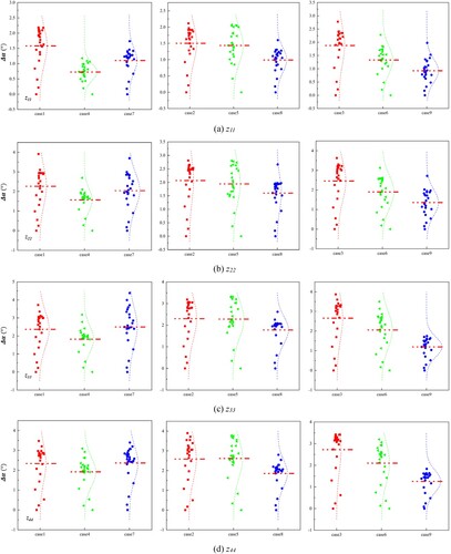
Figure 14 illustrates the yaw angle distribution along the vertical monitoring lines z₁₁, z₂₂, z₃₃, and z₄₄, within the test section. Within this dataset, cases 1, 4, and 7 exhibit vickers curves in the lateral contraction section, while cases 2, 5, and 8 present bicubic curves in the same section, and cases 3, 6, and 9 display quintic curves in the lateral contraction section. The corresponding curve types in each group adhere, sequentially, to vickers curves, bicubic curves, and quintic curves. On the whole, when the lateral curve of the contraction section assumes a vickers configuration (cases 1, 4, and 7), the absolute yaw angle of the airflow markedly exceeds that observed in the context of bicubic curves (cases 2, 5, and 8) and quintic curves (cases 3, 6, and 9). Notably, the adoption of quintic curves in the lateral contraction direction yields the lowest absolute yaw angle. Specifically, the averaged yaw angle in case 1 across the four monitoring lines is 13% lower than that of case 4 on average and 9% higher than that of case 7 on average. In the case of case 2, the mean yaw angle across the four monitoring lines is 6% higher than that of case 5 and a substantial 51% higher than that of case 8. Furthermore, the mean yaw angle in case 3 across the four monitoring lines registers a 29% increase compared to case 6 and a significant 38% elevation relative to case 9. Hence, it can be posited that when the lateral contraction curve assumes a vickers configuration, the swift compression of spatial scales on both sides prompts the airflow to diffuse towards both sides after traversing the test section. Conversely, the implementation of a quintic curve in the width direction results in a relatively flat slope in the contraction section compared to the other two curves, ensuring a stable scale change in the width direction. In turn, this contributes to a lower absolute yaw angle and substantially assures the quality of the flow field within the test section of the RVISWT.

Figure 14. Distribution of yaw angle Δβ of vertical monitoring line in the test section area.

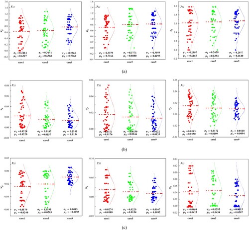
3.3. Influence of contraction curve configuration on the snow particles’ velocity distribution in the test section

Based on the preceding analysis of the flow field under distinct contraction section curve contours, it is evident that the flow field quality is superior under the influence of quintic curves, particularly in terms of velocity distribution and flow-deviation angle. Consequently, in this section, to delve more deeply into the streamlined study of snow particle distribution in the wind tunnel in a concise and efficient manner, we have selected three cases for comparative analysis: case 1 (employing vickers curves on the upper and lateral sides of the contraction section), case 5 (utilizing bicubic curves on the upper and lateral sides of the contraction section), and case 9 (employing quintic curves on the upper and lateral sides of the contraction section). In Figure 15, a comparison is drawn among the stream-wise velocity contours of snow particles in both the contraction section and the test section for case 1, case 5, and case 9. The sampling plane is strategically positioned at the middle center plane in the span-wise direction (y/w₂= 0). The overarching observation derived from Figure 15 is that the configuration of the contraction section exerts a substantial influence on the distribution of particle velocities in both the contraction section and the subsequent test section. Specifically, in case 1, the vertical distribution range of high-speed snow particle velocities is notably more confined compared to that in case 5 and case 9. Notably, case 9 exhibits the most extensive distribution range of high-speed snow particle velocities in the test section. This suggests that the incorporation of the quintic curve on the upper and lateral sides of the contraction section proves advantageous in mitigating the boundary layer effect exerted by the stationary ground on the motion of snow particles within the test section. In essence, the contraction section configuration governed by the quintic curve effectively simulates the wind-snow flow characteristics around a single bogie region under stationary ground conditions (Wang et al., 2018b, 2020).

Figure 15. Slices of mean velocity of snow particles in the ice and snow wind tunnel.

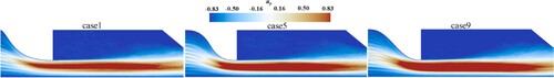
In Figure 16, a comprehensive examination of snow particles’ velocity components along the span-wise sampling lines y₁₁, y₁₂ and y₁₃ is conducted, comparing case 1, case 5, and case 9. The locations of these span-wise sampling lines are delineated in Figure 10. In the analysis presented in Figure 16(a), case 9 exhibits the highest mean value of stream-wise particle velocity with the lowest standard deviation when contrasted with case 1 and case 5. This suggests that the adoption of quintic curves to regulate upper and lateral contraction proves advantageous in enhancing the uniformity of snow particle flow and mitigating the boundary layer effects of stationary ground on particle motion in the stream-wise direction. This is particularly crucial for the test section with stationary ground when investigating snow accumulation on bogies. The significance lies in the fact that, in real operating scenarios of high-speed trains, there is no relative motion between the air and the subgrade, and no boundary layer is formed along the subgrade. Figure 16(b) and (c) reveal that the utilization of quintic curves (case 9) to control upper and lateral contraction markedly diminishes the absolute value of span-wise and vertical velocity of snow particles within the test section in comparison to vickers curves (case 1) and bicubic curves (case 5). This reduction indicates a noticeable decrease in the pitch and yaw angles of snow particles’ motion inside the test section due to the contraction controlled by quintic curves, owing to their consistent scale change in both the vertical and span-wise directions. Furthermore, standard deviation values of span-wise and vertical velocity of snow particles are significantly reduced in case 9 compared to case 1 and case 5. This reduction signifies that the contraction configuration characterized by quintic curves markedly enhances the flow uniformity of snow particles within the test section.

Figure 16. Distribution characteristics of the averaged velocity component of the snow particles on the vertical sampling lines of z₁₁, z₂₂ and z₃₃ inside the test section. (a) Averaged stream-wise velocity, (b) averaged span-wise velocity, and (c) averaged vertical velocity.

3.4. Impact of deflector numbers on the airflow characteristics inside the test

In the context of guiding airflow with deflectors in the RVISWT's channel, the quality of the flow field within the test section is substantially influenced and exhibits variations based on the arrangement of deflectors at different layout densities. To quantitatively assess the impact of deflector numbers on the flow field within the test section, an analysis is conducted, as depicted in Figure 17. The average stream-wise velocity of the airflow along the vertical monitoring lines z₁₁, z₂₂, z₃₃, and z₄₄ within the test section is illustrated, with the layout of the sampling lines provided in Figure 10. In comparing the averaged stream-wise velocity of the airflow, given the uniform contraction ratio in the contraction section, the airflow velocities from the nozzle in the three cases are similar, with the maximum velocity distribution occurring near the ground. Notably, within the range from z/h₂= 0.2 to z/h₂= 0.8, the mean stream-wise velocities exhibit relative stability across all cases. However, the entire velocity profile (u profile) in case 10 (fewest deflector number) noticeably inclines in the vertical direction, while it appears more uniform in case 11 (most deflector number). As the deflector number decreases to case 12 (medium deflector number), the u profile maintains spatial uniformity in the vertical direction, akin to what is observed in case 11. This suggests that employing more deflectors at the third and fourth corners enhances the flow quality within the RVISTW test section. However, this positive effect becomes constrained when the deflector number reaches a medium level in case 12.

Figure 17. Mean velocity in x direction of vertical monitoring line in test section.

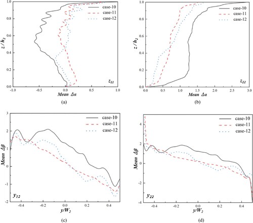
In Figure 18(a), the pitch angle distribution along the vertical monitoring lines z₁₁ and z₂₂ is compared, with their positions illustrated in Figure 10. Relative to case 10 (fewest deflector number), the incremental addition of deflectors at the third and fourth corners in case 11 (most deflector number) markedly reduces the absolute value of the pitch angle along the vertical monitoring lines z₁₁ and z₂₂. Furthermore, as the deflector number decreases to a medium level (case 12) from the highest level (case 11), the absolute value of the pitch angle does not exhibit a significant increase, maintaining a level comparable to that observed in case 11. On the other hand, Figure 18(b) presents a visualization of the yaw angle distribution along the span-wise monitoring lines y₁₂ and y₂₂. It is evident that case 11 exhibits the highest absolute values of the yaw angle among the three cases, while the absolute values of the yaw angle experience a substantial decrease in both case 12 and case 13. This reveals that increasing the deflector number at the third and fourth corners is advantageous in enhancing the quality of the flow field within the test section. Particularly noteworthy is the fact that within the range of y/w₂= ± 0.2, the average yaw angle in case 10 is 79% and 82% higher than that in case 11 and case 12, respectively. This quantitative comparison underscores that the average yaw angle value in case 12 closely aligns with that in case 11, indicating that the impact of increasing the deflector number on improving flow quality becomes limited as the deflector number reaches the medium level demonstrated by case 12.

Figure 18. Mean flow-deviation angle distribution along the monitoring lines in the test section. Pitch angles distribution along the vertical sampling lines (a) z₁₁ and (b) z₂₂. Yaw angles distribution along the span-wise sampling lines (c) y₁₂ and (d) y₂₂.

3.5. Impact of deflector numbers on the snow motion and accumulation distribution

As delineated in the foregoing analysis, the impact of the deflector number on the flow field quality is apparent – specifically, an increase in the number of deflectors contributes to a more uniform flow field in the deflector area. Nevertheless, the concomitant rise in blockage ratio introduces a potential impediment to the motion of snow particles and heightens the likelihood of snow particle accumulation on the deflectors. Consequently, the ensuing discussion explores the influence of the deflector number on the dynamics and spatial distribution of snow particles within the RVISWT.

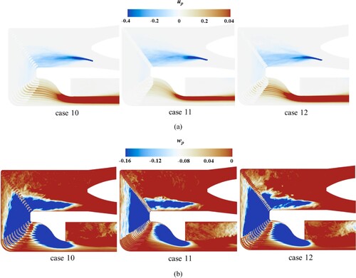
In Figure 19(a), the visualization of the stream-wise velocity distribution of snow particles around the third and fourth corners is presented. It is evident that case 10, with the lowest deflector number, appears to exhibit a wider range of high-speed snow particles in the test section compared to case 11, which has the highest deflector number. This phenomenon is primarily attributed to the significant increase in the blocking ratio of airflow and hindrance of snow particles as more deflectors are applied to the third and fourth corners. Consequently, this impediment allows fewer snow particles to reach the test section. Conversely, case 12 displays a distribution of high-speed snow particles in the vertical direction similar to that of case 10. Figure 19(b) provides a comparison of the vertical velocity distribution of snow particles near the third and fourth corners. The overall observation is that the number of snow particles reaching the test section after passing through the fourth corner in case 11 is the lowest, owing to the heightened blocking effect induced by the increased deflector number. In contrast, case 12 exhibits a snow particle distribution similar to that in case 10, indicating a limited influence of the increased deflector number on obstructing snow particles at the third and fourth corners, as the deflector number is lower than the medium level demonstrated by case 12. Furthermore, the vertical velocity distribution of snow particles in the test section in case 12 is nearly identical to that in case 10, with the absolute value slightly higher than that in case 11.

Figure 19. Averaged velocity components of snow particles around the third and fourth corners of the RVISWT. (a) Stream-wise velocity of snow particles, and (b) vertical velocity of snow particles.

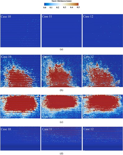
In the assessment of snow accumulation on the deflectors, Figure 20(a) provides a visualization of the snow distribution on the surfaces of the deflectors at the third and fourth corners. As observed in Figures 20(a) and (b), the lower surface of the deflectors at the third corner consistently exhibits more snow accumulation than the upper surface across all cases. This discrepancy arises due to the direct impact of snow particles on the lower surface. Moreover, the snow distribution range on the lower surface is smallest in case 10 and largest in case 11, corresponding to the lowest and highest blocking effects on snow particle motion in these cases. Regarding snow accretion on the deflectors at the fourth corner, the upper surface demonstrates significantly more snow accumulation than the lower surface. Although case 10 and case 12 exhibit more snow accumulation distribution than case 11 on the upper surface of the deflectors at the fourth corner, this observation may be attributed to the deflectors obstructing the snow accumulation on their downstream surfaces.

Figure 20. Distribution characteristics of snow accumulation on the deflectors located at the third and fourth corners of the RVISWT. Deflectors located at the third corners, (a) upper surface and (b) lower surface. Deflectors located at the fourth corners, (c) upper surface and (d) lower surface.

For a more precise and quantitative evaluation, Table 6 summarizes the mass of snow accumulation on the upper and lower surfaces of the deflectors at the third and fourth corners for all cases. The overarching observation in Table 6 is that case 10 and case 11 present the lowest and highest values of snow accretion mass on the deflectors at the third and fourth corners, respectively. Notably, in comparison to the total snow accumulation in case 10 (fewest deflector number), the total snow mass on the deflectors at the third and fourth corners increases by 57.8% in case 11 (most deflector number) and 17.8% in case 12 (medium deflector number), indicating a relatively limited influence of increasing deflector number on snow accretion mass between the lowest and medium levels of deflector numbers. However, the increasing deflector number on snow accretion mass becomes unignorable when the deflector number is between the medium level and the highest level. It is important to note that the mass values in Table 6 may seem low in all cases. However, extending the simulation time to the continuous testing duration of the RVISTW for 4 h (corresponding to the real operating time of the high-speed train on the Harbin-Dalian high-speed railway) would result in a considerable amount of snow accumulation on the deflectors of the RVISTW.

3.6. Suggestions for designing the ice and snow wind tunnel

The analysis above leads to the conclusion that the shape of the contraction section profoundly affects airflow quality and the motion characteristics of transported snow particles. Rapid compression of the contraction configuration results in turbulent airflow and snow particle movement, thereby reducing the quality of the wind-snow flow field in the test section. In real ice and snow wind tunnel designs, the contraction section design should adopt a smooth transition curve, considering cost and space limitations, to improve the flow field quality of the experimental section. It is noteworthy that the focus of the ice and snow wind tunnel in this study is primarily on investigating snow and ice accumulation on rail vehicle bogies. A turntable structure and wheelset drive system capable of supporting the actual bogie, which typically weighs around 10 tons, were installed in the test section. Consequently, the current vertical reflux ice and snow wind tunnel had limited space at the bottom for the contraction section, and the contraction curve was designed only for both sides and the top surface. In wind and snow experimental research involving other objects, quantic or smoother curves are recommended to control all surfaces of the contraction section, potentially leading to improved wind-snow flow quality within the test section.

Table 6. Snow accumulation mass on the deflectors located at the third and fourth corners of the RVISWT.

	Third corner deflector			Fourth corner deflector
Case	upper surface	lower surface	Sum	upper surface	lower surface	Sum	Total
case 10	0.089 kg	2.754 kg	2.843 kg	8.020 kg	0.002 kg	8.022 kg	10.865 kg
case 11	0.395 kg	6.206 kg	6.601 kg	10.541 kg	0.005 kg	10.546 kg	17.147 kg
case 12	0.167 kg	4.342 kg	4.510 kg	8.293 kg	0.003 kg	8.296 kg	12.806 kg

The density of the deflector layout plays a crucial role in shaping airflow quality and determining the distribution of snow particle accumulation. Although a high-density deflector layout enhances flow field quality, excessive density can lead to significant accumulation on their windward surfaces. Therefore, the study of deflector layout holds practical significance in actual ice and snow wind tunnel design, where selecting an optimal density is crucial for balancing flow field quality and snow accumulation on deflector surfaces. The presence of either too many or too few deflectors is not ideal. Therefore, it is recommended to adopt a medium-level deflector layout density for the design of the channel's corners of the RVISWT. Moreover, the ice and snow wind tunnel in this study did not address the issue of snow removal from deflectors during experiments. Implementing technologies for automatic snow removal from deflectors during wind-snow experiments could enable the use of more deflectors, thus enhancing wind-snow flow quality within the ice and snow wind tunnel's test section. This enables the assessment of the complete snow and ice accumulation process on the bogies of trains operating on long-distance alpine high-speed railways, such as the Beijing-Harbin High-speed Railway (approximately 6 h of continuous operation) and Lanzhou-Urumqi High-speed Railway (approximately 11 h of continuous operation).

4. Conclusions

This paper comprehensively investigates the effects of the contraction section configuration and the deflector layout density on the wind-snow flow characteristics within the test section of the Railway Vehicle Ice Snow Wind Tunnel (RVISWT). The investigation relies on the utilization of the improved Delayed Detached Eddy Simulation (IDDES) coupled with the Discrete Phase Model (DPM), validated against experimental data obtained from wind tunnel tests and wind-snow tests. The conclusions are summarized as follows:

1. The accuracy of the coupled IDDES+DPM method in predicting turbulent flow and tracking snow motion within the RVISWT is validated against experimental data, including velocity distribution within the test section and snow accretion thickness on the channel's floor. The IDDES+DPM approach adeptly captures key flow features within the RVISWT with a relative error of 1.2%, demonstrating commendable agreement between numerical results of velocity distribution and experimental data. Moreover, the IDDES+DPM method accurately forecasts snow accumulation on the channel's floor, with snow accretion thickness values showing remarkable alignment between numerical simulation and wind-snow tests. The relative error of the IDDES+DPM calculation is constrained to 5.6%. This overall good agreement verifies that the coupled method of IDDES and DPM with medium mesh resolution is a reliable tool for investigating wind-snow flow characteristics within an ice and snow wind tunnel. This provides a solid methodological foundation for the numerical investigation of wind-snow flow characteristics inside the ice and snow wind tunnel and for further optimization of channel configurations.

2. The effects of the contraction section configuration on wind-snow characteristics within the test section are elucidated, offering valuable insights into designing the contraction section for ice and snow wind tunnels. Specifically, compared to the vickers curve and bicubic curve, quintic curves applied to the upper and lateral sides of the contraction section consistently compress and accelerate airflow. This results in a more uniform flow characterized by lower stream-wise fluctuation levels, pitch angles, and yaw angles in the test section, thereby significantly improving the overall quality of the flow field. Furthermore, the contraction section controlled by quintic curves notably mitigates the boundary layer effects of the stationary ground on snow motion in the stream-wise direction. It demonstrates lower values of the span-wise and vertical velocity components of snow particles, leading to a more uniform velocity field for the snow particles compared to the vickers and bicubic curves. Consequently, it is recommended to utilize quintic curves or smoother curves in the design of the contraction section for ice and snow wind tunnels.

3. The influence of the deflector layout density on flow quality in the test section and snow accretion on the deflector are analyzed, providing insight into the reasonable arrangement of deflectors within the ice and snow tunnel. In particular, low deflector density results in a decrease in flow field quality in the test section, characterized by larger absolute values of pitch and yaw angles. Increasing the deflector number to a medium-level leads to a noticeable improvement in flow quality inside the test section. However, this positive effect becomes less pronounced with further increases in the deflector number. Conversely, the increasing number of deflectors significantly increases snow accumulation on the windward surfaces of deflectors, particularly at the third and fourth corners. Compared to scenarios with the fewest deflectors, the total snow accumulation mass increases by 57.8% with the highest deflector number, while it only increases by 17.8% for the medium deflector number. Therefore, a medium-level deflector density is recommended for designing ice and snow wind tunnels to achieve a better balance between flow quality and the additional snow accretion issue inside the channel.

Note that the current numerical method does not consider the phase transition process from supercooled droplets to snow particles. Interactions among particles are omitted, and the physical parameters of the snow particles are assumed to remain unchanged throughout the entire simulation. These factors are planned to be addressed in future numerical methods. With this methodological improvement, the key working parameters of the snow-making equipment and its spatial layout within the channel, as well as the configuration of the test section entrance, will be optimized to facilitate a higher flow quality of wind and snow in the RVISWT. Subsequently, the mechanism of snow and ice accumulation in the bogie region and effective anti-snow measures will be investigated using wind-snow tests for full-scale bogies in the RVISWT.

Data availability statement

The data that support the findings of this study are available from both the first author and the corresponding author upon reasonable request.

Disclosure statement

No potential conflict of interest was reported by the author(s).

Additional information

Funding

The research described in this paper was supported by the National Natural Science Foundation of China-China State Railway Group Co., Ltd. Railway Basic Research Joint Fund [grant number U2268217], the National Natural Science Foundation of China [grant number 52202429] and the Natural Science Foundation of Hunan Province of China [grant number 2023JJ40747].

References

- Allain, E., Paradot, N., Ribourg, M., Delpech, P., Bouchet, J.-P., de la Casa, X., & Pauline, J. (2014, March 24–26). Experimental and numerical study of snow accumulation on a high-speed train. 49th International symposium of applied aerodynamics.
- Baker, C. J., Quinn, A., Sima, M., Hoefener, L., & Licciardello, R. (2014a). Full-scale measurement and analysis of train slipstreams and wakes. Part 1: Ensemble averages. Proceedings of the Institution of Mechanical Engineers, Part F: Journal of Rail and Rapid Transit, 228(5), 451–467. https://doi.org/10.1177/0954409713485944
- Baker, C. J., Quinn, A., Sima, M., Hoefener, L., & Licciardello, R. (2014b). Full-scale measurement and analysis of train slipstreams and wakes. Part 2 Gust analysis. Proceedings of the Institution of Mechanical Engineers, Part F: Journal of Rail and Rapid Transit, 228(5), 468–480. https://doi.org/10.1177/0954409713488098
- Bansmer, S. E., Baumert, A., Sattler, S., Knop, I., Leroy, D., Schwarzenboeck, A., Jurkat-Witschas, T., Voigt, C., Pervier, H., & Esposito, B. (2018). Design, construction and commissioning of the Braunschweig Icing Wind Tunnel. Atmospheric Measurement Techniques, 11, 3221–3249.
- Barcelos, D. (2015). Flow quality testing and improvement of the Ryerson University low speed wind tunnel. Ryerson University.
- Cai, M., Gao, L., Liu, Z., Cheng, H., Wang, H., & Guo, Y. (2021). Experimental study on flow field quality of linear cascade wind tunnel under different conditions. Journal of Propulsion Technology, 42(5), 1162–1170.
- Chen, D. W., Sun, Z. X., Yao, S. B., Xu, S., Yin, B., Guo, D., Yang, G., & Ding, S. (2022). Data-driven rapid prediction model for aerodynamic force of high-speed train with arbitrary streamlined head. Engineering Applications of Computational Fluid Mechanics, 16(1), 2191–2206. https://doi.org/10.1080/19942060.2022.2136758
- Chen, G., Li, X. B., Liu, Z., Zhou, D., Wang, Z., Liang, X.-F., & Krajnovic, S. (2019). Dynamic analysis of the effect of nose length on train aerodynamic performance. Journal of Wind Engineering and Industrial Aerodynamics, 184, 198–208. https://doi.org/10.1016/j.jweia.2018.11.021
- Cheng, H., Wang, W., & Zhang, J. (2018). Nozzle jet flow field simulation of aerodynamic heating environment. Machinery Design Manufacture, 10, 5–8.
- Dong, T., Liang, X., Krajnović, S., Xiong, X., & Zhou, W. (2019). Effects of simplifying train bogies on surrounding flow and aerodynamic forces. Journal of Wind Engineering and Industrial Aerodynamics, 191, 170–182. https://doi.org/10.1016/j.jweia.2019.06.006
- Du, Q. (2017). Investigation on the methods of parameter measurement and calibration for small return-flow icing wind tunnels. Nanjing University of Aeronautics and Astronautics.
- Gao, G., Zhang, Y., & Wang, J. (2020). Numerical and experimental investigation on snow accumulation on bogies of high-speed trains. Journal of Central South University, 27(4), 1039–1053. https://doi.org/10.1007/s11771-020-4350-x
- Ghasemian, M., & Nejat, A. (2015). Aerodynamic noise prediction of a horizontal axis wind turbine using improved delayed detached eddy simulation and acoustic analogy. Energy Conversion and Management, 99, 210–220. https://doi.org/10.1016/j.enconman.2015.04.011
- Hu, D., Sun, K., & Zhang, Z. (2016). Testing and analysis of the flow quality of the low speed closed circuit wind tunnel. Journal of Shanghai University of Electric Power, 32(3), 211–215+220.
- Hu, P., Gu, Z., Bao, H., & Zhang, Q. (2013). Optimization of deflector layout parameters in wind tunnel based on flow field quality. Journal of Central South University (Science and Technology), 44(4), 1390–1396.
- Ju, L., Bai, J., & Guo, B. (2016). Effect of geometry parameters on flow field quality in a transonic slotted wind tunnel. Acta Aeronautica et Astronautica Sinica, 37(5), 1440–1453.
- Li, X. B., Chen, G., Wang, Z., Xiong, X.-H., Liang, X.-F., & Yin, J. (2019). Dynamic analysis of the flow fields around single- and double-unit trains. Journal of Wind Engineering and Industrial Aerodynamics, 188, 136–150. https://doi.org/10.1016/j.jweia.2019.02.015
- Liu, H., Niu, F., Niu, Y., Xu, J., & Wang, T. (2016). Effect of structures and sunny–shady slopes on thermal characteristics of subgrade along the Harbin–Dalian Passenger Dedicated Line in Northeast China. Cold Regions Science and Technology, 123, 14–21. https://doi.org/10.1016/j.coldregions.2015.11.007
- Liu, J., Liu, S., Xu, W., Wang, F., & Guo, P. (2017). Lubricant performance optimization and thermal banlance temperature analysis of high-speed train gearbox. Mechanical Drive, 4, 89–94.
- Liu, Z. (2003). Aerodynamic and structural design of high and low speed wind tunnels. National Defense Industry Press, 2003, 76–80.
- Ma, X., Zhang, C., Zhang, S., Ma, L., Zhou, P., & Zhang, X. (2015). The calculation methods of the high-speed train gearbox lubricant viscosity index. Lubrication Engineering, 4, 26–29.
- Menter, F. R. (2012). Two-equation eddy-viscosity turbulence models for engineering applications. AIAA Journal, 32(8), 1598–1605. https://doi.org/10.2514/3.12149
- Moustafa, A., Tarek, G., Chen, J. X., Elgamal, S., & Aboshosha, H. (2019). Designing a blade-system to generate downburst outflows at boundary layer wind tunnel. Journal of Wind Engineering and Industrial Aerodynamics, 186, 169–191. https://doi.org/10.1016/j.jweia.2019.01.005
- Shur, M. L., Spalart, P. R., Strelets, M. K., & Travin, A. K. (2008). A hybrid RANS-LES approach with delayed-DES and wall-modelled LES capabilities. International Journal of Heat and Fluid Flow, 29(6), 1638–1649. https://doi.org/10.1016/j.ijheatfluidflow.2008.07.001
- Wan, G., Soonho, S., Song, H., Kim, B., & Kim, K. (2023). Snow accretion on a model train: Climate wind tunnel experiments. Journal of Wind Engineering and Industrial Aerodynamics, 242, 105572. https://doi.org/10.1016/j.jweia.2023.105572
- Wang, J., Gao, G., Liu, M., Xie, F., & Zhang, J. (2018a). Numerical study of snow accumulation on the bogies of a high-speed train using URANS coupled with discrete phase model. Journal of Wind Engineering and Industrial Aerodynamics, 183, 295–314. https://doi.org/10.1016/j.jweia.2018.11.003
- Wang, J., Gao, G., Zhang, Y., He, K., & Zhang, J. (2019). Anti-snow performance of snow shields designed for brake calipers of a high-speed train. Proceedings of the Institution of Mechanical Engineers, Part F: Journal of Rail and Rapid Transit, 233(2), 121–140. https://doi.org/10.1177/0954409718783327
- Wang, J., Minelli, G., Dong, T., He, K., & Krajnović, S. (2020). Impact of the bogies and cavities on the aerodynamic behaviour of a high-speed train. An IDDES study. Journal of Wind Engineering and Industrial Aerodynamics, 207, 104406. https://doi.org/10.1016/j.jweia.2020.104406
- Wang, J., Wang, G., Xiong, B., & Sun, C. (2022). Simulation study on contraction curve of DC low speed wind tunnel. Henan Science and Technology, 41(22), 35–38.
- Wang, J., Zhang, J., Xie, F., Zhang, Y., & Gao, G. (2018b). A study of snow accumulating on the bogie and the effects of deflectors on the de-icing performance in the bogie region of a high-speed train. Cold Regions Science and Technology, 148, 121–130. https://doi.org/10.1016/j.coldregions.2018.01.010
- Wang, Y., Sun, Z., Ju, S., Guo, D., & Yang, G. (2023a). Robust optimisation of the streamlined shape of a high-speed train in crosswind conditions. Engineering Applications of Computational Fluid Mechanics, 17(1), 2234012. https://doi.org/10.1080/19942060.2023.2234012
- Wang, Y., Wang, T., Chen, J., Wu, Y., Zhao, C., Shi, F., & Tian, X. (2023b). Numerical study on slipstream-induced snow drifting and accumulation in the bogie region of a high-speed train passing the snowy ballast bed. Journal of Wind Engineering and Industrial Aerodynamics, 232, 105269. https://doi.org/10.1016/j.jweia.2022.105269
- Zhang, C., Xie, J., & Kong, Q. (2018). Characteristics of disastrous weather in Northeast China and its impact on railway transportation. Meteorological Disaster Prevention, 25(2), 33–36, 39.
- Zhang, D., Guo, Z., Ni, Y., Chen, Z.-W., Ao, W. K., Bordbar, A., & Zhou, F.-R. (2023). Correlation between cargo properties and train overturning safety for a high-speed freight train under strong winds. Engineering Applications of Computational Fluid Mechanics, 17(1), 2221308. https://doi.org/10.1080/19942060.2023.2221308
- Zhang, Y., Wang, J., Jiang, C., Zhang, J., Wang, T., & Gao, G. (2022). Investigation of ice and snow accumulations on the bogie areas of high-speed trains using ice wind tunnel experiments. Cold Regions Science and Technology, 199, 103560. https://doi.org/10.1016/j.coldregions.2022.103560
- Zhu, J., Hu, Z., & Thompson, D. J. (2016). Flow behaviour and aeroacoustic characteristics of a simplified high-speed train bogie. Proceedings of the Institution of Mechanical Engineers, Part F: Journal of Rail and Rapid Transit, 230(7), 1642–1658. https://doi.org/10.1177/0954409715605129