What are the appropriate mapping units for ecosystem service assessments? A systematic review

ABSTRACT

Context: Without clear understanding of the units used for ecosystem service (ES) mapping, ES assessment accuracy and the practical application of ES knowledge will be hampered. Method: We systematically reviewed 106 studies over the past 11 years to explore the type, characteristic pattern and deficiencies of mapping units. Result: We proposed that ES mapping units can be categorized into minimal unit for assessing ESs using corresponding indicators and methods, and aggregated unit for analysis and application based on research objectives, and classified the mapping units into five common types. Of the 12 characterizing variables of ES mapping studies, some have been shown to introduce a difference in the selection of mapping units and to exhibit characteristic patterns. We also found that the accuracy of ES assessments based on minimal units was lacking, and aggregated units were insufficient to establish a link between ES knowledge and practice. Conclusion: Herein, we propose possible solutions such as the use of fine spatial resolution grids and the introduction of additional data beyond land cover as supplements to improve the assessment accuracy. To enhance the availability of the results for practice, aggregated units connected with urban planning units should be established at a spatial level suitable for urban management.

KEYWORDS:

• Ecosystem service mapping
• ecosystem service assessment
• mapping unit selection
• systematic review
• minimal unit
• aggregated unit

Introduction

Ecosystem services (ESs) refer to the goods, services and environmental conditions that are indispensable for human well-being and subsistence that an ecosystem can provide while maintaining the integrity of its own ecological processes (Costanza et al. 1997; Burnett et al. 2006; Sannigrahi et al. 2019). Decision makers seeking sustainability should incorporate ES knowledge into practical operations, which has become a worldwide consensus. ES mapping can be an important tool to support policy makers and research institutions (Lorilla et al. 2019), enabling them to spatially identify which areas should be maintained because of their high supply of ESs by showing how values vary across space (Balvanera 2001; Martínez-Harms and Balvanera 2012).

Given the paramount importance of ES maps for decision making, there has been a rapid increase in the number of studies that map the spatial distribution of the ES supply (Martínez-Harms and Balvanera 2012). Some studies have reviewed the comprehensive progress of ES supply mapping. Englund, Berndes, and Cederberg (2017) and Maes et al. (2012) summarized the methods for mapping ESs at the landscape scale and in Europe to explore how to make ESs map better at the corresponding scale and scope. Andrew et al. (2015) reviewed nearly 150 studies, summarized five major paradigms for mapping ES supply, and identified representative data set types and sources. Martínez-Harms and Balvanera (2012) reviewed 70 articles that mapped the supply of ESs based on socioecological data. Crossman et al. (2013) reviewed additional articles not included in the review by Harms and Balvanera and found that regulating services have been most often mapped and climate regulation was the most commonly mapped ES.

We found that there are also some reviews addressing a specific aspect of the ES mapping procedure: Benis Egoh et al. (2012) summarized the ES indicators and available data sources used in ES mapping and modeling; Schägner et al. (2013) summarized the quantification methods for mapping the monetary value of the ES supply; and Malinga et al. (2015)reviewed the spatial scale and geographical coverage of different ES mapping studies. Some scholars also reviewed and evaluated the practice and application of specific ES mapping methods, such as the public participatory approach (Brown and Fagerholm 2015) and expert knowledge used for mapping ESs (Jacobs et al. 2015).

These reviews and the studies covered in them expressed the scholars’ desire to narrow the gap between the scholarly enterprise and the practical domains of ES assessment and mapping by finding more appropriate scales, data sources, indicators, methods and models. It is not enough for ES knowledge to satisfy the scholars’ interest in abstract problems only; moreover, it is necessary to establish a practical connection between ES research and planning and management practices that will be commonly recognized and applied by professionals committed to the swampy lowlands of practice (Schön 2001). Chen et al. (2019) evaluated the practice level of 76 ES mapping studies, and their conclusion tells us that there is an inadequacy in the outreach capacity of ES mapping research to make explicit connections with practice. Especially when the spatial scales and mapping resolution of ES maps do not match the social practical system, there would be a lack of incentives or adequate guidelines to use.

The spatial pattern of ES supply, demand and flow, the detection of ES hotspots and the division of ES bundles are highly dependent on the spatial resolution of the ES mapping unit. Spatial units in different forms and sizes represent fundamentally different aspects of the natural and socioeconomic systems (Holt et al. 2015). The choice of spatial units profoundly affects the conclusions drawn from ES assessment and mapping because the nature of these units determines the credibility of the spatial images. For example, the selection of ES quantitative indicators is closely related to pertinent spatial resolution (Syrbe and Walz 2012). Moreover, it is also critical to choose a method for delineating spatial areas in the research that is appropriate to the issues that are of concern to practitioners or their management decisions of interest because the nature and characteristics of the units determine their potential use for practical purposes (Kruczkowska, Solon, and Wolski 2017; Chen et al. 2019).

Although the spatial unit is of great significance for ES mapping and the transformation from research to practical applications, we found that, on the one hand, there are still a large number of ES mapping studies taking virtual grids with no boundaries in reality as the basic unit of mapping (Crouzat et al. 2015; Liquete et al. 2015; Jose Martinez-Harms et al. 2016; Spano et al. 2017; Vallecillo et al. 2018; Lorilla et al. 2019; Lyu et al. 2019), and such units without spatially explicit boundaries cannot accurately lie on the ground of the real world. On the other hand, the lack of a review of ES mapping units makes it difficult to know the achievements and implications of the studies that selected valid, practicably applicable ES mapping units with real boundaries.

Therefore, we pose the following questions in this paper:

• What types of units are used for ES mapping in existing studies?

• When selecting the basic unit for ES supply assessment, what factors related to ES calculations (such as indicators, data types and methods) should be considered to ensure mapping effectiveness?

• When selecting the unit for analysis and application based on quantified results, what factors related to practices (such as research objective) should be considered to ensure better connection between the research results and practical application?

Our research objectives are as follows:

• To establish a database to describe the types of units used in ES mapping research worldwide;

• To explore the factors affecting the selection of minimal and aggregated units and the characteristic patterns of different units; and

• To identify the deficiencies of ES mapping in unit selection, service assessment and practical application and propose possible solutions.

Materials and methods

Definitions and scope

We focused on ES supply, i.e., the capacity of a particular area to provide a specific bundle of ecosystem goods and services within a given time (Burkhard et al. 2012). This capacity represents the full potential of ecological functions or biophysical elements in an ecosystem to provide a potential ES (Tallis et al. 2011), irrespective of whether humans use or currently value that function or element (Martínez-Harms and Balvanera 2012). Identification of the key ecosystem service source areas would aid in ensuring continued delivery; this is why the study of ES supply mapping has been the focus of most studies to date (Martínez-Harms and Balvanera 2012).

Although the spatial units are heterogeneous, most ES assessment and mapping schemes require homogeneous units with distinct characteristics. Although ESs may be mapped at any desired resolution, this does not imply that the mapping unit is a viable ES-providing unit with ecological significance (Luck, Daily, and Ehrlich 2003). ESs emerge only when a minimum scale threshold is met (Nahuelhual et al. 2018). The ES mapping unit in this paper includes two kinds of units with different definitions and functions in the existing studies: one is the minimal unit for estimating the ES supply, which is regarded as a homogeneous spatial unit with a constant ES supply level in the calculation (Roces-Díaz et al. 2018b). The other is the aggregated unit used to further analyze and apply the quantitative results of ES supply assessment and mapping, which is obtained by integrating the minimal units and the calculated results on a specified spatial scope. According to the research and practical purposes, the scope of the aggregated unit may be the same or different from that of the minimal unit. Once the appropriate units have been established, the landscape structure, land-use composition or other biophysical attributes in each unit can be precisely quantified by selecting specific ES indicators (Syrbe and Walz 2012), and the ESs in the study area can be further analyzed and connected with the basic spatial units that are applied in practice.

Systematic review

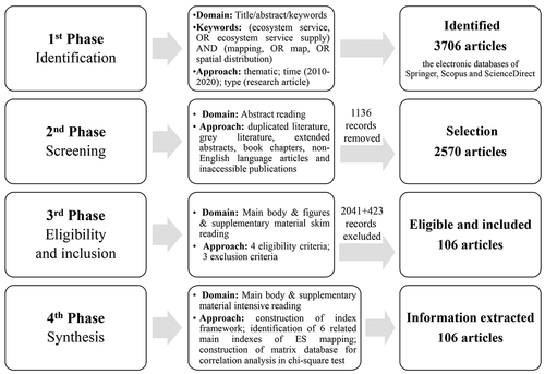
A systematic review is a review of a clearly formulated question using a systematic, explicit approach to identify, select, and critically evaluate the relevant research and to collect and analyze data from the source studies included in the review (Moher et al. 2010). The methodology used in this paper applied the main steps of the PRISMA (Preferred Reporting Items for Systematic reviews and Meta-Analysis) framework set forth by the Cochrane Collaboration (Moher et al. 2010; Sierra-Correa and Cantera Kintz 2015), 1) identification of articles via various databases and search engines; 2) screening of the identified articles to ensure their appropriateness for the research questions of this paper; 3) eligibility assessment in which prespecified eligibility and exclusion criteria had to be satisfied; and 4) extraction and classification of the relevant data from the selected articles to derive and synthesize information and knowledge. These steps are shown in Figure A.1.

Identification of the articles

Using the electronic databases of Springer, Scopus and ScienceDirect, the following terms (ecosystem service, OR ecosystem service supply, OR ecosystem service provision, OR ecosystem function[s]) AND (mapping, OR map, OR spatial distribution) were applied to titles, abstracts or keywords of articles in peer-reviewed journals about mapping ESs. Given the study purpose of providing up-to-date information, we focused on articles in the ES field with the fastest growth in the last eleven years (2010–2020) (Andrew et al. 2015; Chen et al. 2019). The initial search yielded a total of 3,706 articles.

Preliminary screening

By reading the articles’ abstracts and searching the full text, the number of articles was reduced to 2,570 for further eligibility assessment by removing duplicate articles, gray literature articles, extended abstracts, book chapters, non-English language articles and inaccessible publications. Because some research articles on the topic were not “open source” (approximately 1.1%), the final number of published articles for further assessment was limited.

Eligibility and exclusion

To determine how the articles fit the context of this paper, first, we skim read the full text of the article and its supplementary materials (if any), as well as the maps of ESs in the article, and applied four eligibility criteria (Table 1) to screen the articles. As a result, 2,041 articles were deleted because of irrelevance to this review. Second, articles were deleted based on three exclusion criteria (Table 1). A total of 106 SCI articles fulfilled the criteria, accounting for 2.9% of the initial articles in the database (Table A. 1).

Table 1. The eligibility and exclusion criteria for published articles

Eligibility criteria	Reasons for or types of excluded article
1) The study had a connection to a case study, such as a plan, design, construction, restoration and management.	The study focused on conceptual or theoretical frameworks of ES mapping; the study purely focused on methodological or technical improvements.
2) The study was conducted in a terrestrial ecosystem.	The study was conducted in a marine ecosystem.
3) The study used a specific biophysical or socio-ecological indicators, or mapped ES supply using methods based on specific information about ecosystem structure, composition, and ecological processes.	The study used participatory mapping as the method (based on questionnaires and interviews); or the study used the value transfer method or equivalent factor method to map ESs based on the unit area value of specific land use type.
4) The study presented spatially explicit quantification of ESs at a lower level than global.	The study used the mapping and analysis unit at a higher level than national.
Exclusion criteria
1) The study did not provide clear data sources and assessment methods for ES supply.
2) The study lacked clear elaboration of ES supply mapping method and presentation of mapping results.
3) The study mapped and analyzed ES supply based only on grid cells with virtual boundaries.

Information extraction and synthesis

We used an index framework to extract and organize the relevant information on mapping unit selection from the 106 SCI articles in an Excel spreadsheet. In addition to the basic information (number and article title), the framework includes six major indexes and their 18 subcomponents. Among them, 12 variables describe the characteristics related to the ES mapping study, and six variables describe the characteristics of the mapping unit: I) characteristics of the study area: study level, mapped area and prominent landscape feature; II) characteristics of the minimal units: type of unit, type of unit boundary and unit extent; III) characteristics of the aggregated units: type of unit, type of unit boundary and unit extent; IV) characteristics of the mapped ESs: number and type of the ESs studied and type of ES indicators; V) characteristics of the research method: type of data source, mapping resolution and ES quantification and mapping method; and VI) characteristics of the application and practices: type of practical objective, type of further analysis based on ES mapping and type of practice to support (see Table A. 2 for detailed explanations of the index and variable values).

To conduct qualitative and quantitative analyses, we establish a matrix database following an iterative process of coding the materials (Yin 1993). More than one type of minimal unit or aggregated unit may be used in an article. If an article was selected for review, all ES mapping units used in the article were recorded as separate entries in the matrix, and other information corresponding to each mapping unit was also recorded separately. If two articles used exactly the same type of mapping unit, each was considered individually and was treated as representing two distinct data items. By these means, we obtained a matrix database with 114 (number of mapping units selected in the review articles) × 27 (variables, value under the six main indexes) (Table A. 3). There were two types of variables: three continuous variables: the mapped area, number of ESs studied and mapping resolution; and 24 category types, such as prominent landscape features and type of practical objective.

Since 89.0% of the variables were defined on a nominal scale and have characteristics that cannot be quantified (Gilbert and Prion 2016), we conducted the Pearson chi-square test on the variables to analyze whether there is a statistically significant difference between the expected and observed values in the distribution of the two variables (Luna-Romera et al. 2019). The purpose was to explore whether the selection of ES mapping units in each article varied according to the variables describing other characteristics of the study. The Pearson chi-square test is a nonparametric analysis technique providing hypothesis tests for qualitative data when there are categories instead of numbers (Siegel 2012). Monte Carlo permutation tests with 999 permutations were performed to generate p values that are used to evaluate the significance of the relationships between the variables (TerBraak and Smilauer 2012); the correlation degree between the two variables was tested by Cramer’s V coefficient (0–1), which was weak if less than 0.3 and strong if greater than 0.6 (Babu and Sanyal 2009). The matrix database (114 × 27) obtained from the 106 reviewed articles (Table A. 3) was entered into SPSS 18 software as the original data to perform the Pearson chi-square statistical test and treatment at the level of 0.01 (Arbuckle 2012).

Technical definitions of the indexes and variables in the matrix databases

Different landscape features in the study area may influence the selection of mapping units. Some articles explicitly pointed out the dominant landscape type(s) of the study area by using phrases such as “dominated by … ” and “primarily used for …, ” or they clearly showed a significant proportion of land or landscape through data and land use and land cover (LULC) maps. Studies of specific ecosystems (forests, water bodies, cities, etc.) can also clarify this. We collected and summarized this information in the index framework.

The Common International Classification of Ecosystem Services (CICES, V 4.3) published at the beginning of 2013 is widely used in current studies (Haines-Young and Potschin 2013). In the design of CICES V4.3, ESs are classified into three types: provisioning, regulating and cultural. In contrast to the Millennium Ecosystem Assessment (2005), supporting services are not included in this classification since the focus was on how ecosystem outputs more directly contribute to human well-being (Czúcz et al. 2018). To avoid double-counting and to take into account that some studies do not specify the type of service, such as Mexia et al. (2018), we classified the services into the three types designed by CICES.

Existing reviews classified ES indicators according to the service types they assessed (Benis Egoh et al. 2012; Fagerholm et al. 2012), their data properties (Chen et al. 2019) and spatial characteristics (Andrew et al. 2015). In this paper, we divided ES indicators into three categories according to their attributes (Seppelt et al. 2011): biophysical, socioeconomic and categorical indicators. For ES quantification and mapping methods, we integrated the existing classification of many reviews (Seppelt et al. 2011; Benis Egoh et al. 2012; Martínez-Harms and Balvanera 2012; Andrew et al. 2015; Englund, Berndes, and Cederberg 2017; Chen et al. 2019) and divided the methods into four categories according to the main methods of mapping: direct, empirical, model and proxy mapping.

With the definition of the five common human activities related to nature in Xiang (2017), combined with the actual situation of the reviewed articles, we divided the practice types supported by ES mapping research into four categories: planning, design, restoration/conservation, and management. In addition, we classified the extent of the ES mapping unit qualitatively according to an estimation of the area size, which serves as a descriptive reference for the unit’s characteristics. This is because most studies do not provide data or information that allowed us to quantify the area of a mapping unit.

Results

Types of minimal units for ES mapping

Among the 114 mapping units selected in the 106 articles, studies using land-use units and grid cells as the minimal mapping units for ESs were the most common, accounting for 30.7% and 29.0%, respectively. Administrative/management units, geographical/biophysical units and units with specific planning/design/analysis intent followed with 15.8%, 13.2% and 11.4%, respectively. The highest proportions of the minimal unit extent were site level (30.7%) and patch level (46.5%).

The land-use units were classified according to the land-use map or regional land cover data set using the existing planning boundary of land-use patches. Grid cells were generated by ArcGIS spatial analysis technology based on raster maps. The extent of the grid cells used in the articles varied from 10 m × 10 m to 1 km×1 km and were of two types: rectangular (97.0%) and hexagonal (3.0%). The administrative/management unit refers to a region defined by a political boundary. Corresponding to different administrative levels and management subjects, administrative/management units used in the articles included forest management units (5.3%), blocks (15.8%), townships (15.8%), counties (21.1%), municipalities (36.8%) and provinces (5.3%). The units’ extent covered local and regional levels. Geographical/biophysical units were derived from the spatial classification of a series of biological, physical, and geographical characteristics of the study area. The unit boundaries exhibited highly geographical/biophysical features. This type included a homogeneous landscape/ecosystem unit (26.7%), homogeneous vegetation feature unit (46.7%) and small watershed unit (26.7%). The unit extent covered site, patch and region.

Some articles selected units with specific planning or design intent using existing planning or design boundaries in reality, including urban green roofs (7.7%) and various forms of urban green spaces (53.8%). Other articles defined their own spatial units with specific meanings (38.5%). For example, Mexia et al. (2018) used vegetation planting units based on the type and structure of vegetation planted in the park as the basic unit. By identifying and extracting ES service provisioning elements such as terrace gardens, algal pools, green walls and greenhouses on buildings in the city, Kain et al. (2016) introduced more details to urban green patches. The minimal units of this kind were used to a small extent, such as sites or patches.

Types of aggregated units for ES mapping

Among the 106 articles, some selected different minimal and aggregated units to assess and analyze ESs, respectively; 45.6% of them were inconsistent in type (Figure 1). Most of these studies (86.5%) were carried out at relatively high levels, such as municipal and above.

Figure 1. A statistical comparison of the selection of minimal and aggregated unit types in the sampled studies

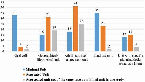
The most common types of minimal units that were integrated were grid cells and land-use units, accounting for 59.6% and 26.9% of the total number of inconsistencies, respectively. Among all aggregated units that were not of the same type as the minimal units, the administrative/management units were chosen most often, accounting for 48.1%. Geographical/biophysical units (36.5%) were next, and units with specific planning/design/analysis intent, grid cells and land-use units were the least common, accounting for 7.7%, 3.8% and 3.8%, respectively.

We mainly counted the aggregated units that were not of the same type as the minimal units. The administrative/management units consisted of five categories: ecoregions and protected areas (14.3%), neighborhoods (14.3%), townships (13.6%), counties (21.4%) and municipalities (46.4%), of which 16.0% involved multiextent research. Geographical/biophysical units included (sub)watershed units (78.9%) and homogeneous landscape/ecosystem units (21.1%), with local and regional study levels. The units with specific planning/design/analysis intent had three extents: the urban structure unit (25.0%) at the site level, the urbanization level zoning (25.0%) at the local level, and the socioeconomic unit (50.0%) at the regional level. The first one borrowed the existing spatial planning boundaries to define the units (Wurster and Artmann 2014), and the last two identified units based on similarity analysis of urbanization level, social, economic and cultural characteristics and land-use types, combined with the administrative divisions (Li et al. 2016a; Zhang et al., 2017a; Castillo-Eguskitza, Martín-López, and Onaindia 2018).

Using grid cells at a higher level, Xu et al. (2017) aggregated the grid cells for ES assessment at the lower level to observe the correlation between different ES pairs and spatial patterns and aggregation characteristics of ESs on a continuous spatial scale (1 km×1 km – 20 km×20 km). In addition, when the land-use unit was taken as the aggregated unit, relevant articles used it to aggregate the minimal units of the grid cell type (Koschke et al. 2014; Zarandian et al. 2017).

Variables affecting the selection of minimal units

We identified the variables that were moderately and strongly correlated with the minimal unit (Cramer’s V coefficient >0.3) that passed the significance test at the 0.01 level (Table 2). The results show that:

Table 2. The Sig value and Cramer’s V between variables with significant relationships in Chi-square Test

Variable 1	Variable 2	Sig. (<0.01)	Cramer’s V (>0.3)
Type of minimal unit	Prominent landscape feature	0	0.334
	Number of studied ESs	0	0.385
	Type of studied ESs-provisioning	0.005	0.364
	Type of ESs indicators-biophysical	0	0.432
	Type of ESs indicators-socio-economic	0	0.443
	Type of ESs indicators-categorical	0	0.506
	Type of data source-socio-economic	0.003	0.372
	Type of data source-qualitative/expert	0	0.455
	ES method- direct/primary	0.003	0.379
	ES method- empirical	0	0.54
	ES method- model	0.002	0.392
	ES method- proxy	0.003	0.375
	Type of practical objective	0	0.427
	Type of practice to support	0.002	0.33
Type of minimal unit boundary	Number of studied ESs	0.002	0.306
	Type of ES indicators-biophysical	0.002	0.365
	Type of ES indicators-socioeconomic	0.004	0.34
	Type of ES indicators-categorical	0	0.498
	Type of data source-socio-economic	0.003	0.351
	Type of data source-qualitative/expert	0	0.447
	ES method- direct/primary	0.005	0.337
	ES method- empirical	0	0.476
	ES method- model	0.001	0.38
	Type of practical objective	0.001	0.314
	Type of further analysis based on ES mapping	0.004	0.312
Minimal unit extent	Number of studied ESs	0.004	0.314
	Type of ES indicators-biophysical	0.004	0.37
	Type of ES indicators-socioeconomic	0.001	0.41
	Type of ES indicators-categorical	0.002	0.387
	Type of data source-qualitative/expert	0.007	0.35
	ES method- direct/primary	0.003	0.371
	ES method- empirical	0	0.42
Type of aggregated unit	Number of studied ESs	0.001	0.338
	Type of studied ESs-provisioning	0.008	0.349
	Type of ES indicators-categorical	0.007	0.35
	Type of data source-biophysical	0.004	0.364
	Type of data source-qualitative/expert	0.004	0.369
	ES method- empirical	0.001	0.414
	Type of practical objective	0	0.387
	Type of practice to support	0.004	0.3
	Type of studied ESs-cultural	0.005	0.335
	Type of ES indicators-categorical	0.009	0.32
Variable 1	Variable 2	Sig. (<0.01)	Cramer’s V (>0.3)
Type of aggregated unit	Type of data source-qualitative/expert	0.007	0.339
	ES method- empirical	0.007	0.325
	Type of practical objective	0	0.323
Aggregated unit extent	Study level	0	0.328
	Mapped area	0	0.354
	Prominent landscape feature	0	0.37
	Type of ES indicators-biophysical	0.004	0.369
	Type of data source-biophysical	0.01	0.341
	Type of data source-qualitative/expert	0.006	0.354
	ES method- empirical	0.001	0.41
	ES method- proxy	0.009	0.343
	Type of practical objective	0	0.363
	Type of further analysis based on ES mapping	0.003	0.302
	Type of practice to support	0	0.334

1) Among the variables related to the characteristics of the study area, the prominent landscape feature was correlated with the type of minimal unit, which means that the difference in landscape features would lead to the difference in the selection of minimal unit type (Figure 2-a).

Figure 2. The relationship between the minimal units and their influencing variables

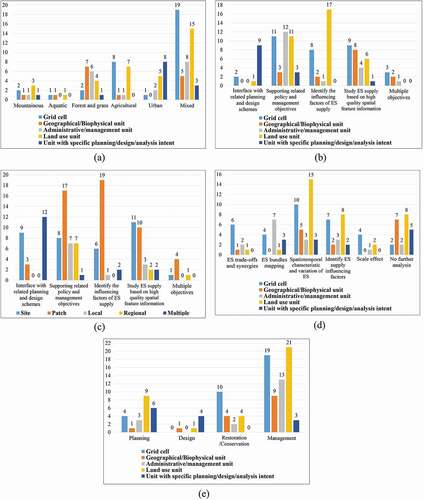
2) Among the variables related to the characteristics of the mapped ESs, when the number of ESs was less than 10, the most commonly used minimal units were grid cells with virtual boundaries (36.4%) and the cell extent at the patch level (39.8%). When the number of ESs was greater than 10, the patch-level land-use units were most often used as the minimal unit (69.2%). When mapping the provisioning services, the most commonly used were grid cells (32.1%). When using biophysical indicators, the most commonly used were grid cells (33.7%) with virtual boundaries and the extent of the site and patch levels (37.1% each). When using socioeconomic indicators, the most commonly used were grid cells (32.2%) with virtual boundaries and the extent of the site level (37.3%). When using categorical indicators, the most commonly used were the land-use units (61.8%), the boundary generated by planning/design/analysis (79.4%), and the unit extent of the patch level (73.5%).

3) Among the variables related to the characteristics of the research method, when using socioeconomic data, grid cells with virtual boundaries were the most commonly used (36.1%). When using qualitative/expert data, there was a significant tendency in the selection of land-use units with planning and design boundaries at the patch level (58.1%). Administrative/management units with political boundaries were most commonly used (31.7%) when using direct mapping based on primary data. When empirical mapping was used, the land-use units at the patch level (68.8%) were most frequently used. When using models and proxies, grid cells with virtual boundaries were used most often (40.0% and 42.5%, respectively).

4) Among the variables related to the characteristics of application and practice, the application and practice objectives of the studies were correlated with the type (Figure 2-b), boundary and extent (Figure 2-c) of the minimal unit, in which the selection of type and boundary showed corresponding and consistent differences. The selection of the minimal unit type varied with the different directions of the further analysis (Figure 2-d), and the selection of the boundary also showed correspondingly consistent differences. The different types of practice supported by the studies impacted the selection of the minimal unit type (Figure 2-e).

Variables affecting the selection of aggregated units

We identified the variables that were moderately and strongly correlated with the minimal unit (Cramer’s V coefficient >0.3) that passed the significance test at the 0.01 level (Table 2). The results show that:

1) Among the variables related to the characteristics of the study area, the study level and mapped area were positively correlated with the extent of the aggregated unit; the higher the study level and the larger the mapped area, the larger the extent of the selected aggregated unit. The prominent landscape features in the study area were correlated with the extent of the aggregated unit and led to differences in selection (Figure 3-a).

Figure 3. The relationships between the aggregated units and their influencing variables

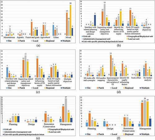
2) Among the variables related to the characteristics of the mapped ESs, when the number of ESs was less than 10, geographical/biophysical units and administrative/management units were the most commonly used (34.1% each). When the ES number was 10–20, the administrative/management aggregated units were most commonly used (50.0%). When the ES number was greater than 20, land-use units were the most common aggregated unit (66.7%). The most frequently used aggregated unit for the mapping of provisioning and cultural services was the administrative/management unit with political boundaries (41.7% and 45.5%, respectively). When using categorical indicators, land-use units with boundaries generated by planning/design/analysis were the most frequently used (38.2%).

3) Among the variables related to the characteristics of the research method, when using biophysical data, administrative/management units were the most commonly used aggregated unit (38.0%), and the local level was the most commonly used (32.0%). When using qualitative/expert data, land-use units with boundaries generated by planning/design/analysis at the patch level were the most common aggregated unit choices (41.9%). When using empirical mapping methods, land-use units with boundaries generated by planning/design/analysis at the patch level were most commonly selected (43.8%).

4) Among the variables related to the characteristics of the application and practice, the application and practice objectives of the studies were correlated with the type (Figure 3-b), boundary and extent (Figure 3-c) of the aggregated unit, in which the selection of the type and boundary showed corresponding and consistent differences. The selection of the aggregated unit extent varied with the different directions of further analysis (Figure 3-d). Different types of practice supported by the studies had an impact on the selection of the aggregated unit type (Figure 3-e) and extent (Figure 3-f), representing certain otherness characteristics.

Discussion

Different types of minimal units showing different priority and characteristic patterns

According to the selection of the minimal mapping unit in the review articles, grid cells and land-use units (29.0% and 30.7%, respectively) showed certain advantages. A rectangular grid is a common unit for ES assessment with a high resolution or at a high study level, which can show a high degree of spatial pattern heterogeneity (Roces-Díaz et al. 2018a). It is often used to unify the units of different ES proxies or indicators, as well as the resolution of acquired data (Crouzat et al. 2015; Liquete et al. 2015). In addition, studies have shown that the hexagonal grid is a more appropriate spatial discretization scale than the former when evaluating specific types of ESs (Lorilla et al. 2018). For local climate regulation services, for example, this discretization scale represents the estimated spatial reach of local air flow that redistributes heat and mixes local air temperatures, thus allowing the local climate regulation services provided by the mixed air to be calculated within each spatial unit (Goldenberg et al. 2017). Land-use units suggest place-based assessment. Many studies combine LULC proxies with the supply level per unit area of the ESs (Schägner et al. 2013), evaluated through direct-mapping methods based on empirical mapping on the basis of expert scoring. This makes it possible to evaluate ESs in data-scarce regions (Vrebos et al. 2015), and it is beneficial to monitor the impact of land-use changes on ESs (Kreuter et al. 2001; Mendoza-González et al. 2012).

Considering the availability of data and the selection of ES indicators, the administrative/management unit is the finest scale for official statistics (Roces-Díaz et al. 2017; Lin et al. 2018), and a political boundary is suitable for identifying the major drivers of supply and demand changes of ESs in a social ecosystem (Zhang et al. 2017b; Cui et al. 2019). Selecting a geographical/biophysical unit as the minimal unit is often out of high concern for the heterogeneity of the landscape space, thus enhancing the analysis and interpretation of the quantitative results (Yaneva 2016; Roces-Díaz et al. 2017). Units with specific planning/design/analysis intent are based on a parcel-based ES assessment and mapping approach (Chen et al. 2019). Unlike large geographical/biophysical units that rely solely on general landscape feature differentiation, the minimal units at the site and patch levels explore the details of ES provisioning and consumption within the units, which are useful for assessing the ESs provided by the landscape at a high resolution.

By using a chi-square test, we found that a series of variables made a difference in the selection of the minimal unit, including variables describing the characteristics of the study area, such as prominent landscape features, and the variables representing the characteristics of application and practices, such as the practical objectives, further analysis based on ES mapping and the type of supporting practice. In addition, certain types of descriptive variables for the characteristics of the mapped ESs have also been shown to influence the selection of minimal units, such as ES indicators, data types and mapping methods. These results remind us that when the study of ES mapping involves the use of the above variables, the selection of the minimal unit has specific patterns. These patterns for each type of minimal unit have been shown to be available and effective for existing successful practices and are summarized in Table 3. These patterns can be used as references for selecting an appropriate and effective minimal unit for ES mapping under specific research characteristics and conditions.

Table 3. The characteristic patterns in each type of minimal unit (as selection references)

Frequency	Type of minimal unit	Variable delineating characteristic patterns of minimal units
		Study level	Mapped area	Prominent landscape feature	ES Number	Type of ESs	ES indicators	Data type	Resolution	ES method	Practical objectives	Further analysis based on ES mapping	Type of supporting practice
1	Land- use unit	✖	✖	Mountainous landscape;	>10	Provisioning service	Categorical indicator	Qualitative/expert data	✖	Empirical mapping	Identify the influencing factors of ES supply	Spatiotemporal characteristic and variation of ESs; Identify ES supply influencing factors	Planning; management
2	Grid cell	✖	✖	Agricultural landscape; Mixed landscape	<10	✖	Biophysical indicator; Socio-economic indicator	Socio- economic data	✖	Model Proxy	Study ESs supply based on high quality spatial feature information/in feature space; Multiple objectives	ES trade-offs and synergies; Scale effect	Restoration/Conservation
3	Administrative/management unit	✖	✖	✖	✖	✖	✖	✖	✖	Direct/primary	Assist in matching policy and management objectives	ES bundles mapping	Management
4	Geographical/Biophysical unit	✖	✖	Forest and grass landscape	✖	✖	✖	✖	✖	✖	✖	✖	✖
5	Unit with specific planning/design/analysis intent	✖	✖	Urban landscape	✖	✖	✖	✖	<30 m	✖	Interface with related planning and design schemes	✖	Design

Note: “✖” means the characteristics of this variable will not bring significant differences to the selection of the minimal unit.

Different types of aggregated units showing different priority and characteristic patterns

From the reviewed article’s selection of the aggregated units that were not of the same type as the minimal units, the administrative/management unit has a clear priority (48.1%). This kind of unit is often the most important spatial planning unit for the government where the research area is located (Hamann, Biggs, and Reyers 2015), and it is the finest scale for political decisions (Lin et al. 2018). It also represents the smallest administrative boundary for land management (Quintas-Soriano et al. 2019), and most land-management strategies are applicable to policies at the administrative level in general (Roces-Díaz et al. 2018b). In addition, management decisions from administrative units at each level influence the provision and consumption of ESs in the units (Schirpke et al. 2019); therefore, it is of great practical significance to integrate and analyze the mapping results of the ESs in this unit. Compared with the other administrative units containing a large number of heterogeneous landscapes and diversified spaces, protected areas with similar landscape history backgrounds and close ecological and geographical relations can improve the integrity and credibility of ES assessments in large mapping units. This is also conducive to the direct use of the results from the analysis within the unit as guidance to the improvement of existing policies. In addition, attention to the ESs provided by protected areas can help to enhance the benefits to the surrounding communities from these ecosystems (Woodley et al. 2012).

The geographic/biophysical unit also has a significant advantage in integrating ES assessment results within the minimal units (36.5%). As a coupling of socioeconomic-natural ecosystems, a small watershed is an excellent spatial unit to explain and analyze some social, economic and natural phenomena (Zhao et al. 2018). The aggregation and mapping of ES evaluation results at the small watershed level are helpful to carry out specific management activities in the small watersheds of the catchment where there are corresponding problems and to formulate an integrated ecosystem-based watershed management plan (Sahle et al. 2019). To some extent, calculating ES assessment results in homogeneous landscape units can eliminate the uncertainty caused by landscape factors (Peng et al. 2017) and can assist policy-makers in maintaining particular ESs or improving human well-being based on the environmental characteristics in the different landscape units (Wei et al. 2018).

Some studies also selected units with specific planning/design/analysis intent to aggregate ES assessment results within the minimal units (7.7%). The purpose of these units defined at the site and local level is mostly to seek green-space development and site-restoration solutions for the community and urban needs that can also facilitate the participation and management of the local stakeholders, as shown by the studies of Wurster and Artmann (2014) and Li et al. (2016a). This type of aggregated unit at the regional level often contains administrative regions with similar social and economic characteristics (Castillo-Eguskitza, Martín-López, and Onaindia 2018). By making horizontal comparisons of the aggregated units with different economic development and ecological protection objectives, the results conform to stakeholders’ interests in comparing the status of the ESs between regions and can help different regions evaluate their place or level in the region, country or world to implement relevant management measures (Li et al. 2016b).

Through a chi-square test, we found that a series of variables made a difference in the selection of aggregated units, including variables describing the characteristics of the study area, such as study level, mapped area and prominent landscape features, and the variables representing the characteristics of application and practices, such as practical objectives, further analysis based on ES mapping and type of supporting practice. In addition, certain types of descriptive variables for the characteristics of the mapped ESs have also been shown to influence the selection of aggregated units, such as the ES number and data type. For each type of aggregated unit, the variables that influence it all exhibit specific characteristic patterns, which are summarized in Table 4–5. These patterns can be used as references for selecting the appropriate and available aggregated units for further analysis and practical application with specific research characteristics and conditions.

Table 4. The characteristic patterns in each type of aggregated unit (as selection references)

Frequency	Type of aggregated unit	Variables delineating characteristic patterns of aggregated units
		Study level	Mapped area	Prominent landscape feature	ES Number	Type of ESs	ES indicators	Data type	Mapping resolution	ES method	Practical objectives	Further analysis based on ES mapping	Type of supporting practice
1	Administrative/management unit	✖	✖	✖	<1010–20	Provisioning service; Cultural services	✖	Biophysical data	✖	✖	Assist in matching policy and management objectives; Multiple objectives	✖	Planning; Management
2	Geographical/Biophysical unit	✖	✖	✖	<10	✖	✖	✖	✖	✖	Study ES supply based on high quality spatial feature information/in feature space	✖	Restoration/Conservation
3	Unit with specific planning/design/analysis intent	✖	✖	✖	✖	✖	✖	✖	✖	✖	Interface with related planning and design schemes	✖	Planning; Design
4	Land- use unit	✖	✖	✖	✖	✖	Categorical indicator	Qualitative/expert data	✖	Empirical mapping	Identify the influencing factors of ES supply	✖	Planning
4	Grid cell	✖	✖	✖	<1010–20	✖	✖	✖	✖	✖	✖	✖	✖

Note: “✖” means the characteristics of this variable will not bring a significant difference to the selection of the minimal unit.

Table 5. The characteristic patterns in different aggregated unit extent (as selection references)

Frequency	Aggregated unit extent	The most common aggregated unit type of the extent	Variables delineating characteristic patterns of aggregated units
			Study level	Mapped area	Prominent landscape feature	ES Number	Type of ESs	ES indicators	Data type	Mapping resolution	ES method	Practical objectives	Further analysis based on ES mapping	Type of supporting practice
1	Site	Unit with specific planning/design/analysis intent	✖	✖	Urban landscape	✖	✖	✖	✖	✖	✖	Interface with related planning and design schemes	✖	Design
2	Patch	Land- use unit	Local	<100 km^2	Forest and grass landscape; Agricultural landscape	✖	✖	✖	Qualitative/expert data	✖	Empirical mapping; Proxy	Identify the influencing factors of ES supply; Multiple objectives	Spatiotemporal characteristic and variation of ESs; Identify ES supply influencing factors	Planning; Restoration/Conservation
3	Local	Geographical/Biophysical unit	Municipal/ Watershed/Catchment	100–10,000 km^2	Mountainous landscape; Water landscape; Agricultural landscape;	✖	✖	Biophysical indicator	Biophysical data	✖	Proxy	Assist in matching policy and management objectives; Study ES supply based on high quality spatial feature information/in feature space	ES trade-offs and synergies	Restoration/ Conservation; Management
4	Regional	Administrative/management unit	Provincial/ Regional; National	>10,000 km^2	Mixed landscape	✖	✖	✖	✖	✖	✖	Study ES supply based on high quality spatial feature information/in feature space	ES bundles mapping	✖
5	Multiple	Administrative/ management unit	✖	✖	✖	✖	✖	✖	✖	✖	✖	Multiple objectives	Scale effect	✖

Note: “✖” means the characteristics of this variable will not bring a significant difference to the selection of the minimal unit extent.

The accuracy of assessments based on the minimal ES units needs to be improved

As the most commonly used minimal unit in the reviewed articles, the assessment of ES supply based on virtual grid cells assigns the calculation results to each cell to reflect the spatial distribution characteristics of the amount provided by the ES provision spaces in the total area (Yushanjiang et al. 2018). To apply this method, a conversion of vector data sets to a raster format was necessary. This transformation, however, may produce considerable distortion in the landscape-pattern characteristics and, hence, in the outcome of the ES assessment (Congalton 1997; Frueh-Mueller et al. 2016). Moreover, 48.5% of the reviewed articles that selected grid cells for ES mapping had a grid size of over 100 hectares. A region of 1 km ×1 km is regarded as homogeneous, where the multiattribute nature of the land is ignored (Chen et al. 2019). Therefore, to maintain the integrity of the data and to reduce the loss of geometric precision, we recommend using as fine a spatial resolution as possible. For example, in the study by Frueh-Mueller et al. (2016), rectangular grid cells 10 m × 10 m were used to assess the ES supply at the municipal level to minimize the overall uncertainty.

In addition, the real world is not organized as aligned pixel matrixes, thus mapping results based on regular grid cells can only show the virtual range of the spatial distribution of ESs rather than the actual boundary, and the assessment results cannot be directly implemented into specific land or space. Therefore, we suggest that in the study of ES supply mapping, the virtual grid cell as the minimal unit should be used in conjunction with other types of aggregated units with real boundaries to merge the ES mapping results into the implementation plans. The studies by Sahle et al. (2019) and Schirpke et al. (2019), based on the use of 30-m and 25-m resolution grid cells as the minimal units, used a subwatershed unit and administrative unit at the municipal level as aggregated units, respectively, to integrate the assessment results in each minimal unit, which is used for connection with the public units for management and decision-making.

The other minimal unit most commonly used in the reviewed articles is the land-use unit. Many studies have provided clear evidence for the ES supply changes caused by land-use changes and the land-use changes driven by ES demands (Kreuter et al. 2001; Mendoza-González et al. 2012; Wolff, Schulp, and Verburg 2015). The wide availability of digital raster land cover maps has also led to many studies choosing the land-use, proxy-based method (Vorstius and Spray 2015). However, a method that relies solely on land-cover data neglects the importance of other ES drivers not represented by land-use categories (Roces-Díaz et al. 2018b). There are differences and variabilities in the composition, structure and function of land-use units (Ruiz‐Benito et al. 2014). If the ES supply mapping method fails to capture these differences, a large generalization error may lurk in the ES assessments (Plummer 2009). This phenomenon is most likely to occur in studies at small and medium levels, especially at the municipal level.

Therefore, we encourage the use of supplementary data on top of the land-cover data to introduce the details of the land-use units and to improve the accuracy of the ES assessment (Andrew et al. 2015). Paudyal et al. (2019) showed that the addition of biophysical models provided more robust methods for quantifying ESs than using land cover alone. Katalin and Alexander (2012) used land-use data supplemented by landscape indicators and pointed out that it was useful for mapping both ecosystem functions and ecosystem services. Vihervaara et al. (2012) proposed that detailed biodiversity data can improve the mapping of ESs compared with the use of land-cover data alone.

The subdivision of existing land-use types according to different landscape components is another way to reduce the ES assessment error caused by the internal structural and functional complexity of each land-use unit. On the basis of existing land use, Duinker et al. (2015) subdivided urban forest ecosystems into 12 types of homogeneous units with ecological significance according to different biophysical landscapes, built environments and population characteristics. Similarly, Wu et al. (2019) subdivided the primary classification of land use into 44 types of different land cover and mapped 22 ESs in China using the adjusted land-use/cover matrix model.

The availability of ESs aggregated units for practice at the urban level needs to be enhanced

The most common aggregated unit used in the reviewed articles is the administrative/management unit. These units are mostly predefined by areas of interest of a given project, and their boundaries facilitate the identification of the accurate scope where beneficiaries receive the service (Ala-Hulkko et al. 2019). It is appropriate to use the administrative/management unit as a spatial reference for official statistics when corresponding data sources are used, such as socioeconomic indicators, census data, laws and planning regulations (Holt et al. 2015; Bicking et al. 2018). However, for the practical dimension of planning and design, especially when these practices are carried out at the municipal level, the administrative/management unit is obviously not subtle and direct enough. Moreover, the artificially defined administrative scopes use arbitrary boundaries without ecological significance (Zhao et al. 2018), which are often incompatible with the traditional ecological zones or the effect areas supporting related ecological processes (floodplains, watersheds) (Su et al. 2012).

In contrast, the geographical/biophysical unit is better suited as an aggregated unit for further analysis supporting restoration and conservation practices. On the one hand, it includes a collection of specific species and their characteristics that can provide ESs (Luck et al. 2009), which is closer to the concept of the service provisioning unit (SPU). It is helpful to identify the ecological subsystem or species community with the corresponding problems in the unit and to carry out specific management activities. For example, Sahle et al. (2019) aggregated and analyzed the ES estimation results in grid cells at the level of a small watershed and proposed specific suggestions for small watershed units with corresponding problems, such as measures for retaining forest cover, afforestation and reforestation on steep slopes, and limitations on plantations of eucalyptus trees outside water sources and courses to help increase the water flow.

On the other hand, the geographical/biophysical unit includes information about the populations and social, economic and physical components of the ecosystem, which help identify the mismatches between the supply and demand of the ESs within the social subsystem of the unit. Wei et al. (2018) aggregated the evaluation results in the grid cells into regional landscape units, analyzed the reasons for the ES mismatches and proposed specific measures. For example, import policies should be adopted for high mountain regions to improve traffic conditions. Indeed, based on the above advantages, we encourage analysis using geographical/biophysical units as aggregated units in ES mapping. It still needs to be recognized that the process of delineating and classifying units is elaborate and uncertain (Syrbe and Walz 2012). Because geographical/biophysical boundaries are rarely found within a landscape, they must be manually defined and generated with software, making them difficult to correspond to existing planning or management boundaries.

What is a good way to choose aggregated units with planning/design significance at the spatial level most suitable for sustainable urban management or to integrate the minimal units to connect with the basic spatial units of practical operation at the urban level? Perhaps the use of units with a specific planning/design/analysis intent can provide us some inspiration. For design practices at the site level, Mexia et al. (2018) selected vegetation planting units to evaluate ESs and directly applied the plant composition and structure in the unit to the planting design practices in urban parks. Ramyar (2019) selected neighborhood block units defined by urban roads, integrated the ES evaluation results based on green-space units in the neighborhood and provided the best planting plan for each block according to the priority of supply and demand. For planning practices at the local and regional levels, Calderón-Contreras and Quiroz-Rosas (2017) evaluated the ES supply capability of green areas in the city as service provisioning units and identified the units with high supply levels as the components of urban green infrastructure, optimizing the urban green infrastructure system from the perspective of improving the quality rather than increasing the quantity. Liquete et al. (2015) used the identified multifunctional zones as the components to build a green infrastructure core network in pan-European areas to create the best conditions for ecosystem structures and processes.

The selection of aggregated units is based on two aspects: structure and function. The former is inclined to be practiced at a lower level, whereas the latter is more applicable at a higher level. In summary, the analysis and practical objectives of the research must be fully considered in the selection of aggregated units. Aggregated units that correspond to the basic practical units in form, scope or structure, or that functionally meet the purpose of the analysis and application, are available and their use should be encouraged.

Conclusion

Despite a growing number of studies exploring the relationship between human well-being and ESs that use a quantitative evaluation and spatial-mapping method, we are concerned that the lack of adequate knowledge about ES mapping units affects the accuracy of ES assessments and their availability for practice and application. We, therefore, reviewed 106 studies published over the past 11 years to explore the types, characteristic patterns and deficiencies of mapping units using a systematic review approach. Overall, we divided the ES mapping units in existing studies into two categories: the minimal unit for mapping ESs with corresponding indicators and methods, and the aggregated unit for analysis and application based on research objectives. Unit types can be divided into five categories: grid cells, geographical/biophysical units, administrative/management units, land-use units, and units with specific planning/design/analysis intent. Using the chi-square test, we explored the correlation between 12 variables describing the characteristics of ES mapping studies and six variables describing the characteristics of mapping units.

We found that the descriptive variables of the ES mapping studies introduce differences in the selection of mapping units and show specific characteristic patterns in the different unit types, which can be used as a reference for the selection of mapping units in the specific study. Five variables of prominent landscape features, the number of ESs studied, the type of practical objective, the type of further analysis, and the type of practice to support, have been shown to influence the selection of both types of mapping units. In addition, when ES mapping involves provisioning services, biophysical indicators, socioeconomic indicators, categorical indicators, socioeconomic data, qualitative/expert data, and direct and empirical mapping methods, the selection of the minimal unit shows a particular tendency. When ES mapping involves provisioning services, cultural services, biophysical indicators, categorical indicators, biophysical data, qualitative/expert data and empirical mapping methods, the selection of the aggregated units has a specific bias. These preferences have been shown to be available and effective in successful practices.

We also found that as the most often used minimal units in studies, the accuracy of ES assessments in grid cells and land-use units needs to be improved. Possible solutions include using grid cells with a fine spatial resolution, introducing additional data beyond land-cover observations as a supplement, and reducing ES evaluation errors by subdividing land-cover types. The most commonly used aggregated unit in current studies, the administrative/management unit, is not sufficient to establish a link between ES knowledge and practical domains. To compensate for this, units with a specific planning/design/analysis intent have some potential. By using aggregated units corresponding to the basic practical units in form, scope or structure at a lower level, or satisfying the analysis and application objectives in functions at a higher level, scholars should consciously select aggregated units connecting with urban planning units at the spatial level suitable for urban management to ensure clear contact between ES mapping results and practice.

We hope that through this review, scholars can be reminded to be careful in selecting the appropriate mapping unit for the study of area characteristics and research purposes when conducting ES mapping to improve the accuracy of ES assessments and the availability of mapping results for practice and application.

Article Highlights

• ES mapping units include minimal units for assessment and aggregated units for analysis.

• Used variables describing research characteristics that may influence mapping unit selection.

• ES number, type and indicator, data source and method influence minimal unit selection.

• Study level, mapped area and practice type and objective influence aggregated unit selection.

• Accuracy of ES assessment in minimal units and availability of aggregated units in practice need improvement.

Disclosure statement

The authors declare that they have no known competing financial interests or personal relationships that could have appeared to influence the work reported in this paper.

Additional information

Funding

This work was supported by the China National R & D Program under grant number 2017YFC0505705.

Appendices

Figure A.1 A flow diagram of the database search for publications for systematic review.

References

- Ala-Hulkko, T., O. Kotavaara, J. Alahuhta, and J. Hjort. 2019. “Mapping Supply and Demand of a Provisioning Ecosystem Service across Europe.” Ecological Indicators 103: 520–20. doi:https://doi.org/10.1016/j.ecolind.2019.04.049.
- Andrew, M. E., M. A. Wulder, T. A. Nelson, and N. C. Coops. 2015. “Spatial Data, Analysis Approaches, and Information Needs for Spatial Ecosystem Service Assessments: A Review.” Giscience & Remote Sensing 52 (3): 344–373. doi:https://doi.org/10.1080/15481603.2015.1033809.
- Arbuckle, J. L. 2012. IBM®sPSS®AmosTMuser’s Guide. Chicago: IBM Corp.
- Babu, S. C., and P. Sanyal. 2009. “Chapter 4 - Effects of Technology Adoption and Gender of Household Head: The Issue, Its Importance in Food Security – Application of Cramer’s V and Phi Coefficient.” In Food Security, Poverty and Nutrition Policy Analysis, edited by S. C. Babu and P. Sanyal, 61–72. San Diego: Academic Press.
- Balvanera, P. 2001. “Conserving Biodiversity and Ecosystem Services.” Science 291 (5511): 2047. doi:https://doi.org/10.1126/science.291.5511.2047.
- Benis Egoh, E. G., M. B. Drakou, J. M. Dunbar, and L. Willemen. 2012. Indicators for Mapping Ecosystem Services a Review. Luxembourg: Publications Office of the European Union.
- Bicking, S., B. Burkhard, M. Kruse, and F. Müller. 2018. “Mapping of Nutrient Regulating Ecosystem Service Supply and Demand on Different Scales in Schleswig-Holstein, Germany.” One Ecosystem 3: e22509. doi:https://doi.org/10.3897/oneeco.3.e22509.
- Brown, G., and N. Fagerholm. 2015. “Empirical PPGIS/PGIS Mapping of Ecosystem Services: A Review and Evaluation.” Ecosystem Services 13: 119–133.
- Burkhard, B., F. Kroll, S. Nedkov, and F. Müller. 2012. “Mapping Ecosystem Service Supply, Demand and Budgets.” Ecological Indicators 21: 17–29.
- Burnett, W. C., P. K. Aggarwal, A. Aureli, H. Bokuniewicz, J. E. Cable, M. A. Charette, E. Kontar, et al. 2006. “Quantifying Submarine Groundwater Discharge in the Coastal Zone via Multiple Methods.” Science of the Total Environment 367: 498–543.
- Calderón-Contreras, R., and L. E. Quiroz-Rosas. 2017. “Analysing Scale, Quality and Diversity of Green Infrastructure and the Provision of Urban Ecosystem Services: A Case from Mexico City.” Ecosystem Services 23: 127–137.
- Castillo-Eguskitza, N., B. Martín-López, and M. Onaindia. 2018. “A Comprehensive Assessment of Ecosystem Services: Integrating Supply, Demand and Interest in the Urdaibai Biosphere Reserve.” Ecological Indicators 93: 1176–1189.
- Chen, C., Y. Wang, J. Jia, L. Mao, and C. D. Meurk. 2019. “Ecosystem Services Mapping in Practice: A Pasteur’s Quadrant Perspective.” Ecosystem Services 40: 101042.
- Congalton, R. G. 1997. “Exploring and Evaluating the Consequences of Vector-to-Raster and Raster-to-Vector Conversion.” Photogrammetric Engineering and Remote Sensing 63: 425–434.
- Costanza, R., R. D’Arge, S. Naeem, R. V. O’Neil, J. Paruelo, R. G. Raskin, P. Sutton, and D. B. Van. 1997. “The Value of the World’s Ecosystem Services and Natural Capital.” World Environment 25: 3–15. M
- Crossman, N. D., B. Burkhard, S. Nedkov, L. Willemen, K. Petz, I. Palomo, E. G. Drakou, et al. 2013. “A Blueprint for Mapping and Modelling Ecosystem Services.” Ecosystem Services 4: 4–14.
- Crouzat, E., M. Mouchet, F. Turkelboom, C. Byczek, J. Meersmans, F. Berger, P. J. Verkerk, and S. Lavorel. 2015. “Assessing Bundles of Ecosystem Services from Regional to Landscape Scale: Insights from the French Alps.” Journal of Applied Ecology 52: 1145–1155.
- Cui, F., H. Tang, Q. Zhang, B. Wang, and L. Dai. 2019. “Integrating Ecosystem Services Supply and Demand into Optimized Management at Different Scales: A Case Study in Hulunbuir, China.” Ecosystem Services 39: 100984.
- Czúcz, B., I. Arany, M. Potschin-Young, K. Bereczki, M. Kertész, M. Kiss, R. Aszalós, and R. Haines-Young. 2018. “Where Concepts Meet the Real World: A Systematic Review of Ecosystem Service Indicators and Their Classification Using CICES.” Ecosystem Services 29: 145–157.
- Duinker, P., N. Steenberg, W. James, N. Robinson, and J. Pamela. 2015. “Neighbourhood-scale Urban Forest Ecosystem Classification.” Journal of Environmental Management 163: 134–145.
- Englund, O., G. Berndes, and C. Cederberg. 2017. “How to Analyse Ecosystem Services in landscapes—A Systematic Review.” Ecological Indicators 73: 492–504.
- Fagerholm, N., N. Käyhkö, F. Ndumbaro, and M. Khamis. 2012. “Community Stakeholders’ Knowledge in Landscape Assessments – Mapping Indicators for Landscape Services.” Ecological Indicators 18: 421–433.
- Frueh-Mueller, A., S. Hotes, L. Breuer, V. Wolters, and T. Koellner. 2016. “Regional Patterns of Ecosystem Services in Cultural Landscapes.” Land 5 (2): 17.
- Gilbert, G. E., and S. Prion. 2016. “Making Sense of Methods and Measurement: The Chi-Square Test.” Clinical Simulation in Nursing 12: 145–146.
- Goldenberg, R., Z. Kalantari, V. Cvetkovic, U. Mörtberg, B. Deal, and G. Destouni. 2017. “Distinction, Quantification and Mapping of Potential and Realized Supply-demand of Flow-dependent Ecosystem Services.” Science of the Total Environment 593-594: 599–609.
- Haines-Young, R., and M. Potschin, 2013. Common International Classification of Ecosystem Services (CICES), Version 4.3. Report to the European Environment Agency EEA/BSS/07/007.
- Hamann, M., R. Biggs, and B. Reyers. 2015. “Mapping Social–ecological Systems: Identifying ‘Green-loop’ and ‘Red-loop’ Dynamics Based on Characteristic Bundles of Ecosystem Service Use.” Global Environmental Change 34: 218–226.
- Holt, A. R., M. Mears, L. Maltby, and P. Warren. 2015. “Understanding Spatial Patterns in the Production of Multiple Urban Ecosystem Services.” Ecosystem Services 16: 33–46.
- Jacobs, S., B. Burkhard, T. Van Daele, J. Staes, and A. Schneiders. 2015. “The Matrix Reloaded’: A Review of Expert Knowledge Use for Mapping Ecosystem Services.” Ecological Modelling 295: 21–30.
- Jose Martinez-Harms, M., S. Quijas, A. M. Merenlender, and P. Balvanera. 2016. “Enhancing Ecosystem Services Maps Combining Field and Environmental Data.” Ecosystem Services 22: 32–40.
- Kain, J.-H., N. Larondelle, D. Haase, and A. Kaczorowska. 2016. “Exploring Local Consequences of Two Land-use Alternatives for the Supply of Urban Ecosystem Services in Stockholm Year 2050.” Ecological Indicators 70: 615–629.
- Katalin, P., and P. E. V. O. Alexander. 2012. “Modelling Land Management Effect on Ecosystem Functions and Services: A Study in the Netherlands.” International Journal of Biodiversity Science, Ecosystem Services & Management 8: 135–155.
- Koschke, L., C. Lorz, C. Fürst, T. Lehmann, and F. Makeschin. 2014. “Assessing Hydrological and Provisioning Ecosystem Services in a Case Study in Western Central Brazil.” Ecological Processes 3: 2.
- Kreuter, U. P., H. G. Harris, M. D. Matlock, and R. E. Lacey. 2001. “Change in Ecosystem Service Values in the San Antonio Area, Texas.” Ecological Economics 39: 333–346.
- Kruczkowska, B., J. Solon, and J. Wolski. 2017. “Mapping Ecosystem Services – A New Approach in Regional Scale.” Geographia Polonica 90: 503–520.
- Li, B., D. Chen, S. Wu, S. Zhou, T. Wang, and H. Chen. 2016a. “Spatio-temporal Assessment of Urbanization Impacts on Ecosystem Services: Case Study of Nanjing City, China.” Ecological Indicators 71: 416–427.
- Li, J., H. Jiang, Y. Bai, J. M. Alatalo, X. Li, H. Jiang, G. Liu, and J. Xu. 2016b. “Indicators for Spatial–temporal Comparisons of Ecosystem Service Status between Regions: A Case Study of the Taihu River Basin, China.” Ecological Indicators 60: 1008–1016.
- Lin, S., R. Wu, F. Yang, J. Wang, and W. Wu. 2018. “Spatial Trade-offs and Synergies among Ecosystem Services within a Global Biodiversity Hotspot.” Ecological Indicators 84: 371–381.
- Liquete, C., S. Kleeschulte, G. Dige, J. Maes, B. Grizzetti, B. Olah, and G. Zulian. 2015. “Mapping Green Infrastructure Based on Ecosystem Services and Ecological Networks: A Pan-European Case Study.” Environmental Science & Policy 54: 268–280.
- Lorilla, R., K. Poirazidis, S. Kalogirou, V. Detsis, and A. Martinis. 2018. “Assessment of the Spatial Dynamics and Interactions among Multiple Ecosystem Services to Promote Effective Policy Making across Mediterranean Island Landscapes.” Sustainability 10: 3285.
- Lorilla, R. S., S. Kalogirou, K. Poirazidis, and G. Kefalas. 2019. “Identifying Spatial Mismatches between the Supply and Demand of Ecosystem Services to Achieve a Sustainable Management Regime in the Ionian Islands (Western Greece).” Land Use Policy 88: 104171.
- Luck, G. W., G. C. Daily, and P. R. Ehrlich. 2003. “Population Diversity and Ecosystem Services.” Trends in Ecology & Evolution 18: 331–336.
- Luck, G. W., R. Harrington, P. A. Harrison, and C. Kremen. 2009. “Quantifying the Contribution of Organisms to the Provision of Ecosystem Services.” Bioscience 59: 223–235.
- Luna-Romera, J. M., M. Martínez-Ballesteros, J. García-Gutiérrez, and J. C. Riquelme. 2019. “External Clustering Validity Index Based on Chi-squared Statistical Test.” Information Sciences 487: 1–17.
- Lyu, R., K. C. Clarke, J. Zhang, J. Feng, X. Jia, and J. Li. 2019. “Spatial Correlations among Ecosystem Services and Their Socio-ecological Driving Factors: A Case Study in the City Belt along the Yellow River in Ningxia, China.” Applied Geography 108: 64–73.
- Maes, J., B. Egoh, L. Willemen, C. Liquete, P. Vihervaara, J. P. Schägner, B. Grizzetti, et al. 2012. “Mapping Ecosystem Services for Policy Support and Decision Making in the European Union.” Ecosystem Services 1: 31–39.
- Malinga, R., Gordon, L.J., Jewitt, G and Lindborg, R. 2015. “Mapping Ecosystem Services Across Scales and Continents – A review.“ Ecosystem Services 13: 57–63.
- Martínez-Harms, M. J., and P. Balvanera. 2012. “Methods for Mapping Ecosystem Service Supply: A Review.” International Journal of Biodiversity Science, Ecosystem Services & Management 8: 17–25.
- Mendoza-González, G., M. L. Martínez, D. Lithgow, O. Pérez-Maqueo, and P. Simonin. 2012. “Land Use Change and Its Effects on the Value of Ecosystem Services along the Coast of the Gulf of Mexico.” Ecological Economics 82: 23–32.
- Mexia, T., J. Vieira, A. Príncipe, A. Anjos, P. Silva, N. Lopes, C. Freitas, et al. 2018. “Ecosystem Services: Urban Parks under a Magnifying Glass.” Environmental Research 160: 469–478.
- Moher, D., A. Liberati, J. Tetzlaff, and D. G. Altman. 2010. “Preferred Reporting Items for Systematic Reviews and Meta-analyses: The PRISMA Statement.” International Journal of Surgery 8: 336–341.
- Nahuelhual, L., F. Benra, P. Laterra, S. Marin, R. Arriagada, and C. Jullian. 2018. “Patterns of Ecosystem Services Supply across Farm Properties: Implications for Ecosystem Services-based Policy Incentives.” Science of the Total Environment 634: 941–950.
- Paudyal, K., H. Baral, S. P. Bhandari, A. Bhandari, and R. J. Keenan. 2019. “Spatial Assessment of the Impact of Land Use and Land Cover Change on Supply of Ecosystem Services in Phewa Watershed, Nepal.” Ecosystem Services 36: 100895.
- Peng, J., Y. Liu, Z. Liu, and Y. Yang. 2017. “Mapping Spatial Non-stationarity of Human-natural Factors Associated with Agricultural Landscape Multifunctionality in Beijing–Tianjin–Hebei Region, China.” Agriculture, Ecosystems & Environment 246: 221–233.
- Plummer, M. L. 2009. “Assessing Benefit Transfer for the Valuation of Ecosystem Services“. Frontiers in Ecology & the Environment7: 38-45.
- Quintas-Soriano, C., M. García-Llorente, A. Norström, M. Meacham, G. Peterson, and A. J. Castro. 2019. “Integrating Supply and Demand in Ecosystem Service Bundles Characterization across Mediterranean Transformed Landscapes.” Landscape Ecology 34: 1619–1633.
- Ramyar, R. 2019. “Social–ecological Mapping of Urban Landscapes: Challenges and Perspectives on Ecosystem Services in Mashhad, Iran.” Habitat International 92: 102043.
- Roces-Díaz, J. V., B. Burkhard, M. Kruse, F. Müller, E. R. Díaz-Varela, and P. Álvarez-Álvarez. 2017. “Use of Ecosystem Information Derived from Forest Thematic Maps for Spatial Analysis of Ecosystem Services in Northwestern Spain.” Landscape and Ecological Engineering 13: 45–57.
- Roces-Diaz, J. V., J. Vayreda, M. Banque-Casanovas, E. Diaz-Varela, J. A. Bonet, L. Brotons, S. de-Miguel, S. Herrando, and J. Martinez-Vilalta. 2018a. “The Spatial Level of Analysis Affects the Patterns of Forest Ecosystem Services Supply and Their Relationships.” Science of the Total Environment 626: 1270–1283.
- Roces-Díaz, J. V., J. Vayreda, M. Banqué-Casanovas, M. Cusó, M. Anton, J. A. Bonet, L. Brotons, et al. 2018b. “Assessing the Distribution of Forest Ecosystem Services in a Highly Populated Mediterranean Region.” Ecological Indicators 93: 986–997.
- Ruiz‐Benito, P., L. Gómez‐Aparicio, A. Paquette, C. Messier, J. Kattge, and M. A. Zavala. 2014. “Diversity Increases Carbon Storage and Tree Productivity in Spanish Forests.” Global Ecology and Biogeography 23: 311–322.
- Sahle, M., O. Saito, C. Fürst, and K. Yeshitela. 2019. “Quantifying and Mapping of Water-related Ecosystem Services for Enhancing the Security of the Food-water-energy Nexus in Tropical Data–sparse Catchment.” Science of the Total Environment 646: 573–586.
- Sannigrahi, S., S. Chakraborti, P. K. Joshi, S. Keesstra, S. Sen, S. K. Paul, U. Kreuter, P. C. Sutton, S. Jha, and K. B. Dang. 2019. “Ecosystem Service Value Assessment of a Natural Reserve Region for Strengthening Protection and Conservation.” Journal of Environmental Management 244: 208–227.
- Schägner, J. P., L. Brander, J. Maes, and V. Hartje. 2013. “Mapping Ecosystem Services’ Values: Current Practice and Future Prospects.” Ecosystem Services 4: 33–46.
- Schirpke, U., S. Candiago, L. E. Vigl, H. Jager, A. Labadini, T. Marsoner, C. Meisch, E. Tasser, and U. Tappeiner. 2019. “Integrating Supply, Flow and Demand to Enhance the Understanding of Interactions among Multiple Ecosystem Services.” Science of the Total Environment 651: 928–941.
- Schön, D. 2001. “The Crisis of Professional Knowledge and the Pursuit of an Epistemology of Practice.” In Competence in the Learning Society, edited by J. Raven and J. Stephenson, 185–207. New York: Peter Lang.
- Seppelt, R., C. F. Dormann, F. V. Eppink, S. Lautenbach, and S. Schmidt. 2011. “A Quantitative Review of Ecosystem Service Studies: Approaches, Shortcomings and the Road Ahead.” Journal of Applied Ecology 48: 630–636.
- Siegel, A. F. 2012. “Chapter 17 - Chi-Squared Analysis: Testing for Patterns in Qualitative Data.” In Practical Business Statistics, edited by A. F. Siegel, 507–522. Boston: Academic Press.
- Sierra-Correa, P. C., and J. R. Cantera Kintz. 2015. “Ecosystem-based Adaptation for Improving Coastal Planning for Sea-level Rise: A Systematic Review for Mangrove Coasts.” Marine Policy 51: 385–393.
- Spano, M., V. Leronni, R. Lafortezza, and F. Gentile. 2017. “Are Ecosystem Service Hotspots Located in Protected Areas? Results from a Study in Southern Italy.” Environmental Science & Policy 73: 52–60.
- Su, C., B. Fu, Y. Wei, Y. Lü, G. Liu, D. Wang, K. Mao, and X. Feng. 2012. “Ecosystem Management Based on Ecosystem Services and Human Activities: A Case Study in the Yanhe Watershed.” Sustainability Science 7: 17–32.
- Syrbe, R.-U., and U. Walz. 2012. “Spatial Indicators for the Assessment of Ecosystem Services: Providing, Benefiting and Connecting Areas and Landscape Metrics.” Ecological Indicators 21: 80–88.
- Tallis, H., S. E. Lester, M. Ruckelshaus, M. Plummer, K. McLeod, A. Guerry, S. Andelman, M. R. Caldwell, M. Conte, and S. Copps. 2011. “New Metrics for Managing and Sustaining the Ocean’s Bounty.” Marine Policy 36: 1–4.
- TerBraak, C. J. F., and P. Smilauer. 2012. CANOCO Reference Manual and User’S Guide: Software for Ordination (Version 5). New York: Microcomputer Power Ithaca.
- Vallecillo, S., C. Polce, A. Barbosa, C. Perpiña Castillo, I. Vandecasteele, G. M. Rusch, and J. Maes. 2018. “Spatial Alternatives for Green Infrastructure Planning across the EU: An Ecosystem Service Perspective.” Landscape and Urban Planning 174: 41–54.
- Vihervaara, P., T. Kumpula, A. Ruokolainen, A. Tanskanen, and B. Burkhard. 2012. “The Use of Detailed Biotope Data for Linking Biodiversity with Ecosystem Services in Finland.” International Journal of Biodiversity Science, Ecosystem Services and Management 8: 169–185.
- Vorstius, A. C., and C. J. Spray. 2015. “A Comparison of Ecosystem Services Mapping Tools for Their Potential to Support Planning and Decision-making on A Local Scale.” Ecosystem Services 15: 75–83.
- Vrebos, D., J. Staes, T. Vandenbroucke, T. D׳Haeyer, R. Johnston, M. Muhumuza, C. Kasabeke, and P. Meire. 2015. “Mapping Ecosystem Service Flows with Land Cover Scoring Maps for Data-scarce Regions.” Ecosystem Services 13: 28–40.
- Wei, H., H. Liu, Z. Xu, J. Ren, N. Lu, W. Fan, P. Zhang, and X. Dong. 2018. “Linking Ecosystem Services Supply, Social Demand and Human Well-being in a Typical Mountain–oasis–desert Area, Xinjiang, China.” Ecosystem Services 31: 44–57.
- Wolff, S., C. J. E. Schulp, and P. H. Verburg. 2015. “Mapping Ecosystem Services Demand: A Review of Current Research and Future Perspectives.” Ecological Indicators 55: 159–171.
- Woodley, S., B. Bertzky, and N. Crawhall, et al. 2012. “Meeting Aichi Target 11: What Does Success Look like for Protected Area Systems?” Parks 18:23–36.
- Wu, X., S. Liu, S. Zhao, X. Hou, J. Xu, S. Dong, and G. Liu. 2019. “Quantification and Driving Force Analysis of Ecosystem Services Supply, Demand and Balance in China.” Science of the Total Environment 652: 1375–1386.
- Wurster, D., and M. Artmann. 2014. “Development of a Concept for Non-monetary Assessment of Urban Ecosystem Services at the Site Level.” AMBIO 43: 454–465.
- Xiang, W.-N. 2017. “Correction To: Pasteur’s Quadrant: An Appealing Ecophronetic Alternative to the Prevalent Bohr’s Quadrant in Ecosystem Services Research.” Landscape Ecology 33: 171.
- Xu, S., Y. Liu, X. Wang, and G. Zhang. 2017. “Scale Effect on Spatial Patterns of Ecosystem Services and Associations among Them in Semi-arid Area: A Case Study in Ningxia Hui Autonomous Region, China.” Science of the Total Environment 598: 297–306.
- Yaneva, R. 2016. “Mapping Ecosystem Services Supply: Challenges and Opportunities in the Geo-spatial Analysis.”6th International Conference on Cartography & Gis, Albena, Bulgaria.
- Yin, R. K. 1993. “Applications of Case Study Research.” Bms Bulletin of Sociological Methodology34: 101.
- Yushanjiang, A., Z. Fei, H. Yu, and H. T. Kung. 2018. “Quantifying the Spatial Correlations between Landscape Pattern and Ecosystem Service Value: A Case Study in Ebinur Lake Basin, Xinjiang, China.” Ecological Engineering 113: 94–104.
- Zarandian, A., H. Baral, N. E. Stork, M. A. Ling, A. R. Yavari, H. R. Jafari, and H. Amirnejad. 2017. “Modeling of Ecosystem Services Informs Spatial Planning in Lands Adjacent to the Sarvelat and Javaherdasht Protected Area in Northern Iran.” Land Use Policy 61: 487–500.
- Zhang, L., Y. Lü, B. Fu, Z. Dong, Y. Zeng, and B. Wu. 2017a. “Mapping Ecosystem Services for China’s Ecoregions with a Biophysical Surrogate Approach.” Landscape and Urban Planning 161: 22–31.
- Zhang, Z., J. Gao, X. Fan, Y. Lan, and M. Zhao. 2017b. “Response of Ecosystem Services to Socioeconomic Development in the Yangtze River Basin, China.” Ecological Indicators 72: 481–493.
- Zhao, M., J. Peng, Y. Liu, T. Li, and Y. Wang. 2018. “Mapping Watershed-Level Ecosystem Service Bundles in the Pearl River Delta, China.” Ecological Economics 152: 106–117.