
Abstract
A novel three-dimensional autonomous chaotic system from the LÜ chaotic system is given. By using the theoretical analysis and numerical simulation, we provide an insight into the dynamic properties and characterizations of this system, such as Hopf bifurcation. In particular, we are interested in focusing on the dependence of varying parameters on chaos with the help of some chaos indicators including the fast Lyapunov indicator, small alignment indexes and Lyapunov exponent. It is shown that growing the parameter c leads to the extent of chaos. Finally, a chaotic electronic circuit is designed for the realization of the chaotic attractor with aim of Multisim software, and it gives almost the same rules of types of orbits as numerical ones by an alternating value of a circuital resistor.
1. Introduction
Chaos with exponential sensitivity of initial conditions is a typical nonlinear phenomenon in nonintegrable dynamical systems. This phenomenon shows that two identical systems have different trajectories as time evolves when initial points of these systems are slightly different. Chaotic dynamics in classical physics has been intensively investigated within the mathematics, science and engineering communities for about 40 years. As well known, since Lorenz (Citation1963) discovered a simple three-dimensional smooth autonomous chaotic system, the investigation of chaotic behavior has attracted great attention. From then on, many researchers have proposed and analyzed the novel three-dimensional chaotic systems such as Rössler systems (Rössler, Citation1979), the Chua's circuit (Cafagna & Grassi,Citation2003), the Chen system (Chen & Ueta, Citation1999) and the LÜ system (Lü & Chen, Citation2002).
There are many ways for the identification of chaotic orbits from regular ones in the classical systems (Contopoulos, Citation2002). Each of them has its advantages and disadvantages in quantifying the regular or chaotic nature of orbits in the nonlinear systems. As well known, the Lyapunov exponents (LEs) (Benettin, Galgani, & Strelcyn,Citation1976) are frequently used for the measuring the average exponential deviation of two nearby trajectories. As an efficient method to detect regular from chaotic orbits, the LEs are applicable to a phase space with any dimension, but quite a long integration time is often needed to get a reliable value of LEs in a multidimensional system. There are also other qualitative methods for the nonlinear systems, such as the power spectra, Poincaré sections (Hénon & Heils,Citation1964), Smaller Alignment Index (SALI) (Skokos, Citation2001; Skokos, Bountis, & Antonopoulos, Citation2007), fast Lyapunov indicators (FLIs) (Froeschlé, Lega, & Gonczi, Citation1997), etc. As very fast tools to find chaos, both the SALI and the FLI change following completely different time rates for different orbits thus allowing them to detect between the ordered and chaotic case. The SALI and the FLI are still suitable for discussing dissipative system as in Huang and Wu (Citation2012).
One main aim of the present paper is to use numerical approaches to study the dynamical properties of a new three-dimensional nonlinear system. Because the LÜ system consists of quadratic nonlinearities, while the new system has exponent nonlinearities, the latter shows more complex dynamic characteristics than the former. As another purpose, the FLI and the SALI are tested to be very fast, efficient tools to distinguish chaotic orbits from regular ones in the dissipative system, which are commonly used in the conservative Hamiltonian systems and first applied to treat the strongly dissipative system in our previous work in Huang and Wu (Citation2012). Finally, chaotic dynamics have also been used in engineering and experimental applications (Matsumoto, Chua, & Kobayashi, Citation1986; Qi, Wyk, Wyk, &Chen, Citation2009). Some dissipative systems can be performed as electronic oscillator circuits, and signals are seen from an oscilloscope or a digital signal processor. Immediately, the nature of chaotic or regular orbits is clearly shown by the experimental observations.
The rest of this paper is organized in the following manner. In Section 2, we construct a three-dimensional dynamical system based on the LÜ system, and analyze the structure of equilibria and hopf bifurcation in the system. Meantime in Section 3, we also study the transitions from regular orbits to chaotic ones varying parameters by chaos indicators such as the LEs, the FLIs and the SALI. In Section 4, experiment circuit has been built for implementing the novel system. Finally, Section 5 summarizes the conclusions.
2. Numerical investigations
The LÜ Chaos system is written as . With xy replaced by exy, a novel simple three-dimensional autonomous system is shown with an exponent nonlinear term as follows:
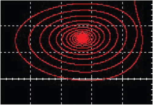
Figure 1. Phase portraits of the chaotic orbit with c=25.
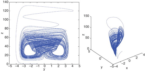
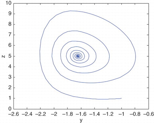
Figure 2. Phase portraits (y−z) of the regular orbit with c=5.
The equilibria as particular solutions of the system meet the following algebraic equations:
3. Distinguishing orbits by different chaotic indicators
There are various methods to distinguish between chaotic and ordered orbits. Now we propose three methods to deal with our problems.
3.1 Lyapunov exponents
In classical physics, LEs, as a common chaos indicator to distinguish whether a system is chaotic or regular, have been widely used to measure the chaoticity of orbits in the nonlinear dynamical system. They calculate the rate of exponential divergence between neighboring trajectories in the phase space, precisely, if the motion is ordered, the corresponding LEs are all negative, otherwise. If the motion is chaotic, the largest LE is strictly positive. There are two different methods for numerically calculating LEs. One rigorous method is to use the tangent vector from the solution of the variational equations of the system. Another less rigorous method is the so-called two-particle method (Tancredi, Sanchez, & Roig, Citation2001) using the deviation vector between two nearby trajectories in place of the tangent vector. All LEs of the three-dimensional system (1) can be attained, where initial conditions are (x, y, z)=(1,−1, 1). In the case c=5, there are three negative LEs (). This sufficiently tests that the system is Lyapunov stable and its attractor is a stable fixed point. For c=25, there are one positive and three negative LEs (
). The onset of such a positive LE confirms that the system is dynamically unstable and chaotic.
An ordered and chaotic behavior can be checked with the LEs method varying system parameters. There is a sudden varying from regular behaviors to chaotic ones when the parameter c passes 7.31 as shown in . In addition, a bifurcation is very convenient to search for an abrupt change of a qualitatively different solution (such as the structure of attractors) for a nonlinear system when a control parameter is smoothly changed. With the help of the bifurcation, a period doubling, quadrupling, etc., and the onset of chaos can be found. Let the parameter c vary in the interval [2.0, 10.0] and give the initial condition (1,−1, 1), the bifurcation diagram versus c is proposed to show how system changes with increasing value of parameter c displayed in . The bifurcation is good to show the transition to chaos as the parameter spans 7.31. The above ways offer enough dynamical information that c=7.31 is a threshold value from regular to chaotic motion.
Figure 3. Lyapunov spectra with the variations of c.
Figure 4. Bifurcation diagrams of max y versus c.
3.2 Fast Lyapunov indicators
It is well known that the time necessary to reach a limit value, either of the length of any tangential vector or of the angle between tangent vectors, is taken as an indicator of stochasticity for a nonlinear dynamical system. Following this general idea, FLI, as a simple, qualitative index, was first introduced by Froeschlé et al. and then modified by Froeschlé and Lega (Citation2000). Given any threshold, the FLI will reach the value fast for a chaotic orbit, and slowly for a regular orbit. Conversely, in the same time span, the indicators will show different values for a regular and a chaotic nature of orbit with completely different time rates. More specifically, the logarithm of the length of a tangent vector method of inspecting the dynamics of a nonlinear physical evolves exponentially for a chaotic orbit, grows only polynomially for a regular motion. In addition, this index was further developed as the two-particle method (Wu& Xie, Citation2007, Citation2008) in which the equations of motion must be solved two times, and the renormalization technique was used to calculate their FLI within a sufficiently long time span. As shown from that FLIs change with the two different values of parameter c. The variations of FLIs are entirely different for the two case. The FLIs are almost invariant for c=5, but some grow exponentially for c=25. As a consequence, the orbit is regular for the former, but chaotic for the latter. The result is consistent with the one given by the the Hopf bifurcation and LEs. It has proved successful that FLI succeeds in detecting the nature of orbits faster than the computation of the LEs due to less or no renormalization.
Figure 5. The FLIs versus log(t).
3.3 Small Alignment index
The construction of SALI (Skokos, Citation2001)also stems from the idea of the calculation of two LEs in any degree system. Two deviation vectors at the same point in the tangent space converge to the direction of the eigenvector which corresponds to the maximal Lyapunov characteristic exponent (LCE) if the Gram–Schmidt orthogonalization is not used. In general, any two randomly chosen initial tangent vectors will become aligned with the most unstable direction and the angle between them will rapidly converge to zero. The speed of the convergence is completely of a opposite nature for chaotic and regular orbits, namely the misalignment between the two tangent vectors tends rapidly to zero for chaotic orbits, while it shows small fluctuations around non-zero values for ordered orbits and so it clearly detects between the two types of orbits. The SALI method has already been confirmed to be an efficient and quick indicator of chaoticity for diagnosing between chaotic and ordered motion independent of the dimensions of the system. In our opinion, the indicator is still suitable for a dissipative system because the speed of the SALI converging to zero is strongly linked to the properties of trajectories but does not at all depend on the conservative or dissipative nature of the system. The SALI also converges exponentially to zero for chaotic orbits in dissipative systems, while it exhibits small fluctuations around non-zero values for ordered ones. These facts can be confirmed in . The SALI grows to a constant for c=5. This is a regular behavior of the orbit. But the case c=25 means the appearance of chaos because their SALIs are fast close to the value −16 before t=10, 000. The result is in conformity to one given by the above other methods.
Figure 6. The SALIs versus log(t).
4. Circuit realization of the chaotic system
There are some common methods of the circuit realization of the chaotic system: one of them is to apply the piece-wise linear function to replace the quadratic, cubic term or other nonlinear term. Other of methods is to use the switch function to substitute the nonlinear term, respectively. The present system is implemented by applying analog multiplier to replace the quadratic product term and by using the triode emitter junction to substitute exponent term, without influencing the system original nonlinear nature. In a practical circuit implementation concerning signals needs to be observed, the strength of the experimental circuit signals is changed to some scale to that of the original circuit signals so that the implementation can be obtained without any difficulty. Of course, the replacement of chaotic variables does not change system properties. As shown in , the voltages C1, C2, and C3 are used as , and
, respectively. The operational amplifiers and its electronic circuitry perform the basic operations of addition, subtraction and integration. In the light of the characters of ideal op-amp (virtual short and virtual open) and the Kirchhoff's current and voltage laws, the corresponding circuit equation can be described as
Figure 7. Circuit diagram of the system.
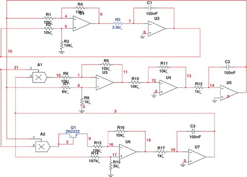
Figure 8. The experiment observations (y−z) of chaotic orbit with c=25.
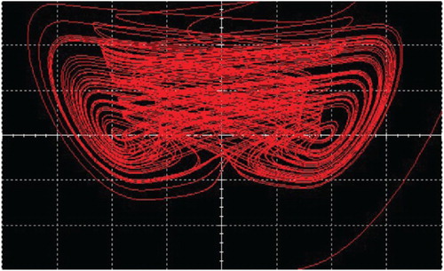
Figure 9. The experiment observations (y−z) of regular trajectory with c=5.
5. Conclusions
A new modified LÜ chaotic system has been investigated with exponential terms. Some basic properties of this system have been discussed in terms of chaotic attractors, equilibria, and eigenvalues of the Jacobian matrices. Bifurcations, LEs are used to find the dependence of the transitivity from order to chaos on changing parameter c. As a result, they get the same results that c=7.31 is a threshold value from a regular dynamic to an irregular one. Namely, under some necessary conditions for the occurrence of chaotic motions, increasing the parameter c always leads to the strength of chaos. With the help of SALIs and FLI, we can explore two different types of orbits (regular or chaotic), as the dynamical parameter c varies. In addition, an electronic circuitry is designed for the realization of the chaotic attractor, identifying experiment results with computer simulations. The new chaotic systems can be regarded as information sources that naturally produce digital communication signals.
REFERENCES
- Arrowsmith, D. K., & Place, C. M. (1990). An introduction to dynamical systems. New York, NY: Cambridge University Press.
- Benettin, G., Galgani, L., & Strelcyn, J.-M. (1976). Kolmogorov entropy and numerical experiments. Physical Review A, 14, 2338–2345. doi: 10.1103/PhysRevA.14.2338
- Cafagna, D., & Grassi, G. (2003). New 3D-scroll attractors in hyperchaotic Chua's circuits forming a ring. International Journal of Bifurcation and Chaos, 13, 2889–2903. doi: 10.1142/S0218127403008284
- Chen, G., & Ueta, T. (1999). Yet another chaotic attractor. International Journal of Bifurcation and Chaos, 9(7), 1465–1466. doi: 10.1142/S0218127499001024
- Contopoulos, G. (2002). Order and chaos in dynamical astronomy. Berlin: Springer Verlag.
- Froeschlé, C., & Lega, E. (2000). On the structure of symplectic mappings. The fast Lyapunov indicator: A very sensitive tool. Celestial Mechanics and Dynamical Astronomy, 78, 167–195.
- Froeschlé, C., Lega, E., & Gonczi, R. (1997). Fast Lyapunov indicators. Applications to asteroidal motion. Celestial Mechanics and Dynamical Astronomy, 67, 41–62. doi: 10.1023/A:1008276418601
- Hénon, M., & Heils, C. (1964). The applicability of the third integral of motions: Some numerical experiments. Astronomical Journal, 69, 73–79. doi: 10.1086/109234
- Huang, G.-Q., & Wu, X. (2012). Analysis of new four-dimensional chaotic circuits with experimental and numerical methods. International Journal of Bifurcation and Chaos, 22(2), 1250042 (13 pp.). doi: 10.1142/S0218127412500423
- Lorenz, E. N. (1963). Deterministic nonperiodic flow. Journal of Atmospheric Sciences, 20, 130–141. doi: 10.1175/1520-0469(1963)020<0130:DNF>2.0.CO;2
- Lü, J., & Chen, G. (2002). A new chaotic attractor coined. International Journal of Bifurcation and Chaos, 12(3), 659–661. doi: 10.1142/S0218127402004620
- Matsumoto, T., Chua, L. O., & Kobayashi, K. (1986). Hyperchaos: Laboratory experiment and numerical confirmation. IEEE Transactions on Circuits and Systems, 33, 1143–1147. doi: 10.1109/TCS.1986.1085862
- Qi, G. Y., Wyk, M. A., Wyk, B. J., & Chen, G. R. (2009). A new hyperchaotic system and its circuit implementation. Chaos, Solitons and Fractals, 40, 2544–2549. doi: 10.1016/j.chaos.2007.10.053
- Rössler, O. E. (1979). An equation for hyperchaos. Physics Letters A, 71(2,3), 155–156. doi: 10.1016/0375-9601(79)90150-6
- Skokos, C. (2001). Alignment indices: A new, simple method for determining the ordered or chaotic nature of orbits. Journal of Physics A, 34, 10029–10043. doi: 10.1088/0305-4470/34/47/309
- Skokos, Ch., Bountis, T., & Antonopoulos, Ch. (2007). Geometrical properties of local dynamics in Hamiltonian systems: The Generalized Alignment Index (GALI) method. Physica D, 231, 30–54. doi: 10.1016/j.physd.2007.04.004
- Tancredi, G., Sanchez, A., & Roig, F. (2001). A comparison between methods to compute Lyapunov exponents. Astronomical Journal, 121, 1171–1179. doi: 10.1086/318732
- Wu, X., & Xie, Y. (2007). Revisit on “Ruling out chaos in compact binary systems”. Physical Review D, 76(6), 124004D. doi: 10.1103/PhysRevD.76.124004
- Wu, X., & Xie, Y. (2008). Resurvey of order and chaos in spinning compact binaries. Physical Review D, 77(10), 103012. doi: 10.1103/PhysRevD.77.103012