Energy-based Hamiltonian approach in H_∞ controller design for n-degree of freedom mechanical systems

Abstract

This paper studies the energy-based approach for $H_{\mathrm{\infty }}$ controller design of $n$-degree of freedom mechanical systems. In this approach, the Hamiltonian function, which is the sum of kinetic and potential energies of the system, is considered as the Lyapunov function for stability analysis. The stability analysis is done based on the port-controlled Hamiltonian (PCH) model. In this regard, two theorems are given and proved that the proposed controllers lead to $H_{\mathrm{\infty }}$ disturbance attenuation for both absolutely known system model and unknown ones with parametric uncertainties. In the case of parametric uncertainties, the energy-based controller has an adaptive approach. Performance of proposed controllers is illustrated through simulations taken on a 2-link robot manipulator system, which validate the theoretical achievements of this paper.

KEYWORDS:

• Energy-based control
• $H_{\mathrm{\infty }}$ controller
• mechanical system
• port-controlled Hamiltonian (PCH)
• external disturbances
• parametric uncertainty
• adaptive control

1. Introduction

Control of mechanical systems has been an important topic that attracts the attention of researchers due to their vast application areas, such as industrial, medical, space and marine (Shafiei & Binazadeh, 2014, 2015). Mechanical systems require high precision control in order to achieve their desired performance (Hakimi & Binazadeh, 2017). Even though, several items cause a complicated controller design procedure, including the nonlinear dynamic feature of mechanical systems, unavoidable risk of being exposed to external disturbances and parametric uncertainties, which stem from environmental factors and system identification failures.

Different robust methods have been proposed in Literature (Wang, Yang, & Yan, 2019; Wu & Lu, 2018; Wu, Lu, Shi, Su, & Wu, 2018). Among them, the $H_{\mathrm{\infty }}$ controller is not only known in attenuating the effects of matched and unmatched disturbances, but it also is capable to attenuate the impacts of model uncertainties (Acho, Orlov, & Solis, 2001; Erol & Delibaşı, 2018; Orlov & Aguilar, 2014; van der Schaft, 2001). While, general solutions have been presented for $H_{\mathrm{\infty }}$ controllers (Gholami & Binazadeh, 2019a, 2019b; Li & Liao, 2018; Orlov & Aguilar, 2014; van der Schaft, 2001), the major drawback is the difficulty of solving HJI inequalities where in the design procedure leads to an infinite dimension problem (Krstic & Deng, 1998; Subbotin, 1995). This fact causes local solutions for many problems (Orlov & Aguilar, 2004). While global stability has been proved by means of other control methods (Chung, Fu, & Hsu, 2008; Kelly, Santibanez, & Loria, 2005).

Mechanical systems are highly nonlinear systems which are dynamically coupled (Binazadeh & Shafiei, 2016). Some parameter approximations in the modelling of these systems result in parametric uncertainty. Furthermore, some dynamics of the system may not be considered due to model simplification. In addition, the effect of external disturbances on mechanical systems is unavoidable. Authors of (Chavez Guzmán, Aguilar Bustos, & Mérida Rubio, 2015) have designed adaptive $H_{\mathrm{\infty }}$ controller for $n$-degree of freedom robot manipulator system in spite of external disturbances. This goal is achieved by exploiting compensators or pre-compensators of gravitational forces. Furthermore, the design of adaptive tracking $H_{\mathrm{\infty }}$ controller for the mobile robot has been studied in (Sato, Yanagi, & Tsuruta, 2011) based on inverse optimal control strategy.

One of the important approaches in controller design for mechanical systems is energy-based control (Valentinis, Donaire, & Perez, 2015; Yang & Xian, 2019). Energy-based control laws are based on the stored energy in the system. The stored energy acts as the Lyapunov function and the nonlinear control methods which are based on the Lyapunov function may be applied in the energy-based control.

The essential step in exploiting the energy-based Hamiltonian approach is to transform the system into a PCH model. This issue firstly was introduced in (Maschke & Schaft, 1992). Generally, this technique uses properties of the internal structure of the actual system in designing controllers and gives a relatively simpler controller with better performance.

In this regard, this paper considers the design of $H_{\mathrm{\infty }}$ controller based on the energy concept for $n$-degree of freedom mechanical systems to attenuate the effects of external disturbances and parametric uncertainties via an adaptive approach. The equations of the foresaid systems are considered in two cases. First, all parameters of the system are assumed to be known. In the second case, parametric uncertainties are considered in the system model. In both, disturbance inputs with bounded energies are considered. As the first step, system equations are transformed into PCH structure. Then, by utilizing the energy concept, $H_{\mathrm{\infty }}$ controllers are designed. The key contributions of this paper are summarized below.

• This paper studies the energy-based $H_{\mathrm{\infty }}$ control design for disturbance attenuation which is applicable to a broad class of mechanical systems.

• The proposed approach has also a robust manner in the face of parametric uncertainties.

• The adaptive control is combined with the energy-based control to improve the robust performance in the presence of parametric uncertainties.

• The proposed approach leads to relatively simpler controllers with better performance over the other robust control strategies.

Furthermore, the validity of the proposed approach is verified by using the simulation of a 2-link robot manipulator system.

2. Preliminaries

In this section, some necessary definitions are briefly reviewed.

Definition 2.1

PCH system

(Ortega, van der Schaft, Maschke, & Escobar, 2002): If dynamic equations of a system could be written in the following structure, then it is called a PCH system: (1) $\left\{\begin{array}{l}\dot{x}=\left[J\left(x\right)-R\left(x\right)\right]\frac{\mathrm{\partial }H\left(x\right)}{\mathrm{\partial }x}+g\left(x\right)u\\ y=g^T\left(x\right)\frac{\mathrm{\partial }H\left(x\right)}{\mathrm{\partial }x}\end{array}\right.$(1) where $x=[x_1,\cdots ,x_n{]}^T$ is the state vector of the system and $J\left(x\right)$ is a skew-symmetric matrix ($J\left(x\right)=-J^T\left(x\right)$), called the interconnection matrix. Moreover, $H\left(x\right)$ is the Hamiltonian function which is the sum of kinetic and potential energies of the system, $R\left(x\right)$ is a symmetric matrix known as damping matrix and $g\left(x\right)$ is the input matrix. One of the main benefits of the PCH system is that its Hamiltonian function $H\left(x\right)$ can be used as the Lyapunov function for the stability analysis of the systems.

Definition 2.2

Finite-gain ${\mathcal{L}}_p$ stability

(Khalil, 2014): A dynamic system with the input signal $u$ and the output signal $y$ is ${\mathcal{L}}_p$ stable with a finite-gain, if there exist a positive constant $\gamma$ and a nonnegative constant $\beta$ such that the following inequality holds: (2) $||y|{|}_{{\mathcal{L}}_p}\le \gamma ||u|{|}_{{\mathcal{L}}_p}+\beta$(2) the constant $\gamma$ is the ${\mathcal{L}}_p$ gain and $||y\left(t\right)|{|}_{{\mathcal{L}}_p}={\left({\int }_0^{\mathrm{\infty }}||y\left(t\right)|{|}_p^p\right)}^{\frac{\text{1}}{p}},||y\left(t\right)|{|}_p^p=\sum _i{|y_i|}^p$ where $y_i$ is the ith component of vector $y$. For $p=2$, the above inequality represents the ${\mathcal{L}}_2$ stability between the input $u$ and the output $y$ of the dynamical system and, $\gamma$ is called the ${\mathcal{L}}_2$ gain of the system.

3. Problem statement

In general, the motion equation of $n$-degree of freedom mechanical systems is considered as below (Ortega, Loria, Nicklasson, & Sira-Ramirez, 1998): (3) $M\left(q\right)\ddot{q}+C\left(q,\dot{q}\right)\dot{q}+B\left(q\right)=G\left(q\right)u$(3) in which $q\left(t\right)=[q_1,q_2,\dots ,q_n{]}^T\in {\mathbb{R}}^n$ is the position vector, $\dot{q}\in {\mathbb{R}}^n$ is the velocity vector, $M\left(q\right)=M^T\left(q\right)>0\in {\mathbb{R}}^{n\times m}$ is the inertia matrix, $C\left(q,\dot{q}\right)$ is the coriolis and centripental forces vector, $B\left(q\right)\in {\mathbb{R}}^n$ is the potential forces vector, $G\left(q\right)\in {\mathbb{R}}^{n\times m}$ is the input coupling matrix and $u\in {\mathbb{R}}^m$ is the applied torque vector.

In fact, there exist a variety of systems with the structure of Equation (3) such as quadrotor (Zheng, Zhu, Zuo, & Yan, 2015), wheeled inverted pendulum (Delgado & Kotyczka, 2016) and many other mechanical systems.

In the presence of the time-varying external disturbances $\delta \left(t\right)$, the dynamical Equations (3) can be written as (4) $M\left(q\right)\ddot{q}+C\left(q,\dot{q}\right)\dot{q}+B\left(q\right)=G\left(q\right)u+\delta \left(t\right)$(4) In this paper, the goal is to design an appropriate control law such that $q$ and $\dot{q}$ converge to the desired values in spite of unknown energy-bounded disturbances. A tool to achieve this, is using the energy-based Hamiltonian concept. In this regard, it is necessary to transform the dynamical Equations (3) into the PCH structure, firstly.

4. Construction of PCH form for the nominal system

In this section, it is aimed to transform the nominal system (3) into the PCH form. The Hamiltonian function of the system (3) is (5) $H\left(q,p\right)=K\left(q,p\right)+V_0\left(q\right)$(5) where $p\in {\mathbb{R}}^n$ is the inertia vector of the system and $M^{-1}\left(q\right)p=\dot{q}$. Moreover, $K\left(q,p\right)$ and $V_0\left(q\right)$ are kinetic and potential energies of the system, respectively and (6) $\begin{array}{rl}K\left(q,p\right)& =\frac{\text{1}}{\text{2}}{p}^T{M}^{-1}\left(q\right)p\\ & =\frac{\text{1}}{\text{2}}{\dot{q}}^{T}M\left(q\right)\dot{q}\end{array}$(6) (7) $\begin{array}{rl}{V}_0\left(q\right)& =\int B\left(q\right)dq\end{array}$(7) where $M\left(q\right)$ and $B\left(q\right)$ are introduced in (3).

The following lemma is employed in the procedure of constructing the PCH form.

Lemma 4.1

Wang & Ge, 2008

Assume that $A\left(x\right)\in {\mathbb{R}}^{n\times n}\left(x\in {\mathbb{R}}^n\right)$ is a matrix function and $\alpha \mathrm{\&}\beta \in {\mathbb{R}}^n$ are constant vectors, then: (8) $\frac{\mathrm{\partial }\left({\alpha }^{T}A\left(x\right)\beta \right)}{\mathrm{\partial }x}=\left(I_n\otimes {\alpha }^T\right)\left({\mathrm{\Gamma }}_n\frac{\mathrm{\partial }A\left(x\right)}{\mathrm{\partial }x}\right)\beta$(8) in which $\frac{\mathrm{\partial }A\left(x\right)}{\mathrm{\partial }x}=A\left(x\right)\otimes \frac{\mathrm{\partial }}{\mathrm{\partial }x}$ and ${\mathrm{\Gamma }}_n$ is defined as (9) $\begin{array}{rl}{\mathrm{\Gamma }}_n& =\prod _{i=\text{1}}^{n-\text{1}}\prod _{j>i}^n{E}_{n^{\text{2}}}\left(\left(i-\text{1}\right)n+j,\left(j-\text{1}\right)n+i\right);\\ & E_{n^{\text{2}}}\left(\left(i-\text{1}\right)n+j,\left(j-\text{1}\right)n+i\right)\in {\mathbb{R}}^{n^{\text{2}}\times n^{\text{2}}}\end{array}$(9) where $E_n\left(i,j\right)\in {\mathbb{R}}^{n\times n}$ is the so-called row-swap matrix operator and is obtained by swapping the $i$th row with the $j$th row of the identity matrix $I_{n\times n}$.

Based on Lemma 4.1, the following equation is obtained: (10) $\frac{\mathrm{\partial }H\left(q,p\right)}{\mathrm{\partial }q}=\frac{\text{1}}{\text{2}}\left(I_n\otimes p^T\right)\left({\mathrm{\Gamma }}_n\frac{\mathrm{\partial }{M}^{-\text{1}}}{\mathrm{\partial }q}\right)p+\frac{\mathrm{\partial }{V}_{\text{0}}\left(q\right)}{\mathrm{\partial }q}$(10) Furthermore, taking the derivative of the Hamiltonian function with respect to $p$ and considering $p=M\left(q\right)\dot{q}$, one has (11) $\begin{array}{rl}\frac{\mathrm{\partial }H\left(q,p\right)}{\mathrm{\partial }p}& =M^{-\text{1}}\left(q\right)p\\ & =\dot{q}\end{array}$(11)

It is concluded that: (12) $p=M\left(q\right)\dot{q}$(12) Taking the time derivative of (12) and considering the nominal system (3) gives the following equation: (13) $\begin{array}{rl}\dot{p}& =\dot{M}\left(q\right)\dot{q}+M\left(q\right)\ddot{q}\\ & =\dot{M}\left(q\right)\dot{q}-C\left(q,\dot{q}\right)\dot{q}-B\left(q\right)+G\left(q\right)u\left(t\right)\\ & =\left(\dot{M}\left(q\right)-C\left(q,\dot{q}\right)\right)\dot{q}-B\left(q\right)+G\left(q\right)u\left(t\right)\end{array}$(13) according to (7), $V_{\text{0}}\left(q\right)=\int B\left(q\right)dq\Rightarrow B\left(q\right)=\frac{\mathrm{\partial }{V}_{\text{0}}}{\mathrm{\partial }q}$. Replacing this relation in (13) results in: (14) $\dot{p}=\left(\dot{M}\left(q\right)-C\left(q,\dot{q}\right)\right)\dot{q}-\frac{\mathrm{\partial }{V}_{\text{0}}}{\mathrm{\partial }q}+G\left(q\right)u\left(t\right)$(14) with regard to (10), (11), the above relation can be rewritten as bellow (15) $\dot{p}=-\frac{\mathrm{\partial }H\left(q,p\right)}{\mathrm{\partial }q}+K_C\left(q,p\right)\frac{\mathrm{\partial }H\left(q,p\right)}{\mathrm{\partial }p}+G\left(q\right)u\left(t\right)$(15) where (16) $K_C\left(q,p\right)=\dot{M}\left(q\right)-C\left(q,\dot{q}\right)+\frac{\text{1}}{\text{2}}\left(I_n\otimes p^T\right)\left({\mathrm{\Gamma }}_n\frac{\mathrm{\partial }{M}^{-\text{1}}}{\mathrm{\partial }q}\right)M\left(q\right)$(16) Considering (11) and (15), one may write: (17) $\left[\begin{array}{c}\dot{q}\\ \dot{p}\end{array}\right]=\left[\begin{array}{cc}\text{0}& I_n\\ -I_n& K_C\left(q,p\right)\end{array}\right]\left[\begin{array}{c}\frac{\mathrm{\partial }H\left(q,p\right)}{\mathrm{\partial }q}\\ \frac{\mathrm{\partial }H\left(q,p\right)}{\mathrm{\partial }p}\end{array}\right]+\left[\begin{array}{c}\text{0}\\ G\left(q\right)\end{array}\right]u$(17) by using properties of Kronecker product it is proved that $K_C\left(q,p\right)\equiv 0$ (the details is given by Wang and Ge (2008))

If we define: (18) $x=\left[\begin{array}{c}q\\ p\end{array}\right]$(18) then, relation (17) has the PCH form as follows: (19) $\dot{x}=\left[J\left(x\right)-R\left(x\right)\right]\frac{\mathrm{\partial }H\left(x\right)}{\mathrm{\partial }x}+g_{c}u$(19) where $\begin{array}{rl}J\left(x\right)& =\left[\begin{array}{cc}0& I_n\\ -I_n& 0\end{array}\right]\\ R\left(x\right)& =\left[\begin{array}{cc}0& 0\\ 0& 0\end{array}\right]\\ \frac{\mathrm{\partial }H\left(x\right)}{\mathrm{\partial }x}& =\left[\begin{array}{c}\frac{\mathrm{\partial }H\left(q,p\right)}{\mathrm{\partial }q}\\ \frac{\mathrm{\partial }H\left(q,p\right)}{\mathrm{\partial }p}\end{array}\right]\\ g_c& =\left[\begin{array}{c}0\\ G\left(q\right)\end{array}\right]\end{array}$it is obvious that $J\left(x\right)=-J^T\left(x\right)$ and $R\left(x\right)=R^T\left(x\right)\ge 0$.

5. Design of nonlinear $H_{\mathrm{\infty }}$ controller for the nominal system

In this section, by using the PCH structure obtained in the previous section, an energy-based $H_{\mathrm{\infty }}$ controller is designed to attenuate the impact of disturbances on the output of the system. In other word, a control law is designed such that, if $\delta$ be an unknown disturbance input with finite ${\mathcal{L}}_2$ norm, then ${\mathcal{L}}_2$ norm of the output $y$ stays bounded and there exists an attenuation ratio $\gamma >0$ between ${\mathcal{L}}_2$ norm of the disturbance input and output (refer to Definition 2.2). In this regard the following assumption is given:

Assumption 5.1:

The external time-varying disturbance vector $\delta \left(t\right)$ belongs to ${\mathcal{L}}_2$ space. It means that $||\delta |{|}_{{\mathcal{L}}_{\text{2}}}=\sqrt{{\int }_{\text{2}}^{\mathrm{\infty }}{\delta }^T\text{(}t\text{)}\delta \text{(}t\text{)}dt}\le \eta ,\eta >\text{0}$

This is a common assumption for $H_{\mathrm{\infty }}$ disturbance attenuation in the dynamical systems which states the external disturbance vector is energy bounded for all $t\in \left[0,\mathrm{\infty }\right)$.

By considering the output of the system as (20) $y=h\left(x\right)g_c^T\left(x\right)\frac{\mathrm{\partial }H\left(x\right)}{\mathrm{\partial }x}$(20) where $y\in {\mathbb{R}}^q$ and $h\left(x\right)\in {\mathbb{R}}^{q\times m}$ is a weighting matrix with full coloumn rank, then according to the PCH structure of the system (3), equations of system (4) can be written in the following PCH form: (21) $\left\{\begin{array}{l}\dot{x}=\left[J\left(x\right)-R\left(x\right)\right]\frac{\mathrm{\partial }H\left(x\right)}{\mathrm{\partial }x}+g_{c}u+g_d\delta \\ y=h\left(x\right)g_c^T\left(x\right)\frac{\mathrm{\partial }H\left(x\right)}{\mathrm{\partial }x}\end{array}\right.$(21) where $g_d=[0I_n{]}^T$ and $R\left(x\right)=0$.

Definition 5.1

Asadinia & Binazadeh, 20192019

The dynamical system (21) is supposed to have $H_{\mathrm{\infty }}$ disturbance attenuation property if the following condition holds for a positive constant $\gamma$, (22) ${\int }_0^{\mathrm{\infty }}{y}^T\left(t\right)y\left(t\right)dt\le {\gamma }^2{\int }_0^{\mathrm{\infty }}{\delta }^T\left(t\right)\delta \left(t\right)dt$(22) where $||y\left(t\right)|{|}_2^2=y(t{)}^{T}y\left(t\right)$ and in what follows the notation $||.||=||.|{|}_2$ is assumed. The above relation is also called as $H_{\mathrm{\infty }}$ performance index. The task is the design of control law $u\left(t\right)$ for the system (21) such that the $H_{\mathrm{\infty }}$ disturbance attenuation property is satisfied for the closed-loop system. In this regard, the following theorem is given and proved.

Theorem 5.1:

For a defined disturbance attenuation ratio $\gamma >0$, if the following inequality holds: (23) $\left[\begin{array}{cc}\text{0}& \text{0}\\ \text{0}& K_u\end{array}\right]-\frac{\text{1}}{\text{2}{\gamma }^{\text{2}}}{g}_d{g}_d^T\ge \text{0}$(23) in which $K_u\in {\mathbb{R}}^{n\times n}$ is a positive-definite matrix, then if $G$ be invertible the following control law satisfies the $H_{\mathrm{\infty }}$ performance index for the system (21): (24) $u=-\frac{\text{1}}{\text{2}}\left(g_c^{†}Q+h{\left(x\right)}^{T}h\left(x\right)g_c^T\right)\frac{\mathrm{\partial }H\left(x\right)}{\mathrm{\partial }x}-G^{-\text{1}}{K}_u\dot{q}$(24) where $Q$ is a positive-definite matrix. Moreover, $g_c^{†}$ is the pseudo-inverse of $g_c$.

Proof:

Substituting control law (24) into the system Equations (21) and taking into account that $g_c{G}^{-1}\left(q\right)=\left[\begin{array}{c}{0}_{n\times n}\\ G\left(q\right)\end{array}\right]G^{-1}\left(q\right)=\left[\begin{array}{c}{0}_{n\times n}\\ I_{n\times n}\end{array}\right]$, the closed-loop system equations become: (25) $\left\{\begin{array}{l}\dot{x}=J\left(x\right)\frac{\mathrm{\partial }H\left(x\right)}{\mathrm{\partial }x}-\frac{\text{1}}{\text{2}}\left(Q+g_{c}h{\left(x\right)}^{T}h\left(x\right)g_c^T\right)\frac{\mathrm{\partial }H\left(x\right)}{\mathrm{\partial }x}\\ +\left[\begin{array}{c}\text{0}\\ -K_u\dot{q}\end{array}\right]+g_d\delta \\ y=h\left(x\right)g_c^T\left(x\right)\frac{\mathrm{\partial }H\left(x\right)}{\mathrm{\partial }x}\end{array}\right.$(25) furthermore, since $\dot{q}=\frac{\mathrm{\partial }H\left(x\right)}{\mathrm{\partial }p}$ it is concluded that $\begin{array}{rl}\left[\begin{array}{c}0\\ -K_u\dot{q}\end{array}\right]& =-\left[\begin{array}{cc}0& 0\\ 0& K_u\end{array}\right]\frac{\mathrm{\partial }H\left(x\right)}{\mathrm{\partial }x}=-\left[\begin{array}{cc}0& 0\\ 0& K_u\end{array}\right]\\ & \times \left[\begin{array}{c}\frac{\mathrm{\partial }H\left(x\right)}{\mathrm{\partial }q}\\ \frac{\mathrm{\partial }H\left(x\right)}{\mathrm{\partial }p}\end{array}\right]\end{array}$Thus: (26) $\begin{array}{rl}\dot{x}& =J\left(x\right)\frac{\mathrm{\partial }H\left(x\right)}{\mathrm{\partial }x}-\frac{1}{2}\left(Q+g_{c}h{\left(x\right)}^{T}h\left(x\right)g_c^T\right)\frac{\mathrm{\partial }H\left(x\right)}{\mathrm{\partial }x}\\ & -\left[\begin{array}{cc}0& 0\\ 0& K_u\end{array}\right]\frac{\mathrm{\partial }H\left(x\right)}{\mathrm{\partial }x}+g_d\delta \end{array}$(26) Considering the Hamiltonian function as the Lyapunov function candidate and taking its derivative along the trajectories of the closed-loop system (26), results in: (27) $\begin{array}{rl}\dot{H}\left(x\right)& =\frac{{\mathrm{\partial }}^{T}H\left(x\right)}{\mathrm{\partial }x}\dot{x}\\ & =\frac{{\mathrm{\partial }}^{T}H\left(x\right)}{\mathrm{\partial }x}J\left(x\right)\frac{\mathrm{\partial }H\left(x\right)}{\mathrm{\partial }x}+\frac{{\mathrm{\partial }}^{T}H\left(x\right)}{\mathrm{\partial }x}\\ & \times \left(-\frac{\text{1}}{\text{2}}\left(Q+g_{c}h{\left(x\right)}^{T}h\left(x\right)g_c^T\right)\right.\left.-\left[\begin{array}{cc}\text{0}& \text{0}\\ \text{0}& K_u\end{array}\right]\right)\frac{\mathrm{\partial }H\left(x\right)}{\mathrm{\partial }x}\\ & +\frac{{\mathrm{\partial }}^{T}H\left(x\right)}{\mathrm{\partial }x}{g}_d\delta \end{array}$(27) whereas $J\left(x\right)$ is a skew-symmetric matrix ($J\left(x\right)=-J^T\left(x\right)$), then $\frac{{\mathrm{\partial }}^{T}H\left(x\right)}{\mathrm{\partial }x}J\left(x\right)\frac{\mathrm{\partial }H\left(x\right)}{\mathrm{\partial }x}=0$. Therefore, (28) $\begin{array}{rl}\dot{H}\left(x\right)& =\frac{{\mathrm{\partial }}^{T}H\left(x\right)}{\mathrm{\partial }x}\left(-\frac{\text{1}}{\text{2}}\left(Q+g_{c}h{\left(x\right)}^{T}h\left(x\right)g_c^T\right)\right.\left.-\left[\begin{array}{cc}\text{0}& \text{0}\\ \text{0}& K_u\end{array}\right]\right)\\ & \times \frac{\mathrm{\partial }H\left(x\right)}{\mathrm{\partial }x}+\frac{{\mathrm{\partial }}^{T}H\left(x\right)}{\mathrm{\partial }x}{g}_d\delta \end{array}$(28) as $Q$ is assumed to be positive-definite, $\left(-\frac{\text{1}}{\text{2}}\frac{{\mathrm{\partial }}^{T}H\left(x\right)}{\mathrm{\partial }x}Q\frac{\mathrm{\partial }H\left(x\right)}{\mathrm{\partial }x}\right)\le \text{0}$ and Equation (28) leads to the following inequality: (29) $\begin{array}{rl}\dot{H}\left(x\right)\le & -\frac{\text{1}}{\text{2}}\frac{{\mathrm{\partial }}^{T}H\left(x\right)}{\mathrm{\partial }x}{g}_{c}h(x{)}^{T}h\left(x\right)g_c^T\frac{\mathrm{\partial }H\left(x\right)}{\mathrm{\partial }x}\\ & -\frac{{\mathrm{\partial }}^{T}H\left(x\right)}{\mathrm{\partial }x}\left[\begin{array}{cc}\text{0}& \text{0}\\ \text{0}& K_u\end{array}\right]\frac{\mathrm{\partial }H\left(x\right)}{\mathrm{\partial }x}+\frac{{\mathrm{\partial }}^{T}H\left(x\right)}{\mathrm{\partial }x}{g}_d\delta \end{array}$(29) According to the predefined output for the system (25), the relation (29) can be rewritten as (30) $\begin{array}{rl}\dot{H}\left(x\right)\le & -\frac{\text{1}}{\text{2}}{y}^T\text{y}\\ & -\frac{{\mathrm{\partial }}^{T}H\left(x\right)}{\mathrm{\partial }x}\left[\begin{array}{cc}\text{0}& \text{0}\\ \text{0}& K_u\end{array}\right]\frac{\mathrm{\partial }H\left(x\right)}{\mathrm{\partial }x}+\frac{{\mathrm{\partial }}^{T}H\left(x\right)}{\mathrm{\partial }x}{g}_d\delta \end{array}$(30) Considering that $y^T\text{y}=||y|{|}^2$ and by adding and subtracting $\frac{1}{2{\gamma }^2}\frac{{\mathrm{\partial }}^{T}H\left(x\right)}{\mathrm{\partial }x}{g}_d{g}_d^T\frac{\mathrm{\partial }H\left(x\right)}{\mathrm{\partial }x}$ and $\frac{{\gamma }^2}{2}||\delta |{|}^2$ to the right-hand side of (30), one gets (31) $\begin{array}{rl}\dot{H}\left(x\right)\le & -\frac{\text{1}}{\text{2}}||y|{|}^2-\frac{{\mathrm{\partial }}^{T}H\left(x\right)}{\mathrm{\partial }x}\left[\begin{array}{cc}\text{0}& \text{0}\\ \text{0}& K_u\end{array}\right]\frac{\mathrm{\partial }H\left(x\right)}{\mathrm{\partial }x}+\frac{{\mathrm{\partial }}^{T}H\left(x\right)}{\mathrm{\partial }x}{g}_d\delta \\ & +\left(\frac{\text{1}}{\text{2}{\gamma }^{\text{2}}}\frac{{\mathrm{\partial }}^{T}H\left(x\right)}{\mathrm{\partial }x}{g}_d{g}_d^T\frac{\mathrm{\partial }H\left(x\right)}{\mathrm{\partial }x}\right.\\ & -\frac{\text{1}}{\text{2}{\gamma }^{\text{2}}}\frac{{\mathrm{\partial }}^{T}H\left(x\right)}{\mathrm{\partial }x}{g}_d{g}_d^T\left.\frac{\mathrm{\partial }H\left(x\right)}{\mathrm{\partial }x}\right)\\ & +\left(\frac{{\gamma }^2}{\text{2}}{||\delta ||}^{\text{2}}-\frac{{\gamma }^{\text{2}}}{\text{2}}{||\delta ||}^{\text{2}}\right)\end{array}$(31) The right-hand side expressions of inequality (31) can be grouped as (32) $\begin{array}{rl}\dot{H}\left(x\right)\le & -\frac{{\mathrm{\partial }}^{T}H\left(x\right)}{\mathrm{\partial }x}\left[\begin{array}{cc}0& 0\\ 0& K_u\end{array}\right]\frac{\mathrm{\partial }H\left(x\right)}{\mathrm{\partial }x}\\ & +\frac{1}{2{\gamma }^2}\frac{{\mathrm{\partial }}^{T}H\left(x\right)}{\mathrm{\partial }x}{g}_d{g}_d^T\frac{\mathrm{\partial }H\left(x\right)}{\mathrm{\partial }x}\\ & -\left(\frac{1}{2{\gamma }^2}\frac{{\mathrm{\partial }}^{T}H\left(x\right)}{\mathrm{\partial }x}{g}_d{g}_d^T\frac{\mathrm{\partial }H\left(x\right)}{\mathrm{\partial }x}+\frac{{\gamma }^2}{2}{||\delta ||}^2\right.\\ & \left.-\frac{{\mathrm{\partial }}^{T}H\left(x\right)}{\mathrm{\partial }x}{g}_d\delta \right)\\ & +\left(\frac{{\gamma }^2}{2}{||\delta ||}^2-\frac{1}{2}{||y||}^2\right)\end{array}$(32) On the other hand, one has (33) $\begin{array}{rl}\frac{1}{2}{\left|\left|\gamma \delta -\frac{1}{\gamma }{g}_d^T\frac{\mathrm{\partial }H\left(x\right)}{\mathrm{\partial }x}\right|\right|}^2& =\frac{1}{2}{\left(\gamma \delta -\frac{1}{\gamma }{g}_d^T\frac{\mathrm{\partial }H\left(x\right)}{\mathrm{\partial }x}\right)}^T\\ & \times \left(\gamma \delta -\frac{1}{\gamma }{g}_d^T\frac{\mathrm{\partial }H\left(x\right)}{\mathrm{\partial }x}\right)\\ & =\frac{1}{2{\gamma }^2}\frac{{\mathrm{\partial }}^{T}H\left(x\right)}{\mathrm{\partial }x}{g}_d{g}_d^T\frac{\mathrm{\partial }H\left(x\right)}{\mathrm{\partial }x}\\ & +\frac{{\gamma }^2}{2}||\delta |{|}^2-\frac{{\mathrm{\partial }}^{T}H\left(x\right)}{\mathrm{\partial }x}{g}_d\delta \end{array}$(33) Considering (32) and (33), one may write: (34) $\begin{array}{rl}\dot{H}\left(x\right)& \le -\frac{{\mathrm{\partial }}^{T}H\left(x\right)}{\mathrm{\partial }x}\left[\left[\begin{array}{cc}\text{0}& \text{0}\\ \text{0}& K_u\end{array}\right]-\frac{1}{2{\gamma }^2}{g}_d{g}_d^T\right]\frac{\mathrm{\partial }H\left(x\right)}{\mathrm{\partial }x}\\ & -\frac{\text{1}}{\text{2}}{\left|\left|\gamma \delta -\frac{1}{\gamma }{g}_d^T\frac{\mathrm{\partial }H\left(x\right)}{\mathrm{\partial }x}\right|\right|}^2+\frac{\text{1}}{\text{2}}\left({\gamma }^2{||\delta ||}^2-{||y||}^2\right)\end{array}$(34) According to (23), the relation $\left(\frac{{\mathrm{\partial }}^{T}H\left(x\right)}{\mathrm{\partial }x}\left[\left[\begin{array}{cc}\text{0}& \text{0}\\ \text{0}& K_u\end{array}\right]-\frac{1}{2{\gamma }^2}{g}_d{g}_d^T\right]\frac{\mathrm{\partial }H\left(x\right)}{\mathrm{\partial }x}\right)\ge 0$ holds. Since the first and the second expressions of the right-hand side of inequality (34) is non-positive, thus: (35) $\dot{H}\left(x\right)\le \frac{1}{2}\left({\gamma }^2{||\delta ||}^2-{||y||}^2\right)$(35) Taking an integral on inequality (34) over the time-interval $\left[0,\mathrm{\infty }\right)$ leads to: (36) $\begin{array}{rl}& H\left(x\left(\mathrm{\infty }\right)\right)-H\left(x\left(0\right)\right)\\ & \le \frac{\text{1}}{\text{2}}\left({\gamma }^2{\int }_0^{\mathrm{\infty }}{||\delta \left(t\right)||}^{2}dt-{\int }_0^{\mathrm{\infty }}{||y\left(t\right)||}^{2}dt\right)\end{array}$(36) Since $H\left(x\right)$ is a positive function and by assuming $H\left(x\left(0\right)\right)=0$, the following inequality is obtained: (37) $\begin{array}{rl}\text{0}& \le \frac{\text{1}}{\text{2}}\left({\gamma }^2{\int }_0^{\mathrm{\infty }}{||\delta ||}^{2}dt-{\int }_0^{\mathrm{\infty }}{||y||}^{2}dt\right)\\ & \Rightarrow {\int }_0^{\mathrm{\infty }}||y\left(t\right)|{|}^{2}dt\le {\gamma }^2{\int }_0^{\mathrm{\infty }}||\delta \left(t\right)|{|}^{2}dt\end{array}$(37) Therefore, the $H_{\mathrm{\infty }}$ performance index (22) is satisfied for the closed-loop system. This completes the proof.

Remark 5.1:

The convergence speed of the proposed control algorithm can be controlled by appropriate selection of the design matrices $Q$ and $K_u$.

In what follows, the designed controller (24) is applied to a practical system and the simulation results are presented.

6. Design of nonlinear $H_{\mathrm{\infty }}$ controller for 2-link robot manipulator

In this section, the effective performance of the proposed controller is evaluated by applying on a 2-link robot manipulator. The schematic of this system is shown in Figure 1.

Figure 1. 2-link robot manipulator system.

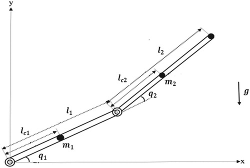
Considering (4), $q=[q_1,q_2{]}^T\in {\mathbb{R}}^2$ is the vector of angular positions which are shown in Figure 1. $u=\tau$ is the control torque and $\delta$ is the external disturbance. Furtheremore, other parameteres of system motion equation is given as bellow (see Ge and Harris (1998) for more details): (38) $\begin{array}{rl}M\left(q\right)& =\left[\begin{array}{cc}{\overline{m}}_1+{\overline{m}}_2+2{\overline{m}}_{3}cos{q}_2& {\overline{m}}_2+{\overline{m}}_{3}cos{q}_2\\ {\overline{m}}_2+{\overline{m}}_{3}cos{q}_2& {\overline{m}}_2\end{array}\right]\\ C\left(q,\dot{q}\right)& =\left[\begin{array}{cc}-{\overline{m}}_3{\dot{q}}_{2}sin{q}_2& -{\overline{m}}_3\left({\dot{q}}_1+{\dot{q}}_2\right)sin{q}_2\\ {\overline{m}}_3{\dot{q}}_{1}sin{q}_2& 0\end{array}\right]\\ B\left(q\right)& =\left[\begin{array}{c}{\overline{m}}_{4}gcos{q}_1+{\overline{m}}_{5}g\text{cos}\left(q_1+q_2\right)\\ {\overline{m}}_{5}g\text{cos}\left(q_1+q_2\right)\end{array}\right]\\ G\left(q\right)& =I_{2\times 2}\\ {\overline{m}}_1& =m_1{l}_{c1}^2+m_2{l}_1^2+I_1+m_P{l}_1^2\\ {\overline{m}}_2& =m_2{l}_{c2}^2+I_2+m_P{l}_2^2\\ {\overline{m}}_3& =m_2{l}_1{l}_{c2}+m_P{l}_1{l}_2\\ {\overline{m}}_4& =m_1{l}_{c2}+m_2{l}_1+m_P{l}_1\\ {\overline{m}}_5& =m_2{l}_{c2}+m_P{l}_2\end{array}$(38) where $m_P$ is the mass of load, $m_1$ and $m_2$ are the mass of the first and second links, and $l_2$ are the length of the first and second links, $l_{c1}$ ($l_{c2}$) are the distance from the first (second) node to the first (second) link center of mass which is illustrated in Figure 1.

Moreover, it is assumed that $K_u=Diag\left\{k_{u1},k_{u2}\right\}>0$. If ${\gamma }^2>max\left\{k_{u1},k_{u2}\right\}$, then condition (23) of Theorem 5.1 is satisfied.

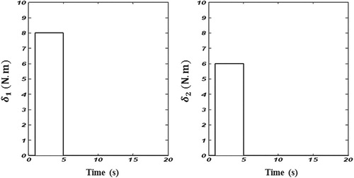
Simulation results are given by considering ${\overline{m}}_1=2.33$, ${\overline{m}}_2=5.33$, ${\overline{m}}_3=2$, ${\overline{m}}_4=3$, ${\overline{m}}_5=2$ and $K_u=Diag\left\{5,10\right\}$. Furtheremore, $x_0=\left[1.57,0,0,0\right]$ and $q_d=\left[1,0.5\right]$ are initial conditions and the desired value of the angular positions of the system, respectively. The applied external disturbance vector $\delta \text{(}t\text{)}=[{\delta }_{\text{1}}\text{(}t\text{)},{\delta }_{\text{2}}\text{(}t\text{)}{]}^T$ are illustrated in Figure 2.

Figure 2. Time response of applied disturbance inputs.

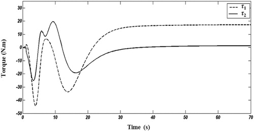
The time-responses of angular positions are shown in Figure 3. As seen, the proposed controller has a robust manner in the face of external disturbances and the angular positions move toward their desired values. The time responses of the applied control vector are also illustrated in Figure 4 where $u\left(t\right)=[u_1\left(t\right),u_2\left(t\right){]}^T=[{\tau }_1\left(t\right),{\tau }_2\left(t\right){]}^T$

Figure 3. Time responses of angular positions of the 2-link robot manipulator system.

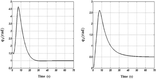
Figure 4. Time responses of control inputs.

7. Construction of PCH form in the presence of parametric uncertainties

In this section, it is intended to design a control law such that in addition to disturbance attenuation be robust against parametric uncertainties of the system. For this purpose, it is necessary to transform equations of the system with parametric uncertainty to PCH structure. Dynamic equations of a system with uncertainty is similar to (3). In this case, it is assumed that matrix $B\left(q\right)$ contains unknown parameters.

Assumption 7.1:

The unknown part of $B\left(q\right)$ is linearly dependent to the unknown vector $\theta \in {\mathbb{R}}^l$. In the other word, the matrix $\varphi \left(q\right)\in {\mathbb{R}}^{n\times l}$ exists such that: (39) $B\left(q\right)=B_0\left(q\right)+\varphi \left(q\right)\theta$(39) where $B_0\left(q\right)$ is the known separable part.

In this case, the Hamiltonian function of the system is considered as follows: (40) $H\left(q,p,\hat{\theta }\right)=K\left(q,p\right)+V_v\left(q\right)+\frac{\text{1}}{\text{2}}(\hat{\theta }\left(t\right)-\theta {)}^T\mathrm{\Psi }\left(\hat{\theta }\left(t\right)-\theta \right)$(40) in which $\hat{\theta }\left(t\right)$ is the estimated value of $\theta$ which will be obtained through the appropriate adaptation law. Moreover, $K\left(q,p\right)$ and $V_v\left(q\right)$ represent the kinetic energy (defined in (6)) and the virtual potential energy of the system where $V_v\left(q\right)$ is defined as (41) $V_v\left(q\right)=\frac{\text{1}}{\text{2}}(q-q_d{)}^T\mathrm{\Lambda }\left(q-q_d\right)$(41)

Furthermore, $\mathrm{\Psi }$ $\in {\mathbb{R}}^{l\times l}$ and $\mathrm{\Lambda }\in {\mathbb{R}}^{n\times n}$ are positive-definite matrixes. The following pre-feedback law transforms system equations to the desired PCH structure: (42) $\begin{array}{rl}u\left(t\right)& =G^{-1}\left(q\right)\left[B_0\left(q\right)-\mathrm{\Lambda }\left(q-q_d\right)\right.\\ & +\left.\varphi \left(q\right)\hat{\theta }-K_u\dot{q}\left(t\right)\right]+u^{\mathrm{\prime }}\end{array}$(42) with the following adaptation law: (43) $\begin{array}{rl}\hat{\dot{\theta }}\left(t\right)& =-{\mathrm{\Psi }}^{-\text{1}}{\varphi }^T\left(q\right)\dot{q}\\ & =-{\mathrm{\Psi }}^{-\text{1}}{\varphi }^T\left(q\right)\frac{\mathrm{\partial }H\left(q,p,\hat{\theta }\right)}{\mathrm{\partial }p}\end{array}$(43) where $K_u\in {\mathbb{R}}^{n\times n}$ is a positive-definit matrix and must be determined. Moreover, $u^{\mathrm{\prime }}$ is an additive control term and is designed in the following such that guarantees the satisfaction of the $H_{\mathrm{\infty }}$ performance index.

According to (40) and (41) and by applying Lemma 4.1: (44) $\begin{array}{rl}\frac{H\left(q,p,\hat{\theta }\right)}{\mathrm{\partial }q}& =\frac{\text{1}}{\text{2}}\left(I_n\otimes p^T\right)\left({\mathrm{\Gamma }}_n\frac{\mathrm{\partial }{M}^{-1}}{\mathrm{\partial }q}\right)p+\frac{\mathrm{\partial }{V}_v\left(q\right)}{\mathrm{\partial }q}\\ & =\frac{1}{2}\left(I_n\otimes p^T\right)\left({\mathrm{\Gamma }}_n\frac{\mathrm{\partial }{M}^{-1}}{\mathrm{\partial }q}\right)p+\mathrm{\Lambda }\left(q-q_d\right)\end{array}$(44) Furthermore, $\frac{\mathrm{\partial }H\left(q,p,\hat{\theta }\right)}{\mathrm{\partial }p}=M^{-1}p=\dot{q}$, thus $p=M\dot{q}$. Therefore, according to system Equations (3) and the relation (38), it is concluded that: (45) $\begin{array}{rl}\dot{p}& =\dot{M}\left(q\right)\dot{q}+M\left(q\right)\ddot{q}\\ & =\dot{M}\left(q\right)\dot{q}-C\left(q,\dot{q}\right)\dot{q}-B\left(q\right)+G\left(q\right)u\left(t\right)\\ & =\dot{M}\left(q\right)\dot{q}-C\left(q,\dot{q}\right)\dot{q}-B_0\left(q\right)-\varphi \left(q\right)\theta +G\left(q\right)u\left(t\right)\end{array}$(45) By substituting the control law (42) into (45), the following relation is obtained: (46) $\begin{array}{rl}\dot{p}& =\left(\dot{M}\left(q\right)-C\left(q,\dot{q}\right)-K_u\right)\dot{q}\\ & +\varphi \left(q\right)\left(\hat{\theta }\left(t\right)-\theta \right)-\mathrm{\Lambda }\left(q-q_d\right)+G\left(q\right)u^{\mathrm{\prime }}\left(t\right)\end{array}$(46) Since $\frac{\mathrm{\partial }H\left(q,p,\hat{\theta }\right)}{\mathrm{\partial }\hat{\theta }}=\left(\hat{\theta }\left(t\right)-\theta \right),$ the above relation can be rewritten as follows: (47) $\begin{array}{rl}\dot{p}& =\left(\dot{M}\left(q\right)-C\left(q,\dot{q}\right)-K_u\right)\dot{q}\\ & +\varphi \left(q\right){\mathrm{\Psi }}^{-1}\frac{\mathrm{\partial }H\left(q,p,\hat{\theta }\right)}{\mathrm{\partial }\hat{\theta }}-\mathrm{\Lambda }\left(q-q_d\right)+G\left(q\right)u^{\mathrm{\prime }}\left(t\right)\end{array}$(47) Considering the relation (47) beside the relation $\dot{q}=\frac{\mathrm{\partial }H\left(q,p,\hat{\theta }\right)}{\mathrm{\partial }p}$ and the adaptation law (47), one may write (48) $\begin{array}{rl}\left[\begin{array}{c}\dot{q}\\ \dot{p}\\ \hat{\dot{\theta }}\end{array}\right]& =\left[\begin{array}{ccc}\text{0}& I_n& \text{0}\\ -I_n& K_C\left(q,p\right)-K_u& \varphi \left(q\right){\mathrm{\Psi }}^{-1}\\ \text{0}& -{\mathrm{\Psi }}^{-1}{\varphi }^T\left(q\right)& \text{0}\end{array}\right]\left[\begin{array}{c}\frac{\mathrm{\partial }H\left(q,p,\hat{\theta }\right)}{\mathrm{\partial }q}\\ \frac{\mathrm{\partial }H\left(q,p,\hat{\theta }\right)}{\mathrm{\partial }p}\\ \frac{\mathrm{\partial }H\left(q,p,\hat{\theta }\right)}{\mathrm{\partial }\hat{\theta }}\end{array}\right]\\ & +\left[\begin{array}{c}\text{0}\\ G\left(q\right)\\ \text{0}\end{array}\right]u^{\mathrm{\prime }}\end{array}$(48) in which: (49) $\begin{array}{rl}{K}_C\left(q,p\right)& =\dot{M}\left(q\right)-C\left(q,\dot{q}\right)\\ & +\frac{\text{1}}{\text{2}}\left(I_n\otimes p^T\right)\left({\mathrm{\Gamma }}_n\frac{\mathrm{\partial }{M}^{-1}}{\mathrm{\partial }q}\right)M\left(q\right)\end{array}$(49) and similar to the previous discussion $K_C\left(q,p\right)\equiv 0$. By defining: (50) $x=\left[\begin{array}{c}q\\ p\\ \hat{\theta }\end{array}\right]$(50) equations of system (48) by considering the parametric uncertainties in the model are obtained as (51) $\dot{x}=\left[J\left(x\right)-R\left(x\right)\right]\frac{\mathrm{\partial }H\left(x\right)}{\mathrm{\partial }x}+g_c{u}^{\mathrm{\prime }}$(51) where (52) $\begin{array}{rl}J\left(x\right)& =\left[\begin{array}{ccc}0& I_n& 0\\ -I_n& 0& \varphi \left(q\right){\mathrm{\Psi }}^{-1}\\ 0& -{\mathrm{\Psi }}^{-1}{\varphi }^T\left(q\right)& 0\end{array}\right]\\ R\left(x\right)& =\left[\begin{array}{ccc}0& 0& 0\\ 0& K_u& 0\\ 0& 0& 0\end{array}\right]\\ g_c& =\left[\begin{array}{c}0\\ G\left(q\right)\\ 0\end{array}\right]\end{array}$(52) It is obvious that $J\left(x\right)=-J^T\left(x\right)$ and $R\left(x\right)=R^T\left(x\right)\ge 0$.

8. Design of the energy-based adaptive ${\mathit{H}}_{\mathrm{\infty }}$ controller

In this section, by means of the achieved PCH structure in the previous section, a control law is designed for the system to attenuate the ${\mathcal{L}}_2$ disturbances. The obtained PCH structure (51) by considering disturbance in the system changes to: (53) $\left\{\begin{array}{l}\dot{x}=\left[J\left(x\right)-R\left(x\right)\right]\frac{\mathrm{\partial }H\left(x\right)}{\mathrm{\partial }x}+g_c{u}^{\mathrm{\prime }}+g_d\delta \\ y=h\left(x\right)g_c^T\left(x\right)\frac{\mathrm{\partial }H\left(x\right)}{\mathrm{\partial }x}\end{array}\right.$(53) in which $g_d=[0I_{n}0{]}^T$.

The task is the design of control law $u^{\mathrm{\prime }}\left(t\right)$ for the system (53) such that $H_{\mathrm{\infty }}$ disturbance attenuation property is satisfied for the closed-loop system. In this regard, the following theorem is given and proved.

Theorem 8.1:

For a defined disturbance attenuation ratio $\gamma >0$, if the following inequality holds: (54) $R\left(x\right)-\frac{1}{2{\gamma }^2}{g}_d{g}_d^T\ge 0$(54) Then, control law (55) leads to ${\mathcal{L}}_2$ disturbance attenuation for the system (53): (55) $u^{\mathrm{\prime }}=-\frac{1}{2}\left(g_c^{†}Q+h{\left(x\right)}^{T}h\left(x\right)g_c^T\right)\frac{\mathrm{\partial }H\left(x\right)}{\mathrm{\partial }x}$(55) where $Q$ is a positive-definite matrix.

Proof:

Applying the control law (55) to the system (53) gives the following closed-loop equations: (56) $\left\{\begin{array}{l}\dot{x}=\left[J\left(x\right)-R\left(x\right)\right]\frac{\mathrm{\partial }H\left(x\right)}{\mathrm{\partial }x}\\ -\frac{1}{2}\left(Q+g_{c}h{\left(x\right)}^{T}h\left(x\right)g_c^T\right)\frac{\mathrm{\partial }H\left(x\right)}{\mathrm{\partial }x}+g_d\delta \\ y=h\left(x\right)g_c^T\left(x\right)\frac{\mathrm{\partial }H\left(x\right)}{\mathrm{\partial }x}\end{array}\right.$(56) Choosing the Hamiltonian function of the system as the Lyapunov function candidate and taking its derivative along trajectories of system (56) yields to: (57) $\begin{array}{rl}\dot{H}\left(x\right)& =\frac{{\mathrm{\partial }}^{T}H\left(x\right)}{\mathrm{\partial }x}\dot{x}\\ & =\frac{{\mathrm{\partial }}^{T}H\left(x\right)}{\mathrm{\partial }x}\left[J\left(x\right)-R\left(x\right)\right]\frac{\mathrm{\partial }H\left(x\right)}{\mathrm{\partial }x}\\ & +\frac{{\mathrm{\partial }}^{T}H\left(x\right)}{\mathrm{\partial }x}\left(-\frac{1}{2}\left(Q+g_{c}h{\left(x\right)}^{T}h\left(x\right)g_c^T\right)\right.\frac{\mathrm{\partial }H\left(x\right)}{\mathrm{\partial }x}\\ & +\frac{{\mathrm{\partial }}^{T}H\left(x\right)}{\mathrm{\partial }x}{g}_d\delta \end{array}$(57) Since $J\left(x\right)$ is a skew symmetric matrix, then $\frac{{\mathrm{\partial }}^{T}H\left(x\right)}{\mathrm{\partial }x}J\left(x\right)\frac{\mathrm{\partial }H\left(x\right)}{\mathrm{\partial }x}=0$. therefore: (58) $\begin{array}{rl}\dot{H}\left(x\right)& =\frac{{\mathrm{\partial }}^{T}H\left(x\right)}{\mathrm{\partial }x}\left(-R\left(x\right)-\frac{1}{2}\left(Q+g_{c}h{\left(x\right)}^{T}h\left(x\right)g_c^T\right)\right)\\ & \times \frac{\mathrm{\partial }H\left(x\right)}{\mathrm{\partial }x}+\frac{{\mathrm{\partial }}^{T}H\left(x\right)}{\mathrm{\partial }x}{g}_d\delta \end{array}$(58) For $Q>0$ then $\left(-\frac{1}{2}\frac{{\mathrm{\partial }}^{T}H\left(x\right)}{\mathrm{\partial }x}Q\frac{\mathrm{\partial }H\left(x\right)}{\mathrm{\partial }x}\right)\le 0$. Therefore (58) results in: (59) $\begin{array}{rl}\dot{H}\left(x\right)\le & -\frac{{\mathrm{\partial }}^{T}H\left(x\right)}{\mathrm{\partial }x}R\left(x\right)\frac{\mathrm{\partial }H\left(x\right)}{\mathrm{\partial }x}-\frac{1}{2}\frac{{\mathrm{\partial }}^{T}H\left(x\right)}{\mathrm{\partial }x}{g}_{c}h(x{)}^{T}h\left(x\right)g_c^T\\ & \times \frac{\mathrm{\partial }H\left(x\right)}{\mathrm{\partial }x}+\frac{{\mathrm{\partial }}^{T}H\left(x\right)}{\mathrm{\partial }x}{g}_d\delta \end{array}$(59) according to the output defined for the system (56): (60) $\dot{H}\left(x\right)\le -\frac{{\mathrm{\partial }}^{T}H\left(x\right)}{\mathrm{\partial }x}R\left(x\right)\frac{\mathrm{\partial }H\left(x\right)}{\mathrm{\partial }x}-\frac{1}{2}{y}^T\text{y}+\frac{{\mathrm{\partial }}^{T}H\left(x\right)}{\mathrm{\partial }x}{g}_d\delta$(60) since $y^T\text{y}=\parallel y{\parallel }^2$ and by adding and subtracting expressions $\frac{1}{2{\gamma }^2}\frac{{\mathrm{\partial }}^{T}H\left(x\right)}{\mathrm{\partial }x}{g}_d{g}_d^T\frac{\mathrm{\partial }H\left(x\right)}{\mathrm{\partial }x}$ and $\frac{{\gamma }^2}{2}\parallel \delta {\parallel }^2$: (61) $\begin{array}{rl}\dot{H}\left(x\right)\le & -\frac{{\mathrm{\partial }}^{T}H\left(x\right)}{\mathrm{\partial }x}R\left(x\right)\frac{\mathrm{\partial }H\left(x\right)}{\mathrm{\partial }x}-\frac{1}{2}||y|{|}^2+\frac{{\mathrm{\partial }}^{T}H\left(x\right)}{\mathrm{\partial }x}{g}_d\delta \\ & +\left(\frac{1}{2{\gamma }^2}\frac{{\mathrm{\partial }}^{T}H\left(x\right)}{\mathrm{\partial }x}{g}_d{g}_d^T\frac{\mathrm{\partial }H\left(x\right)}{\mathrm{\partial }x}\right.\\ & -\frac{1}{2{\gamma }^2}\frac{{\mathrm{\partial }}^{T}H\left(x\right)}{\mathrm{\partial }x}{g}_d{g}_d^T\left.\frac{\mathrm{\partial }H\left(x\right)}{\mathrm{\partial }x}\right)\\ & +\left(\frac{{\gamma }^2}{2}{||\delta ||}^2-\frac{{\gamma }^2}{2}{||\delta ||}^2\right)\end{array}$(61) grouping the right-hand side expressions of (61) yield to: (62) $\begin{array}{rl}\dot{H}\left(x\right)\le & -\frac{{\mathrm{\partial }}^{T}H\left(x\right)}{\mathrm{\partial }x}R\left(x\right)\frac{\mathrm{\partial }H\left(x\right)}{\mathrm{\partial }x}+\frac{1}{2{\gamma }^2}\frac{{\mathrm{\partial }}^{T}H\left(x\right)}{\mathrm{\partial }x}{g}_d{g}_d^T\frac{\mathrm{\partial }H\left(x\right)}{\mathrm{\partial }x}\\ & +\left(-\frac{1}{2{\gamma }^2}\frac{{\mathrm{\partial }}^{T}H\left(x\right)}{\mathrm{\partial }x}{g}_d{g}_d^T\frac{\mathrm{\partial }H\left(x\right)}{\mathrm{\partial }x}\right.\\ & -\frac{{\gamma }^2}{2}{||\delta ||}^2\left.+\frac{{\mathrm{\partial }}^{T}H\left(x\right)}{\mathrm{\partial }x}{g}_d\delta \right)\\ & +\left(\frac{{\gamma }^2}{2}{||\delta ||}^2-\frac{1}{2}{||y||}^2\right)\end{array}$(62) Since, $\begin{array}{rl}\left||\gamma \delta -\frac{1}{\gamma }{g}_d^T\frac{\mathrm{\partial }H\left(x\right)}{\mathrm{\partial }x}\right|{|}^2& =\frac{1}{{\gamma }^2}\frac{{\mathrm{\partial }}^{T}H\left(x\right)}{\mathrm{\partial }x}{g}_d{g}_d^T\frac{\mathrm{\partial }H\left(x\right)}{\mathrm{\partial }x}\\ & +{\gamma }^2||\delta |{|}^2-2\frac{{\mathrm{\partial }}^{T}H\left(x\right)}{\mathrm{\partial }x}{g}_d\delta ,\end{array}$The inequality (62) can be represented as (63) $\begin{array}{rl}\dot{H}\left(x\right)\le & -\frac{{\mathrm{\partial }}^{T}H\left(x\right)}{\mathrm{\partial }x}\left[R\left(x\right)-\frac{1}{2{\gamma }^2}{g}_d{g}_d^T\right]\frac{\mathrm{\partial }H\left(x\right)}{\mathrm{\partial }x}\\ & -\frac{1}{2}\left||\gamma \delta -\frac{1}{\gamma }{g}_d^T\frac{\mathrm{\partial }H\left(x\right)}{\mathrm{\partial }x}\right|{|}^2+\frac{1}{2}\left({\gamma }^2{||\delta ||}^2-{||y||}^2\right)\end{array}$(63) According to relation (54), $\left(\frac{{\mathrm{\partial }}^{T}H\left(x\right)}{\mathrm{\partial }x}\left[R\left(x\right)-\frac{1}{2{\gamma }^2}{g}_d{g}_d^T\right]\right.\left.\frac{\mathrm{\partial }H\left(x\right)}{\mathrm{\partial }x}\right)\ge 0$. Since the first and the second expressions of the right-hand side of (63) are non-positive, thus, the following inequality is obtained: (64) $\dot{H}\left(x\right)\le \frac{1}{2}\left({\gamma }^2{||\delta ||}^2-{||y||}^2\right)$(64) Taking an integral on both sides of (64) gives: (65) $H\left(x\left(\mathrm{\infty }\right)\right)-H\left(x\left(0\right)\right)\le \frac{1}{2}\left({\gamma }^2\underset{0}{\overset{\mathrm{\infty }}{\int }}{||\delta \left(t\right)||}^{2}dt-\underset{0}{\overset{\mathrm{\infty }}{\int }}{||y\left(t\right)||}^{2}dt\right)$(65) since $H\left(x\right)$ is positive-definite and by assuming that $H\left(x\left(0\right)\right)=0$, the relation (65) leads to: (66) $0\le \frac{1}{2}\left({\gamma }^2\underset{0}{\overset{\mathrm{\infty }}{\int }}{||\delta ||}^{2}dt-\underset{0}{\overset{\mathrm{\infty }}{\int }}{||y||}^{2}dt\right)$(66) Therefore, it is inferred that: (67) ${\int }_0^{\mathrm{\infty }}||y\left(t\right)|{|}^{2}dt\le {\gamma }^2{\int }_0^{\mathrm{\infty }}||\delta \left(t\right)|{|}^{2}dt$(67) which means that the $H_{\mathrm{\infty }}$ performance index is satisfied for the closed-loop system. This completes the proof.

In what follows, the effectiveness of the proposed adaptive controller in attenuation of external disturbances is shown through simulations.

9. Design of nonlinear adaptive ${\mathit{H}}_{\mathrm{\infty }}$ controller for 2-link robot manipulator

In order to investigate the performance of the proposed adaptive controller, simulations are taken on the previous 2-link robot manipulator. In this case, $m_p$ is considered as an unknown parameter and one has (68) $\begin{array}{rl}{B}_0\left(q\right)& =\left[\begin{array}{c}(m_1{l}_{c2}+m_2{l}_1)gcos{q}_1+m_2{l}_{c2}g\text{cos}\left(q_1+q_2\right)\\ m_2{l}_{c2}g\text{cos}\left(q_1+q_2\right)\end{array}\right]\\ \varphi \left(q\right)& =\left[\begin{array}{c}{l}_{1}gcos{q}_1+l_{2}g\text{cos}\left(q_1+q_2\right)\\ l_{2}g\text{cos}\left(q_1+q_2\right)\end{array}\right]\end{array}$(68) and $\begin{array}{rl}B\left(q\right)& =B_0\left(q\right)+\theta \varphi \left(q\right)\\ & =B_0\left(q\right)+m_p\varphi \left(q\right)\end{array}$where $\theta =m_p$. Simulations are done by similar parameters and disturbance inputs (refer to Figure 2) as those considered in Section 6. The demanded performance of the proposed adaptive controller in moving the system to the desired angular position despite disturbance inputs and parametric uncertainty. Figure 5 shows the time-responses of the angular positions. As seen the proposed energy-based control has a robust manner and the control goal is achieved in the presence of parametric uncertainty and external disturbances. The time-responses of control inputs are also illustrated in Figure 6.

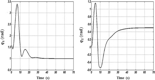
Figure 5. Time responses of angular positions of the 2-link robot manipulator system with parametric uncertainty.

Figure 6. Time responses of control inputs $[u_1\left(t\right),u_2\left(t\right){]}^T=[{\tau }_1\left(t\right),{\tau }_2\left(t\right){]}^T$ of the 2-link robot manipulator system with parametric uncertainty.

10. Conclusion

This paper studied the energy-based $H_{\mathrm{\infty }}$ controller for $n$-degree of freedom mechanical systems. Two different cases were considered and two theorems were given to guarantee the disturbance attenuation and satisfication of the $H_{\mathrm{\infty }}$ performance index based on the Hamiltonian function. In the case of parametric uncertainties, the adaptive approach was also used to obtain a robust manner. Moreover, simulation results on a 2-link robot manipulator were provided to evaluate the performance of proposed controllers in attenuation of applied ${\mathcal{L}}_2$ disturbances. Studying the proposed method based on output feedback or observer-based control are suggested for future works.

Disclosure statement

No potential conflict of interest was reported by the authors.

References

- Acho, L., Orlov, Y., & Solis, V. (2001). Non-linear measurement feedback H∞-control of time-periodic systems with application to tracking control of robot manipulators. International Journal of Control, 74(2), 190–198. doi: 10.1080/00207170150203516
- Asadinia, M. S., & Binazadeh, T. (2019). Finite-time stabilization of descriptor time-delay systems with one-sided Lipschitz nonlinearities: Application to partial element equivalent circuit. Circuits, Systems, and Signal Processing. doi: 10.1007/s00034-019-01129-7
- Binazadeh, T., & Shafiei, M. H. (2016). Novel approach in nonlinear autopilot design. Journal of Aerospace Engineering, 29(1), 04015017. doi: 10.1061/(ASCE)AS.1943-5525.0000500
- Chavez Guzmán, C. A., Aguilar Bustos, L. T., & Mérida Rubio, J. O. (2015). Analysis and synthesis of global nonlinear controller for robot manipulators. Mathematical Problems in Engineering, 2015, 410873. doi: 10.1155/2015/410873
- Chung, W., Fu, L. C., & Hsu, S. H. (2008). Motion control. London: Springer.
- Delgado, S., & Kotyczka, P. (2016). Energy shaping for position and speed control of a wheeled inverted pendulum in reduced space. Automatica, 74, 222–229. doi: 10.1016/j.automatica.2016.07.045
- Erol, B., & Delibaşı, A. (2018). Fixed-order H∞ controller design for MIMO systems via polynomial approach. Transactions of the Institute of Measurement and Control, 41(7), 1985–1992. doi: 10.1177/0142331218792411
- Ge, S. S., & Harris, C. J. (1998). Adaptive neural network control of robotic manipulators. Singapore: World Scientific.
- Gholami, H., & Binazadeh, T. (2019a). Observer-based H∞ finite-time controller for time-delay nonlinear one-sided Lipschitz systems with exogenous disturbances. Journal of Vibration and Control, 25(4), 806–819. doi: 10.1177/1077546318802422
- Gholami, H., & Binazadeh, T. (2019b). Robust finite-time H∞ controller design for uncertain one-sided lipschitz systems with time-delay and input amplitude constraints. Circuits, Systems, and Signal Processing, 38(7), 3020–3040. doi: 10.1007/s00034-018-01018-5
- Hakimi, A. R., & Binazadeh, T. (2017). Robust generation of limit cycles in nonlinear systems: Application on two mechanical systems. Journal of Computational and Nonlinear Dynamics, 12(4), 041013. doi: 10.1115/1.4035190
- Kelly, R., Santibanez, V., & Loria, A. (2005). Control of robot manipulators in joint space. London: Springer.
- Khalil, H. K. (2014). Nonlinear control. Upper Saddle River, NJ: Prentice Hall.
- Krstic, M., & Deng, H. (1998). Stabilization of nonlinear uncertain systems. London: Springer.
- Li, L., & Liao, F. (2018). Design of a robust H∞ preview controller for a class of uncertain discrete-time systems. Transactions of the Institute of Measurement and Control, 40(8), 2639–2650. doi: 10.1177/0142331217708239
- Maschke, B., & Schaft, A. V. (1992). Port-controlled Hamiltonian systems: Modeling origins and system theoretic properties. IFAC Symposium on NOLCOS, 25(13), 359–365.
- Orlov, Y. V., & Aguilar, L. T. (2004). Non-smooth H∞-position control of mechanical manipulators with frictional joints. International Journal of Control, 77(11), 1062–1069. doi: 10.1080/0020717042000273087
- Orlov, Y. V., & Aguilar, L. T. (2014). Advanced H∞ control: Towards nonsmooth theory and applications. New York, NY: Birkhäuser.
- Ortega, R., Loria, A., Nicklasson, J., & Sira-Ramirez, H. (1998). Passivity-based control of Euler-lagrange systems. London: Springer.
- Ortega, R., van der Schaft, A., Maschke, B., & Escobar, G. (2002). Interconnection and damping assignment passivity-based control of port controlled Hamiltonian systems. Automatica, 38(4), 585–596. doi: 10.1016/S0005-1098(01)00278-3
- Sato, K., Yanagi, M., & Tsuruta, K. (2011). Adaptive H∞ trajectory control of nonholonomic mobile robot with compensation of input uncertainty. IEEE international Conference on Control Applications (CCA), Denver, CO (pp. 699–705).
- Shafiei, M. H., & Binazadeh, T. (2014). Movement control of a variable mass underwater vehicle based on multiple-modeling approach. Systems Science & Control Engineering: An Open Access Journal, 2(1), 335–341. doi: 10.1080/21642583.2014.901929
- Shafiei, M. H., & Binazadeh, T. (2015). Application of neural network and genetic algorithm in identification of a model of a variable mass underwater vehicle. Ocean Engineering, 96, 173–180. doi: 10.1016/j.oceaneng.2014.12.021
- Subbotin, A. I. (1995). Generalized solutions of first-order PDE’s—The dynamical optimization perspective. Boston, MA: Birkhäuser.
- Valentinis, F., Donaire, A., & Perez, T. (2015). Energy-based motion control of a slender hull unmanned underwater vehicle. Ocean Engineering, 104, 604–616. doi: 10.1016/j.oceaneng.2015.05.014
- van der Schaft, A. J. (2001). L2-gain analysis of nonlinear systems and nonlinear state feedback H∞ control. IEEE Transactions on Automatic Control, 37(6), 770–784. doi: 10.1109/9.256331
- Wang, Y., & Ge, S. S. (2008). Augmented Hamiltonian formulation and energy-based control design of uncertain mechanical systems. IEEE Transactions on Control Systems Technology, 16(2), 202–213. doi: 10.1109/TCST.2007.903367
- Wang, Y., Yang, X., & Yan, H. (2019). Reliable fuzzy tracking control of near-space hypersonic vehicle using aperiodic measurement information. IEEE Transactions on Industrial Electronics. doi: 10.1109/TIE.2019.2892696
- Wu, Y., & Lu, R. (2018). Event-based control for network systems via integral quadratic constraints. IEEE Transactions on Circuits and Systems I: Regular Papers, 65(4), 1386–1394. doi: 10.1109/TCSI.2017.2748971
- Wu, Y., Lu, R., Shi, P., Su, H., & Wu, Z. G. (2018). Analysis and design of synchronization for heterogeneous network. IEEE Transactions on Cybernetics, 48(4), 1253–1262. doi: 10.1109/TCYB.2017.2688407
- Yang, S., & Xian, B. (2019). Energy-based nonlinear adaptive control design for the quadrotor UAV system with a suspended payload. IEEE Transactions on Industrial Electronics. doi: 10.1109/TIE.2019.2902834
- Zheng, Z., Zhu, M., Zuo, Z., & Yan, K. (2015). Controlled Lagrangians control for a quadrotor helicopter. 27th Chinese Control and Decision Conference (CCDC), Qingdao, China (pp. 6097–6102).