Ship target detection of unmanned surface vehicle base on EfficientDet

Abstract

The autonomous navigation of unmanned surface vehicles (USV) depends mainly on effective ship target detection to the nearby water area. The difficulty of target detection for USV derives from the complexity of the external environment, such as the light reflection and the cloud or mist shield. Accordingly, this paper proposes a target detection technology for USV on the basis of the EfficientDet algorithm. The ship features fusion is performed by Bi-directional Feature Pyra-mid Network (BiFPN), in which the pre-trained EfficientNet via ImageNet is taken as the backbone network, then the detection speed is increased by group normalization. Compared with the Faster-RCNN and Yolo V3, the ship target detection accuracy is greatly improved to 87.5% in complex environments. The algorithm can be applied to the identification of dynamic targets on the sea, which provides a key reference for the autonomous navigation of USV and the military threats assessment on the sea surface.

KEYWORDS:

• Unmanned surface vehicle(USV)
• EfficientDet
• target detection
• group normalization(GN)

1. Introduction

Unmanned surface vehicle (USV) is an autonomous marine equipment used in marine environment monitoring, coastal survey and mapping, military reconnaissance and maritime surveillance, etc. Target detection, as one of the environment sensing technology, plays a key role in the autonomous navigation of USV and is attracted the interest of many scholars.

Deep learning convolutional neural network (CNN) is applied to the perception of unmanned ships to ensure the autonomous navigation of USV. Hinton et al. (2006) proposed firstly the ‘complementary prior’ method to deal with the ‘interpretation-leave’ effect. Ning et al. (2010) adopted an adaptive region merger mechanism with maximum similarity to draw out the target silhouette effectively. Different features were adapted by multiscale convolution filters to improve the feature extraction ability of the mixing layer in Yang et al. (2018). In addition, many scholars carried out intensive studies on ship collision avoidance and autonomous navigation. (2020) used the variable acceptable radius method to calculate the appropriate reference path at the path point. (2017) provided a significant reference by filling the gaps of environmental disturbance in current maritime traffic models. Because of the collision caused by incorrectly interpreting the intents of other vessels, Ma et al. (2021) proposed a deep learning model by adding the accumulated long-term short-term memory (ALSTM), to predict the navigation intention of the intersection waterway. (2020) developed a Bayesian space–time (BS) model to assess collision risk and to help propose management strategies. Yin and Wang (2020) proposed a variable-fuzzy-predictor-based predictive control approach to realize the dynamic trajectory tracking of an autonomous vehicle.

Deep learning was widely applied to ship target detection. A camera scene was fixed on a buoy to detect, locate and track the ship within the line of sight, and the ship detection accuracy reached 88% in Fefilatyev et al. (2012). Wang et al. (2013) presented the method of replacing the dynamic area in the reservoir scene with the adjacent static area to update the background, then created a full ship domain using the region growth algorithm. Li et al. (2016) introduced context information in the sea area to eliminate false positives by the classification according to the bow and hull boundary. Discrete Cosine Transform was used to detect and extract horizontal lines to realize effective visual monitoring of non-fixed surface platforms such as buoys and ships in Zhang et al. (2017). Qi et al. (2019) improved the computational accuracy of Faster R-CNN by image scaling, enhanced the image of ships, and reduced the scope of target search. Huang et al. (2020a) adopted an improved regression deep CNN for ship detection and classification, which improved the recognition rate of small data sets for ship detection and classification.

Nevertheless, the effectiveness of target detection should be improved in the complex environment, such as the light reflection and the screen by cloud or mist. In order to improve the autonomous navigation safety of USV, this paper proposes a target detection technology for USV on the basis of the EfficientDet algorithm (Tan et al., 2019a), which could improve the performance and reduce the model parameters, computation, and training duration greatly compared with the classical networks.

The detailed contributions of this paper are listed as follows. First of all, the EfficientDet algorithm is applied to maritime ship recognition, and it is a new application of marine targets recognition technology. In addition, the ship features fusion is performed by BiFPN that the pre-trained EfficientNet via ImageNet is taken as the backbone network, then the detection speed has increased via group normalization.

The rest of the paper is structured as follows. Section 2 introduces the fundamental theory of the target detection technology mentioned. The data collection and data processing operation is presented in Section 3. Section 4 illuminates the detailed experimental process, evaluation index and model analysis. Finally, the conclusion and future works are given in Section 5.

2. Fundamental theory

2.1. Deep learning

The CNN is formed by adding a convolutional layer and pooling layer upon the traditional full-connection layer neural network (Kunihiko,1980). The process model structure used for deep learning of ship images is shown in Figure 1.

Figure 1. Convolutional neural network structure.

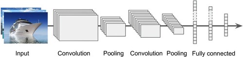
Feature extraction is the most vital function of CNN. As the first layer of the network model, the input layer reads the image data and converts the original image into the corresponding tensor. The size of each image is set to a fixed value. The convolution part, as the second layer of the network, extracts the image features, that is to say, the convolution kernel. The convolution is the weighted sum of two tensors within a certain range. The formula is denoted as (1) $x_i=act(x_i\otimes k_i+b)$(1) where x_i, k_i, and b_i are the feature graph, convolution kernel and bias vector of layer I, respectively, and act(·) is the activation function. ReLU function is often taken as one of the activation functions of the neural network at the convolutional layer. It can be expressed as (2) $f(x)=max(0,x)$(2) where x represents the output vector of the previous layer.

The pooling layer can reduce the parameters and avoid overfitting problems. More specifically, the pooling layer compresses each output feature map into a new feature map. The fully connected layer is a summary of all previous process steps and other related operations to give the final result.

The output of the final layer is essentially a regression model. Predicted probabilities of the output are the final classification result corresponding to the maximum probability.

Convolutional network structure has both automatic feature learning ability and strong classification ability. Therefore, the model can be widely used for ship or naval image recognition by designing a specific network structure (Huang et al., 2020b).

2.2. Feature extraction

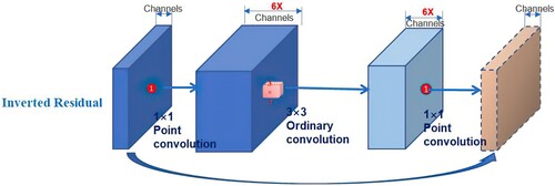
A backbone network with a strong extraction ability is required to recognize small target images of ships with a relative size of less than 0.3. This requires the network to avoid the occurrence of gradient diffusion and to increase the perceptual field of deep feature images as far as possible to improve the detection ability of small targets. A simple requirement was hard to implement technically prior to the emergence of inverted residuals. Inverts residuals (Sandler et al., 2018) were used to solve this problem. The residual module (He et al., 2016) is used for the reuse of data features.

In this paper, input is compressed by 1×1 convolution, then extracted by 3×3 convolution. the number of channels increases through 1×1 convolution, then the input and output also, so as to form a data flow diagram of Compression- Convolution-Expansion. Expansion-Convolution- Compression, in turn, is a data flow graph of inverted residuals, as shown in figure 2.

Figure 2. Data flow graph of inverts residuals module.

2.3. Feature fusion

The multi-scale feature fusion is to aggregate features with different resolutions. The semantic information increases, but the location information decreases gradually with the increasement of sampling times during the network propagation. After 6 times of sub-sampling, the 64×64 pixel target in the original image is only 1×1 in size, so the detection accuracy of the depth feature image for the small-size target gets low.

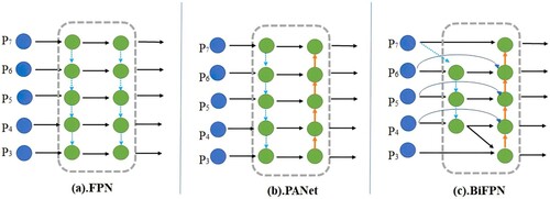
Handling multi-scale features effectively are one of the difficulties in target detection. Pyramid feature layers extracted from the backbone network (Liu et al., 2016) were used as the detectors in earlier studies, even the last layer (Girshick, 2015) was used for classification and location prediction. Multi-scale features are firstly combined using a top-down approach FPN (Lin et al., 2017a). An additional bottom-up path was added to further integrate features based on the Path aggregation Network (PANet, Liu et al., 2018).

EfficientDet optimizes multi-scale feature integration in a more intuitive and interpretable manner, and it uses the BiFPN (Bao & Zhao, 2021), as shown in Figure 3. The following methods are used to improve performance. Firstly, FPN specifically introduced a top-down path via integrating the multi-scale features of levels 3–7 (P3 to P7). Secondly, a bottom-up path is added to the FPN constitutes the PANet. Thirdly, BiFPN with better accuracy and efficiency trade-offs is used.

Figure 3. Feature network design.

2.4. Model scaling

Model Scaling refers to the fact that the model adjusts according to resource constraints. The larger backbone networks and the larger size input images have been applied to identify in the earlier literatures (Ren et al., 2015; He et al., 2017; Redmon & Farhadi, 2018). The scaling of feature networks and box or class prediction networks are also vital for performance considering accuracy and efficiency. The EfficientNet method and the Compound Scaling method are particularly concerned with the EfficientNet model, which scales simultaneously the backbone network, the feature network, and Box/Class predictive network’s resolution ratio, depth, and width (Tan et al., 2019a, 2019b).

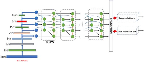
The EfficientDet model is one of the high-performance target detection networks because it has the advantages of simple structure, high efficiency of model extension, and excellent performance. The classification network of EfficientDet is EfficientNet as the backbone network to achieve a good balance of accuracy and speed in the target detection task. EfficientNet is used as the backbone network, BiFPN as the feature network, and the shared class/box prediction net. The EfficientDet model replicates the feature network BiFPN and the class/box net multiple times based on resource constraints. Figure 4 shows the overall architecture of the EfficientDet, which largely follows the single-phase detector paradigm (Liu et al., 2016; Redmon & Farhadi, 2017; Lin et al., 2017b). ImageNet pre-trained EfficientNet as the backbone network is presented. The proposed BiFPN serves as the feature network, which takes level 3–7 features{P3, P4, P5, P6, P7} from the backbone network and repeatedly applies top-down and bottom-up bidirectional feature fusion. These fused features are fed to a class and box network to produce object class and bounding box predictions, respectively. Similar to(Ghiasi et al., 2019), the weights of the class and box network are shared across all levels of features.

Figure 4. EfficientDet architecture.

3. Methodology

The two problems, including insufficient training data and a powerful feature extraction network, need to be solved in Marine ship target identification.

3.1. Data collecting

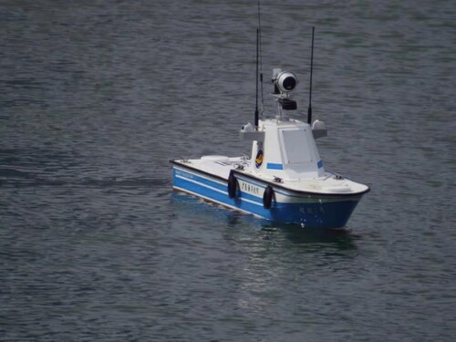
The experiment dataset consists of 122 videos, and the duration of each video is not less than 60 s. The video acquisition task is mainly conducted by a USV of Guangdong Ocean University, named Smart Navigation I as Figure 5.

Figure 5. The USV named Smart navigation I.

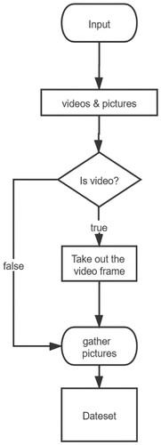
A total of 4000 images were taken out of the captured video by frame operation, and the image data were labeled and annotated, where 90% of which were used for algorithm training plus 10% for testing. The data flow is shown in Figure 6. Most of the photos were taken around 17:00 (GMT+8:00). The water was located at Jinsha Bay or Moon Lake of Haibin Park in Zhanjiang city, China.

Figure 6. Dataset production.

3.2. Normalization

Batch Normalization (BN, Ioffe & Szegedy, 2015) implements a pre-processing operation in the middle of the neural network layers, i.e. the input of the previous layer is normalized before entering the next layer of the network, which can prevent effectively ‘gradient dispersion’ and accelerate the network training. There are two common approaches. One is to take the neurons in a feature map as a feature dimension with parameter r, which could make the number of parameters larger, so this approach is not used in this paper. The other approach of ‘shared parameter’ was adopted here, which means that a whole feature map is considered as a feature dimension, and this feature dimension and the function mapping of neurons share a parameter r. Consequently, we can smoothly calculate and obtain the required mean and variance process in the BN layer during the training.

However, BN has a serious drawback in the experiments including the limited quantities of the training process and video memory, the harder image processing task and the higher hardware requirements. Group Normalization (GN, Wu & He, 2018) that is superior to BN in small-batch training could be employed. The input data of a neural network usually have four dimensions, B (batch), C (channel), H (height) and W (width). GN can be represented by (3) $\{\begin{array}{l}{x}_i={\displaystyle \frac{x_i-{\mu }_i}{{\sigma }_i}}\\ {\mu }_i={\displaystyle \frac{1}{\left({\displaystyle \frac{C}{\text{G}}}\right)HW}}\sum _{c=g{\displaystyle \frac{C}{\text{G}}}}^{(g+1){\displaystyle \frac{C}{\text{G}}}}\sum _{h=1}^H\sum _{w=1}^W{x}_{bchw}\\ \sigma (x)=\sqrt{{\displaystyle \frac{\sum _{c=g{\displaystyle \frac{C}{\text{G}}}}^{(g+1){\displaystyle \frac{C}{\text{G}}}}\sum _{h=1}^H\sum _{w=1}^W{(x_{bchw}-{\mu }_i(x))}^2+\epsilon }{\left({\displaystyle \frac{C}{\text{G}}}\right)H\text{W}}}}\end{array}$(3) where x is used to calculate the tensor of the feature map, i stands for index number, that is $x_i=(x_{iC},x_{iB},x_{iW},x_{iH})$, x_i denotes the tensor after the normalization process. The mean and the standard deviation are denoted by $\mu ,\sigma$, respectively. ϵ is an arbitrarily small constant, $\sigma {}_i\ge 0$. b, c, g, h, and w are the index number, whose range of values are B, C, G, H, W, respectively. The number of artificially set groups is G and $C/G$ counts the number of channels in each group. GN can be implemented by Algorithm 1.

Table

Algorithm 1. Code of GN
def GN (x, gamma, beta, G, eps=1e−5):
# x: input features with shape [B,C,H,W]
# gamma, beta: scale and offset, with shape [1,C,1,1]
# G: number of groups for GN
B, C, H, W = x.shape
x = tf.reshape(x, [B, G, C // G, H, W])
Mean,var = tf.nn.moments(x, [2, 3, 4], keep_dims = True)
x = (x−mean) / tf.sqrt(var + eps)
x = tf.reshape(x, [B, C, H, W])
return x*gamma + beta

3.3. LOSS

The loss functions can be classified into two categories, classification and regression loss. What’s special about the loss functions of the models used here is that there is a margin between positive and negative samples, that is to say, the Anchor with IOU < 0.5 is marked as a negative sample, and the Anchor with IOU > = 0.5 is marked as a positive sample. (IOU, refer to section 4.3). The Smooth Loss role is to calculate the target regression box loss. Focal Loss serves to calculate the cross-entropy loss of the predicted outcome for all unignored categories.

4. Experiments

4.1. Image manipulations

In this paper, the overfitting is overcome by the image enhancement method, which increases the number of data sets and improves the robustness of the model. At the beginning of the experiment, new images are obtained by changing the saturation, brightness, and contrast of the images, cropping or mosaicing the images to gain the new ones, and merging the above-processed images into a part of the dataset. To fully identify the target, the label and annotation of the self-collected dataset are necessary for the process of the experiment. In this study, the target vessel to be identified is marked by rectangles.

4.2. Experimental procedure

According to the designed experimental requirements, the surface ship target detection experiment is carried out within the perspective range of USV, and the experimental steps and technology are given as follows.

Step 1: the experimental USV equipped with a camera does not require external camera equipment, but communication equipment is connected via WIFI. The communication settings are shown in Figure 7.

Figure 7. Communication transmission settings.

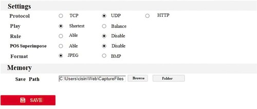
Step 2: the water surface scenes are captured by the camera, and the video data is collected autonomously, simultaneously, which is used for training and testing. The parameters adapted to different scenes are tuned.

Step 3: Video image processing is to take out the identified ship information.Firstly, the image data is taken from the video clip as one frame per second. Secondly, determine the size of the video frame data, then send the data set to the trained algorithm model for identification. Thirdly, synthesize and output the video. The sensory comfort, as well as the basic visual fluency, could be satisfied in the event of 21 frames per second.

4.3. Experimental environment and result

The experimental platform system is Windows 10, and the graphics processing unit (GPU) is NVIDIA GTX2080Ti. The deep learning framework is TensorFlow 2.2.0. The details are shown in Table 1.

Table 1. Running environment of model.

System Environment	Windows 10(64)
CPU	Intel(R)Core(TM) i9-9980XE
GPU	NVIDIA GTX2080Ti
Python	3.7.0
TensorFlow	2.2.0

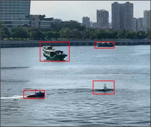
One image of the recognition result is shown in Figure 8.

Figure 8. The image of ship target detection from USV.

4.4. Experimental evaluation and analysis

The evaluation indexes include P (Precision), R (Recall), and AP(Average Precision). These indexes are used to measure the accuracy of target detection. The calculation process is as (4) $\{\begin{array}{l}\text{R = }{\displaystyle \frac{\text{TP}}{\text{FN}+\text{TP}}}\\ \text{AP = }{\int }_0^1\text{P}(\text{R})dR\end{array}$(4) where true positives (TP, IOU≥0.5), false positives (FP, IOU<0.5), false negatives (FN) and true negatives (TN). In practice, the function of P concerning R is discrete, and the Intersection over Union (IOU,$\text{IOU = }\frac{\text{DR}\cap \text{GT}}{\text{DR}\cup \text{GT}}$) between the prediction box and the annotation box is needed. Detection Result (DR) represents the result obtained by the neural network and Ground Result (GR) represents the result of the mark. IOU denotes the degree of overlap and IOU∈[0, 1].

Sufficient training has been done in case of the complex environment. The distinction between complex and simple standards is as follows: the complex environment is mainly concerned with illumination, including strong light and backlight conditions, being shielded by smoke, rain, fog, and image overlap of ships, etc. The other conditions are deemed as the simple background environments ignoring the onshore architectural background. AP50 represents the AP as IOU=0.5.

During the training with the original 8 models, it is found that the feature learning performance of the Le-Net5 model is poor, so this model is abandoned for comparison in the subsequent experiments. The results of seven models are compared to evaluate the EfficientDet application. EfficientDet has developed EfficientDet-D0 to D7, which have the same BiFPN and head but possess a different number of BiFPN and input channels. With the superposition of the network layer side, the speed is reduced, and the precision is improved gradually.

Table 2 gives the comparison of the experimental results. It shows that the EfficientDet-D4 model is only 83.5 MB in size, which is moderate among all the models. The SSD-300 model has many restrictions on the resolution of the input image, although it has achieved the best performance in FPS. When the input image size is constrained within 512×512, the EfficientDet-D0 FPS reached 42.5. The accuracy is lower than the EfficientDet-D3 model. Therefore, the EfficientDet-D4 model adopted in this paper meets the real-time requirement. EfficientDet-D4 is available at 21.4 frames per second, which matches the visual experience requirement.

Table 2. Model comparison.

Model	FPS	Storage size (/MB)	AP50 (Simple)	AP50 (Complex)
EfficientDet-D4	21.4	83.5	0.936	0.875
EfficientDet-D3	34.5	47.9	0.824	0.764
EfficientDet-D0	42.5	16.1	0.792	0.650
Yolo V3	61	235.5	0.72	0.68
SSD-512	37.3	195.0	0.76	0.57
SSD-300	57.0	190.0	0.68	0.54
Faster-RCNN	39.2	119.0	0.66	0.57

5. Conclusion

Ship target detection for USV is difficult under complex environmental conditions such as backlight, strong light, and being shielded by cloud, rain, and fog. The image data set collected by the authors is specially trained under the complex environment in this paper. The calculation time is greatly saved by preprocessing the image prior to training. Marine ship target detection for USV was studied employing the EfficientDet algorithm to overcome the traditional resource consumption problems and improve identification accuracy. The experiment verified that the accuracy rate is 87.5% in the complex background, and 93.6% in a simple one. Future work will focus on improving identification capabilities, classification of ships, and detection of other targets offshore.

Disclosure statement

No potential conflict of interest was reported by the author(s).

Correction Statement

This article has been corrected with minor changes. These changes do not impact the academic content of the article.

Additional information

Funding

This work is supported partially by the National Natural Science Foundation of China [grand number 52171346], the Natural Science Foundation of Guangdong Province [grand number 2021A1515012618], the special projects of key fields (Artificial Intelligence) of Universities in Guangdong Province [grand number 2019KZDZX1035], and program for scientific research start-up funds of Guangdong Ocean University.

References

- Bao, Z. Z., & Zhao, X. J. (2021). Ship detector in SAR images based on EfficientDet without pre-training. Journal of Beijing University of Aeronautics and Astronautics, 47(8), 1644–1672. https://doi.org/10.13700/j.bh.1001-5965.2020.0255
- Fefilatyev, S., Goldgof, D., Shreve, M., & Lembke, C. (2012). Detection and tracking of ships in open sea with rapidly moving buoy-mounted camera system. Ocean Engineering, 54, 1–12. https://doi.org/10.1016/j.oceaneng.2012.06.028.
- Ghiasi, G., Lin, T. Y., Pang, R., & Le, Q. V. (2019). NAS-FPN: Learning Scalable Feature Pyramid Architecture for Object Detection. 2019 IEEE/CVF Conference on Computer Vision and Pattern Recognition, 2019, 7029–7038. https://doi.org/10.1109/CVPR.2019.00720
- Girshick, R. (2015). Fast R-CNN. Proceedings of the IEEE International Conference on Computer Vision, 2015, 1440–1448. https://doi.org/10.1109/ICCV.2015.169
- He, K., Zhang, X., Ren, S., & Sun, J. (2016). Deep residual learning for image recognition. 2016 IEEE Conference on Computer Vision and Pattern Recognition, 2016, 770–778. https://doi.org/10.1109/CVPR.2016.90
- He, K. M., Gkioxari, G., Dollár, P., & Girshick, R. (2017). Mask r-CNN. 2017 IEEE International Conference on Computer Vision, 2017, 2980–2988. https://doi.org/10.1109/ICCV.2017.322
- Hinton, G. E., Osindero, S., & Teh, Y. W. (2006). A fast learning algorithm for deep belief nets. Neural Computation, 18, 1527–1554. https://doi.org/10.1162/neco.2006.18.7.1527.
- Huang, B., He, B., Wu, L., & Lin, Y. (2020a). A deep learning approach to detecting ships from high-resolution aerial remote sensing images. Journal of Coastal Research, 111(SI), 16–20. https://doi.org/10.2112/JCR-SI111-003.1
- Huang, Z., Sui, B., Wen, J., & Jiang, G. (2020b). An intelligent ship image/video detection and classification method with improved regressive deep Convolutional neural network. Complexity, 2020, 1–11. https://doi.org/10.1155/2020/1520872
- Ioffe, S., & Szegedy, C. (2015). Batch normalization: Accelerating deep network training by reducing internal covariate shift. Proceedings of the 32nd International Conference on International Conference on Machine Learning, 37(ICML15), 448–456. https://arxiv.org/abs/1502.03167
- Kunihiko, & Fukushima (1980). Neocognitron: A self-organizing neural network model for a mechanism of Pattern recognition unaffected by shift in position. Biological Cybernetics, 36(4), 193–202. https://doi.org/10.1007/BF00344251
- Li, S., Zhou, Z., Wang, B., & Wu, F. (2016). A novel inshore ship detection via ship head classification and body boundary determination. Proceedings of the IEEE Geoscience and Remote Sensing Letters, 13(12), 1920–1924. https://doi.org/10.1109/LGRS.2016.2618385
- Li, Z., Li, R., & Bu, R. (2020). Path following of underactuated ships based on model predictive control with state observer. Journal of Marine Science and Technology, 26(4). https://doi.org/10.1007/s00773-020-00746-1
- Lin, T. Y., Dollár, P., & Girshick, R. (2017a). Feature pyramid networks for object detection. 2017 IEEE Conference on Computer Vision and Pattern Recognition, 2017, 936–944. https://doi.org/10.1109/CVPR.2017.106
- Lin, T. Y., Goyal, P., Girshick, R., He, K., & Dollár, P.. (2017b). Focal loss for dense object detection. 2017 IEEE International Conference on Computer Vision, 2017, 2999–3007. https://doi.org/10.1109/ICCV.2017.324
- Liu, S., Qi, L., Qin, H., Shi, J., & Jia, J. (2018). Path aggregation network for instance segmentation. 2018 IEEE/CVF Conference on Computer Vision and Pattern Recognition, 2018, 8759–8768. https://doi.org/10.1109/CVPR.2018.00913
- Liu, W., Anguelov, D., Erhan, D., Szegedy, C., Reed, S., & Fu, C. Y.. (2016). SSD: Single shot multi-box detector. Proceedings of the European Conference on Computer Vision,2016. Lecture Notes in Computer Science, 9005, 21–37. https://doi.org/10.1007/978-3-319-46448-0_2
- Ma, J., Jia, C., Shu, Y., Liu, K., & Hu, Y. (2021). Intent prediction of vessels in intersection waterway based on learning vessel motion patterns with early observations. Ocean Engineering, 232(3), 1–14. https://doi.org/10.1016/j.oceaneng.2021.109154
- Ning, J., Zhang, L., Zhang, D., & Wu, C. (2010). Interactive mage segmentation by maximal similarity-based region merging. Pattern Recognition, 43, 445–456. https://doi.org/10.1016/j.patcog.2009.03.004
- Qi, L., Li, B., Chen, L., & Wang, W. (2019). Ship target detection algorithm based on improved Faster R-CNN. Electronics, 8(9), 1–19. https://doi.org/10.3390/electronics8090959
- Redmon, J., & Farhadi, A. (2017). Yolo9000, better, faster, stronger. 2017 IEEE Conference on Computer Vision and Pattern Recognition, 2017, 6517–6525. https://doi.org/10.1109/CVPR.2017.690
- Redmon, J., & Farhadi, A. (2018). Yolov3, An incremental improvement. arXiv preprint arXiv:1804.02767. https://arxiv.org/abs/1804.02767
- Ren, S. Q., He, K. M., Girshick, R., & Sun, J.. (2015). Faster r-CNN: Towards real-time object detection with region proposal networks. IEEE Transactions on Pattern Analysis and Machine Intelligence, 39(6), 1137–1149. https://doi.org/10.1109/TPAMI.2016.2577031
- Sandler, M., Howard, A., Zhu, M., Zhmoginov, A., & Chen, L. C. (2018). Mobilenetv2, inverted residuals, and linear bottlenecks. 2018 IEEE/CVF Conference on Computer Vision and Pattern Recognition, 2018, 4510–4520. https://doi.org/10.1109/CVPR.2018.00474
- Shu, Y., Daamen, W., Ligteringen, H., & Hoogendoorn, S. P. (2017). Influence of external conditions and vessel encounters on vessel behavior in ports and waterways using automatic identification system data. Ocean Engineering, 131(2017), 1–14. https://doi.org/10.1016/j.oceaneng.2016.12.027
- Tan, M., Pang, R., & Le, Q. V. (2019a). EfficientDet: Scalable and efficient object detection. 2020 IEEE/CVF Conference on Computer Vision and Pattern Recognition, 2020, 10778–10787. https://doi.org/10.1109/CVPR42600.2020.01079
- Tan, M. X., Pang, R., & Le, Q. V. (2019b). EfficientDet: Scalable and efficient object detection. 2020 IEEE/CVF Conference on Computer Vision and Pattern Recognition, 2020, 10778–10787. https://doi.org/10.1109/CVPR42600.2020.01079
- Wang, Z. Y., Xie, L., Yan, Z. Z., & Yan, X. P. (2013). Inland ship recognition algorithm based on neighboring static region substitution for background updating. Applied Mechanics and Materials, 416–417, 1233–1238. https://doi.org/10.4028/www.scientific.net/amm.416-417.1233
- Wu, Y. X., & He, K. M. (2018). Group normalization. Proceedings of the European Conference on Computer Vision, 2018(128), 742–755. https://doi.org/10.1007/s11263-019-01198-w
- Yang, Z., Yu, W., Liang, P., Guo, H., Zhang, F., & Ma, J. (2018). Deep transfer learning for military object recognition under small training set conditions. Neural Computing and Applications, 2018(31), 6469–6478. https://doi.org/10.1007/s00521-018-3468-3
- Yin, J. C., & Wang, N. (2020). Predictive trajectory tracking control of autonomous underwater vehicles based on variable fuzzy predictor. International Journal of Fuzzy Systems, 2020(23), 1809–1822. https://doi.org/10.1007/s40815-020-00898-7
- Yu, Y., Chen, L., Shu, Y., & Zhu, W. (2020). Evaluation model and management strategy for reducing pollution caused by ship collision in coastal waters. Ocean & Coastal Management, 203(105446), 1–9. https://doi.org/10.1016/j.ocecoaman.2020.105446
- Zhang, Y., Li, Q. Z., & Zang, F. N. (2017). Ship detection for visual maritime surveillance from non-stationary platforms. Ocean Engineering, 2017(141), 53–63. https://doi.org/10.1016/j.oceaneng.2017.06.022