
ABSTRACT
Very high-resolution satellite stereo images play an important role in cartographical and geomorphological applications, provided that all the processing steps follow strict procedures and the result of each step is carefully assessed. We outline a general process for assessing a reliable analysis of terrain morphometry starting from a GeoEye-1 stereo-pair acquired on an area with different morphological features. The key steps were critically analyzed to evaluate the uncertainty of the results. A number of maps of morphometric features were extracted from the digital elevation models in order to characterize a landslide; on the basis of the contour line and feature maps, we were able to accurately delimit the boundaries of the various landslide bodies.
Introduction
Optical satellites are now able to collect very high-resolution imagery over large land areas with a high level of detail, and the spectral and spatial resolutions of satellite data play a significant role in ensuring the accuracy and reliability of the derived maps.
For instance, the GeoEye, WorldView and Pléiades satellites provide imagery with a ground sampling distance (GSD) of approximately 50 cm in panchromatic mode. Moreover, during 2014, a few satellite companies received permission to collect and sell imagery at up to 25 cm panchromatic and 1.0 m multispectral GSD.
For decades, aerial imagery had been the only approach available for generating digital elevation models (DEMs) over large areas. Although airborne photogrammetric flights with new digital aerial cameras make it possible to capture highly detailed imagery, the drawback is that they require “ad hoc” photogrammetric flights at detailed scale and the handling of a high number of frames.
Unmanned aerial vehicles (UAVs) allow more detailed imagery to be acquired but only over very small areas (Niethammer, James, Rothmund, Travelletti, & Joswig, Citation2012).
Several current satellite missions not only provide high-resolution images but are also able to acquire stereo-images that make it possible to create a DEM (Y. Hu, Cheng, Q. Hu, Cheng, Hu, Li, & Zeng, Citation2011; Jacobsen, Citation2009, Citation2013; Murillo-García et al., Citation2015). Also, various software packages such as ENVI (Exelis), ERDAS (Hexagon Geospatial), Geomatica (PCI Geomatics), SOCET SET (Bae Systems), ArcGIS (ESRI) and many others are extensively used to extract DEMs from very high-resolution stereo-imagery. Therefore, VHR optical satellites are now capable of producing images and hence DEMs that can compete with traditional aerial photogrammetric products (Aguilar, Del Mar Saldaña, & Aguilar, Citation2014; Jacobsen, Citation2011; Yaşa, Erbek, Ulubay, & Özkan, Citation2004).
DEMs, contour line maps, 3D exploration and ortho-rectified images can help us to analyze characteristic terrain features as well as changes in morphometry, provided that these products are reliable and accurate (Agugiaro, Poli, & Remondino, Citation2012; Fraser & Ravanbakhsh, Citation2009; Gómez-Candón, López-Granados, Caballero-Novella, Peña-Barragán, & García-Torres, Citation2012; Guarnieri, Masiero, Vettore, & Pirotti, Citation2015; Meguro & Fraser, Citation2010; Poli & Caravaggi, Citation2016; Poli & Toutin, Citation2012).
Consequently, particular attention must be paid in the creation of a reliable numerical model that correctly describes the topography.
The imagery georeferencing phase is therefore a very important step in ensuring the reliability of the products derived from the imagery (Toutin, Citation2004). For VHR satellite imagery, most researchers recommend the use of either 3D physical or rigorous models (Dolloff & Settergren, Citation2010; Grodecki & Dial, Citation2003) or the vendor supplied rational polynomial coefficients refined through a small number of high accuracy ground control points (GCPs) (Aguilar, Del Mar Saldaña, & Aguilar, Citation2013; Hanley, Yamakawa, & Fraser, Citation2002; Hu, Tao, & Croitoru, Citation2004).
Another frequently used georeferencing method is the rational polynomial function (RPF) model, which requires the availability of a large number of high accuracy GCPs. Numerous GCPs can be quickly acquired from the latest large-scale map, or with a more accurate method like a GNSS survey using the surveying technique positioning service in real time (network real-time kinematic – NRTK), now widespread in many countries. By using the DEM derived from satellite imagery, it is then possible either to directly extract the contour lines or to create a map via image ortho-rectification (Capaldo, Crespi, Fratarcangeli, Nascetti, & Pieralice, Citation2012; Daliakopoulos & Tsanis, Citation2013; Deilami & Hashim, Citation2011; Saldaña, Aguilar, Aguilar, & Fernández, Citation2012).
Geological analyses of terrain morphology are often based on contour lines maps derived from DEMs (Drăguţ & Eisank, Citation2011; Lu, Stumpf, Kerle, & Casagli, Citation2011). Starting from a reliable and accurate DEM, it is possible to extract a number of land-surface parameters, which are useful to accurately delineate and quantify landslides and other similar features using geomorphometrics criteria (Dramis, Citation2009; Hengl & Reuter, 2009). In detail, Geographic Information Systems (GIS) have greatly contributed to the study and mapping of the landforms (Chacón & Corominas, Citation2003; Huabin, Gangjun, Weiya, & Gonghui, Citation2005).
However, apart from Leoni et al. (Citation2009), Li, Zhu and Gold (Citation2005), Wilson and Gallant (Citation2000), few scientific papers or textbooks tackle the elaboration of a DEM suitable for carrying out analysis in packaged software (Shean et al., Citation2016).
A major problem in this sense is the absence of standards for extracting DEMs useful for such analyses. While traditional photogrammetric surveying can count on many codified procedures to produce DEMs and cartography (Hugenholtz et al., Citation2013), similar codings do not seem available for VHR images.
In this work, we have elaborated a VHR stereo pair collected by the GeoEye-1 satellite: the stereoimage covers an area with different morphology where mountainous, partly shadowed zones alternate with hilly and flat ones. A well-known landslide compound, which has been the object of a few geomorphological studies (Calcaterra et al., Citation2014; De Vita, Carratù, La Barbera, & Santoro, Citation2013), affects a small area of the imagery.
The geomorphometrical mapping process has been critically evaluated step by step from the georeferencing phase to the DEM and maps production phases, in order to achieve reliable and accurate products. We produced a number of contour line and features maps in order to better analyze the landslide compound and to delimitate its different bodies. Direct knowledge of both the terrain morphology and the trend of the landslide allows us to directly verify the parameters used to elaborate the DEM.
Study site and material
The GeoEye-1 stereo image pair () reports its characteristics which was captured in reverse scan mode with the panchromatic band and all four multispectral bands recorded. The site covered an area of 110 km2, as shown in .
Table 1. Characteristics of the GeoEye-1 stereo-pair.
Figure 1. One of the two GeoEye-1 images composing the stereo-pair represented in pan-sharpened mode. DATUM is ETRS89, frame ETRF00. The four areas highlighted and marked by letters have been studied in more detail: A mountain area (a), a hilly area (b), a flat area (c) and an area (d) of special geomorphological interest affected by an important active landslide compound system.
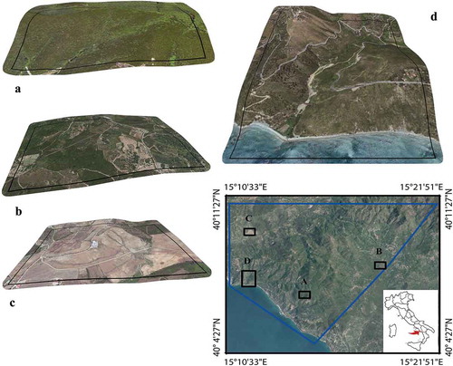
For the analysis described here, only the panchromatic level 1A imagery has been considered. The area covered by the stereo-pair is a coastal area of southern Italy. The topography is highly variable, ranging from sea level to altitudes of over 1000 m. Shrubs and isolated large trees cover most of the area, but there are also a few residential zones and isolated houses.
The whole satellite image was georeferenced and the DEM was extracted. Within the image, we have selected three subareas of different morphologies to study in greater detail. shows a mountain area (A), a hilly area (B) and a flat area (C). Area (D) is of special geomorphological interest as it is affected by an important active landslide compound system (Barbarella, Fiani, & Lugli, Citation2015; De Vita et al., Citation2013).
We carried out a number of tests with both Geomatica ver. 2013.0.0 and Socet Set ver. 5.8.0. They are both software packages that perform a variety of functions related to photogrammetry and remote sensing.
Methods
If the aim of the survey is landscape characterization in order to monitor changes over time, the outcome of any image elaboration step – georeferencing, image matching, DEM extraction and morphometrical feature extraction – should be subjected to critical analysis.
Georeferencing
For geomorphological purposes, the image georeferencing phase is of primary importance. The georeferencing accuracy of high-resolution satellite imagery is not a function of spatial resolution alone, as it is also dependent upon radiometric image quality, satellite platform attitude and the precision of the GCPs survey. The most frequently used georeferencing algorithms are based on rigorous models or on use of RPFs.
In this work, we have tested the physical model embedded within the software Geomatica (called “Toutin’s model”), the physical one embedded in Socet Set (called “rigorous simultaneous”) and the RPF model embedded in Geomatica (called “Rational Function”).
The software user’s guides suggest using only a few points (from 6 to 10 for Geomatica, even less for Socet) to geo-reference the image if the rigorous model is used. This is why we used only a small number of points as GCPs. The remaining were used as check points (CPs) for testing the accuracy of the output (e.g. to evaluate the difference between the value measured on the terrain and that measured on the georeferenced image).
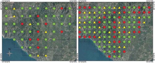
In order to georeference the image, we run a NRTK GPS surveying campaign. To obtain a homogeneous distribution of well-“matched” points, control points were chosen in close proximity to the nodes of a regular grid; grid spacing was fixed while bearing in mind the number of points required for image georeferencing, which depends on the type of mathematical transformation used. The grid was overlaid onto the image and the GCPs position was selected nearby these nodes taking care of choosing “stable” details clearly visible on the image, such as artifacts or natural objects (, left panel). Due to the presence of many mountainous districts, devoid of any stable points that can be easily identified on the image, in some areas, there are no points in correspondence of the grid nodes.
Figure 2. Regular grids have been drawn on the image to obtain a homogeneous distribution of well-“matched” points. Control points have been chosen in close proximity of the nodes of the grid. Green circles indicate areas on the images that are close to visible control points, yellow triangles indicate “bad” points with issue of collimation (since they are located in shady areas of the image), red squares are on the location of grid nodes where it was not possible to find a point to collimate (mountain areas and/or without artifacts). Left panel: GGCPs; right panel: MGCPs. DATUM is ETRS89, frame ETRF00.
In order to design the surveying campaign, it is necessary to consider whether the site offers good road access or it is isolated. In this case, neither a good cellular phone signal nor a good satellite DOP value, which are necessary conditions for the GPS NRTK survey, can be expected.
Thanks to the speed of the GPS measurements, once we had reached the survey area, we decided to measure several neighboring points in order to then choose which could be better collimated on the image and which was the best in terms of measurement quality.
A total of 29 points were deemed suitable for use as either GCPs or CPs in our experimental testing. The position accuracy for the points measured using the NRTK technique is estimated to be better than 10 cm.
Positions were directly obtained in the European Terrestrial Reference System 1989 (ETRS89), the European and National geodetic system, European Terrestrial Reference Frame 2000 (ETRF00).
A few other points were acquired from the latest available map, the Cartografia Tecnica Regionale at a scale of 1:5000. The cost of data acquisition from the map is obviously much lower than with the surveying campaign, so many more points were measured on the map. The point acquisition pattern was designed so as to have a homogeneous distribution (, right panel). We have also taken care to ensure that the points whose coordinates were measured on the map correspond on the image to details that are both stable and well collimable.
Geomatica, if a geocoded map covering the area in the image is available, manages the geometric correction process through an OrthoEngine application which allows us to collect the GCPs directly on the map. The cursor must be positioned exactly over the location in the uncorrected image that we wish to use for control and later over the identical location in the geocoded image map. Good choices are road intersections in built-up areas or sharp river bends in natural environments. We have got our estimate for the elevation from a linear interpolation of the contour lines.
Obviously, the georeferenced map must have the coordinate system you have set for your image in the “set projection” panel.
Regarding the choice of the point location, besides the presence of homologous points on the image and on the map, a further necessary requirement is the possibility to acquire all three of their coordinates on the map with good accuracy; some areas lack points showing these features. The whole process would be improved if it were possible to give 2D (planimetric) and 1D (altimetric) point coordinates separately. Unfortunately, this is not possible as both software packages demand 3D points.
The planimetric root mean square error (RMSE(N,E)) of the map is about 1.2 m and the vertical error RMSE(H) is 0.75 m (Barbarella, Fiani, & Lugli, Citation2017). The accuracy of these points is clearly lower than the one of the points measured directly on the terrain.
In summary, the GCPS used for georeferencing the stereoimage consists of two different sets: GPS GCPs (from now on, called GGCPs) and mapping GCPs (from now on, called MGCPs).
In , the green circles indicate areas on the images near to visible control points, to be measured on the terrain (left panel) or on the map (right panel), the yellow triangles indicate “bad” points with some collimation problems because they are located in shadowed areas of the image and the red squares indicate the location of grid nodes where it has not been possible to find a point to collimate (mountain areas and/or without artifacts).
We should also homogenize the geodetic reference systems used. In our case study, both cartography and NRTK are framed in ETRF00. Therefore, no datum transformation was needed for planimetry whereas the height needs a transformation from ellipsoidal to geoidal using an accurate geoid height model specific to Italy (Pepe & Prezioso, Citation2015).
In order to verify the numerical accuracy of the georeferencing, we provided the residual values computed by the software, i.e. the difference between the adjusted coordinates and the input ones, measured either on the ground or on the map. On the CPs, the software computed the shifts between the measured value of the coordinates and the value measured on the georeferenced image.
DEM extraction
In this phase, we studied the accuracy of the DEMs extracted using stereo-matching techniques from the stereo images. Two commercial software packages – Geomatica and SocetSet – were used for the image processing phases, including DEM extraction.
In both cases, the DEM extraction process makes use of image correlation to find matching features on the two images of a stereo pair, adopting strategies specific to the software used.
Geomatica used a feature-based matching model called normalized cross-correlation matching. This method finds the relative shift between two images by finding the shift that produces the maximum cross-correlation coefficient of the gray values in the images (Geomatics, Citation2010; Lewis, Citation1995).
The software requires epipolar images to extract the DEM, in order to reduce the time necessary to find corresponding points in image matching (Deilami & Hashim, Citation2011). At this stage, it is helpful to add some tie points to improve the digital matching in a few “critical” zones, mainly in the shadowed areas of the mountain slopes. A hierarchical approach using a pyramid of reduced resolution images was the method adopted in order to find these matching features.
In this phase, two parameters need to be chosen: “DEM resolution” (the size of the pixel in the final DEM) and “DEM detail”. Specifically, the latter determines how precisely to represent the terrain in the DEM. Selecting “very high”, “high”, “medium” or “low” determines the time at which to stop the correlation process. In the case of failed correlation, in order to enhance the continuity of the DEM surface, we set the “fill holes” option so as to automatically filter the elevation values by interpolating the failed areas; however, this strongly influences the reliability of the resulting DEM.
With Geomatica, the first tests to verify the DEM accuracy were carried out by varying both the parameter “resolution” (from 0.5 m i.e. “very high” to 10 m i.e. “low”) and “detail”. Different levels of detail were set.
Moreover, we have made a number of tests using different types of terrain. Finally, we chose “mountanous” for the whole image because this choice gave us better results.
Socet Set (BAE Systems, Citation2007) used ATE (Automatic Terrain Extraction), an object-based area-matching model and Next Generation Automatic Terrain Extraction, a hybrid matching process (both edge and area based), which performs image correlation and edge-matching on each image pixel (Zhang, Citation2006). We used adaptive ATE, suitable for satellite imagery, mostly natural terrain.
When using Socet Set, some parameters also have to be set in order to create the DEM, including the number of pyramid levels on which the model is created, the resolution of the output DEM, the correlation strategy (adaptive or nonadaptive) and the use of some filters to remove artifacts such as trees or buildings.
We made a number of tests, varying some parameters. Finally, we set the following parameters: “high” for smoothing, “high” for precision, “low” for speed and “automatic” for seed DEM. The DEM grid size was fixed at 2, 1 and at 0.5 m, for testing purposes.
In order to transform the DEM from a DSM (digital surface model) into a DTM (digital terrain model), an automatic filter must be applied to the whole image in order to eliminate or reduce the presence of vegetation and artifacts.
For example with Geomatica, above-surface features such as trees and buildings were mostly removed (minimized) by running the “DSM2DTM” filter implemented in the software package. The filter searches for the local minimum based on a user-defined kernel (filter) size to obtain the bare soil profile (DTM). The kernel size was set to 10 × 10 m in planimetry. If the difference between the local height minimum and the average elevation is higher than 5 m, the related data are removed.
In order to verify the accuracy of the DTMs we produced, we run tests by comparing the coordinates measured on the ground with those measured either directly in stereoscopy on epipolar images with Geomatica or on the orthophotos with Socet Set.
An overall check of the goodness of the results obtained in image processing can be carried out with Geomatica by analyzing the correlation score for each DEM pixel recorded by a score channel that is generated for each level of detail chosen. In the event of unsuccessful correlation (values less than 20), a failure value is assigned to those pixels in order to recognize them.
An analogue numerical value called “Figure Of Merit” (FOM) is computed in Socet Set.
An additional check of the output was performed by analyzing contour lines from a visual point of view as well as from a numerical one, in order to verify whether the model generated from the stereo pair is compliant with the actual terrain. On a small part of the image, representing an area whose morphology is well known to us, we were able to evaluate the compliance of the DEMs extracted with the morphology of the actual terrain.
Feature maps extraction
In making a classification of the various homogeneous parts of the landslide, the advice of geomorphologists played a fundamental role. Indeed, those who know the area well were able to identify the different landslide polygons; their analysis is usually based on a visual inspection of the contour line maps; so, we provided the geomorphologists with contour maps at different contour intervals.
Starting from the DEM, it is possible to elaborate other derived products potentially relevant for geomorphological and geomorphometric investigation. In particular, for geomorphometric landscape studies, the five basic parameters which have to be computed are, according to Evans’ general geomorphometric method (Evans, Citation1980; Evans & Chorley, Citation1972): elevation, slope, aspect, profile and tangential curvatures.
Considering the local trend of the terrain in the neighborhood of a point, expressed by the function z = z (x, y), both slope and aspect can be expressed through the first derivative of this function whereas curvature makes use of its second derivative.
These variables can be computed in correspondence of each cell on the DEM grid. They approximate the trend of the terrain with a polynomial of second or fourth degree and then numerically compute the derivatives using a given neighborhood of each pixel.
Numerous formulas are proposed in the literature to make this computation (Hengl & Reuter, 2009). We used a specific ArcGIS tool, called “Spatial Analyst PLUS” (Esri, Citation2011), adding some specific scripts for the analysis of spatial raster data. The software uses the Horn algorithm (Horn, Citation1981) to compute the first derivatives, and Zevenbergen and Thorne’s method (Burrough & McDonnell, Citation1998; Zevenbergen & Thorne, Citation1987) to compute the curvature using the second derivatives.
In addition to these geo-morphometric parameters, we also computed the terrain roughness index (TRI). Topographic roughness may be based on the standard deviation of slope, the standard deviation of elevation, slope convexity, variability of the plan convexity (contour curvature) or some other measure of topographic texture.
Therefore, there are several ways to compute topographic roughness and a number of different algorithms have been implemented to compute the index (Berry, Citation2013; Cooley, Citation2015). The most interesting of these are those developed by Jenness (Citation2004), called the Relative Topographic Position or Topographic Position Index, the slope variability, proposed by Ruszkiczay-Rüdiger, Fodor, Horváth and Telbisz (Citation2009) and the TRI proposed by Riley, Degloria and Elliot (Citation1999), all of which can be computed using ArcGis.
On the basis of the maps we produced, the geomorphometrical interpretation provided by an expert geomorphologist allowed us to distinguish the different landslide bodies and their generation.
For each geo-morphometric parameter, the numerical values of the individual pixels statistically analyzed were extracted by considering the frequency distribution of the values. Subsequently, we studied whether the identified polygons have different characteristics on a numerical basis.
For some features (slope, curvature and TRI), in order to define the classes to represent on the map, the frequency histogram of the values of that characteristic was considered and sampled.
Results and discussion
Georeferencing
In order to georeference the image, we run a NRTK GPS surveying campaign, following the schemes shown in (left panel).
For each site, we surveyed multiple distinct points, some of which were removed from the data set because they were recognized as outliers. Within the “outliers” category, there are some points that are either not precisely identified on the imagery or are badly matched or that have a high RMSE value due to a weak GPS signal. Finally, we measured 75 points, of which only 2 were removed because they were recognized as blunders.
We also acquired 73 MGCPs from cartography to use for georeferencing the image using the RPFs model – RPF – implemented in Geomatica.
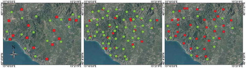
shows the location of the GGCPs (left panel) and the MGCPs (central and right panel) used for georeferencing the stereo-image with the Toutin rigorous mathematical model (left and central panel) and with the RPF model (right panel); the GCPs are marked with a red circle and the CPs with a green one.
Figure 3. Control points on the stereo-pair. Left panel: GGCPs used for rigorous math model georeferencing (both by Geomatica and SOCET); central panel: MGCPs used for rigorous math model georeferencing (by Geomatica); right panel: MGCPs used for RPF model georeferencing (by Geomatica). GCPs are marked by green circles and CPs by red squares. DATUM is ETRS89, frame ETRF00.
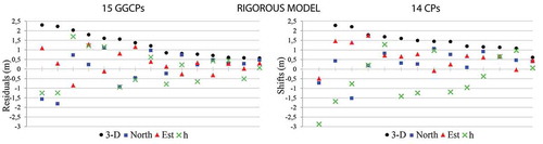
The georeferencing results using Geomatica are plotted in , the first column showing the values of the residuals on the GCPs ranked in descending order by absolute value, the second column showing the shift values on the CPs, with the same sort order.
Figure 4. Geomatica georeferencing results. Left panels: residuals on the GCPs; right panel: shift on the CPs. Top panels: Toutin rigorous model using GGCPs; central panels: rigorous model using MGCPs; bottom panels: RPF model using MGCPs.
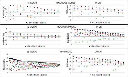
Using the rigorous mathematical model, the resulting RMSE is 0.31 m in X and 0.55 m in Y. The GCP residuals and CP shift values are lower than 1 m (in all three components) if either GGCPs or MGCPs are used, and almost the same using the RPF model (RMSE of 0.47 in X and 0.56 in Y).
The residuals and shifts from Socet Set are plotted in . Both the rigorous simultaneous model and the GGCPs have been used. The resulting RMSE in X, Y, Z is, respectively, 0.71, 0.87, 1.51 m. These values are about twice (on the same points) those obtained from Geomatica, also for the elevations.
Figure 5. Socet Set georeferencing results (rigorous simultaneous math model) obtained using GGCPs. Left panels: residuals on the GGCPs; right panel: shift on the CPs.
When the RPF model and MGCPs were used, Geomatica gave results, in terms of residual values on GCPs and shifts on CPs, of the same order of magnitude as those achieved using both the rigorous model and the GGCPs. The greater accuracy obtained on the latter points would not seem to produce a significant improvement in fitting.
The uncertainty of GPS positioning (presumably better than 10 cm) is lower than the image resolution whereas that of the points measured on the map is slightly higher. Furthermore, the NRTK GPS technique is recommended due to the speed of execution and the absence of post-processing.
In the lack of NRTK coverage, we suggest the RTK method even if the large area involved would require more master stations.
DEM extraction
In this section, we will analyze only DEMs coming from images that have been georeferenced using rigorous mathematical models and GGCPs at three different levels of resolution: 0.5, 1 and 2 m.
The score channels representing the correlation score for each DEM pixel at 1 and 2 m resolution level, setting “extra high” as the level of detail, are shown in the top panels of . The same figure (central panels) shows the corresponding cumulative frequency distribution histograms of the correlation score in percentage terms.
Figure 6. Results by Geomatica using Toutin rigorous mathematical model. Left panels: 1-m resolution DEM; right panels: 2-m resolution DEM. Top panels: score channels representing the correlation score for each DEM pixel; central panels: frequency histograms of matching correlation score; bottom panels: comparison between the coordinates of the GGCPs and stereoscopically on the epipolar images.
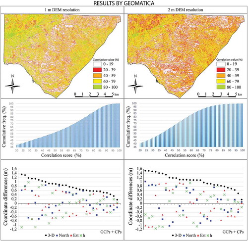
It is clear that correlation failed in most of the mountainous districts with shadowed slopes; the white areas are those where the correlation score is less than 20%, i.e. an unsuccessful correlation. These areas cover a wide portion of the image, slightly lower than 40%, for both resolutions. In the remaining portion of the image, the correlation score improves with a 1-m resolution DEM, as the greater extent of green areas in the score channel image shows as well as the corresponding histogram.
It is also possible to make a spot check of the DEM accuracy by calculating the elevation differences between the elevation values extracted from the DEM and the true values measured on the earth’s surface. The coordinates of 29 points – measured directly in stereoscopy on epipolar images – have been compared with those measured on the terrain. (bottom panels) shows a graph of the comparisons. The coordinate differences are less than 1 m for most of the points.
We also carried out this type of test on the two DEMs with spatial resolution of 1 and 2 m elaborated using Socet Set. These come from the stereo pair georeferenced using the same GGCPs used by Geomatica. shows the FOM values generated for both 1 and 2 m resolution DEMs and the corresponding frequency histograms of the correlation score in percentage values (respectively in the top and central panels).
Figure 7. Results by Socet Set using rigorous simultaneous mathematical model. Left panels: 1-m resolution DEM; right panels: 2-m resolution DEM. Top panels: FOM representing the correlation score for each DEM pixel; central panels: frequency histograms of FOM; bottom panels: comparison between the coordinates of the GGCPs and on the orthophotos.
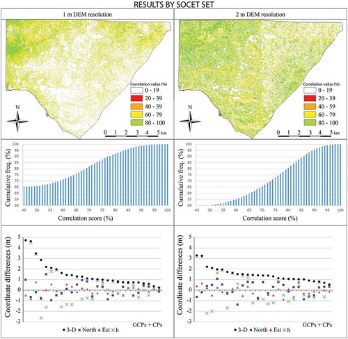
Socet Set gives a very high density of areas where the pixel correlation score reaches a value under 45 (white areas in ): 65% using a 1-m resolution DEM and 50% using a 2-m resolution one.
Where the correlation was successful, the result is therefore very good, especially for the DEM with the lower resolution (2 m).
A comparison between the coordinate values of a number of points measured on the orthophoto and of the corresponding GGCPs has also been made with SocetSet (, bottom panels). In this case, the comparison gave similar results (residuals of about 1 m) than those obtained by Geomatica, whereas the differences in elevation are much higher on a number of points when 1-m resolution DEM is used and is greater than 2 m for very few points when 2 m DEM is used.
DEM and contour maps
Contour lines are among the most important products generated by DEMs. Contour maps allow an altimetric description of the terrain surface that is crucial for subsequent geomorphological analysis. Furthermore, DEMs obtained from high-resolution imagery allow a detailed description of even small areas.
The trend of the contour lines and their readability are related more to the step of the DEM from which they are extracted than their equidistance, irrespective of the good numerical results provided by a comparison of the coordinates.
Contour lines extracted from DEMs with different resolutions produced using both software packages have been analyzed over a few subareas, highlighted in . The outputs are now analyzed from a “visual” point of view, focusing on their interpretability and looking for any problem that might arise.
Three subareas with different morphology have been chosen: a mountainous, a hilly, a flat area and the contour lines have been extracted from DEMs with three different resolution levels (0.5, 1 and 2 m).
shows the contour line maps with an interdistance of 5 m extracted using Geomatica; these contours are overlapped on correlation score maps (lines 1–3). The columns show, from left to right, the 0.5-, 1- and 2-m resolution DEMs. The images of the first lines refer to the mountainous area, those of the second lines refer to the hilly area and third lines to the flat one. In the mountainous area, the highest resolution DEM yields a good correlation score, although the real shape of the terrain surface is unsatisfactory: the contour lines are not realistic.
Figure 8. Contour lines with interdistance of 5 m on the three testing areas A, B and C. In the columns are shown, from left to right, the DEMs with a resolution of 0.5, 1 and 2 m. Contour lines are overlapped on the correlation score maps (lines 1–3) by Geomatica and on the FOM maps by Socet Set (lines 4–6).
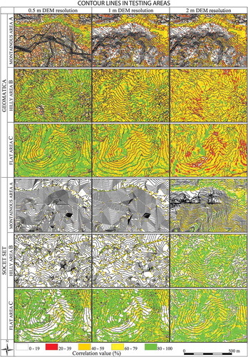
Conversely, if the low-resolution DEM (2 m) is used, some correlation difficulties highlighted in white arise: the DEM produces contour lines that appear very regular but also smooth and unreliable. In the hilly area, we notice the same behavior, albeit slightly less evident, with quite high correlation scores and reliable contour lines for the lowest resolution DEM. Also in the flat area, the best correlation scores are obtained when using the high-resolution DEM; in this case, the contour lines are broadly similar and plausible for all resolutions.
The results of these visual tests and those on numerical accuracy indicate just how important the choice of the elaboration parameters is, and they show us that the outputs used for subsequent geomorphometrical analysis should be carefully checked from various points of view.
We performed the same visual tests on the DEMs extracted by Socet Set on the test areas previously listed. As with Geomatica, the contour lines and FOMs for the three areas and for the three resolutions have been analyzed. These results are shown in .
The results we obtained in the mountainous area are not acceptable for both the highest and the medium resolution DEMs, whereas in case of the lowest resolution (2 m) for the areas with low FOM values (marked in white in the figure), the contour lines extracted are clearly unacceptable. In areas where the correlation scores are higher, they become significantly better. In the hilly area, only the lowest resolution DEM yields high correlation scores and produces acceptable contour lines. In the flat area, good results have been obtained even for the low resolution.
At a glance, Socet set produced both reliable and trustworthy contour lines if a sufficiently high correlation score is obtained, whereas in the case of high-resolution DEMs, Geomatica combines good correlation scores with contour lines that are totally unreliable.
Then, we looked at a further testing area affected by a landslide compound. This area is morphologically complex and the geomorphologists, who have a thorough knowledge of its trend, have been studying its evolution for a considerable length of time. As a result, we have acquired direct feedback on the true terrain morphology. The landsliding area is marked by letter D in .
In , we compare the results from Geomatica (the first two lines) with those from Socet Set (next two lines) in terms of both correlation/FOM scores and the 5-m spaced contour maps; the results shown in the first column refer to the 0.5-m resolution DEM, those in the second columns to the 1-m resolution and those in the third column to the lowest resolution products (2 m).
Figure 9. Testing area D. Comparison between the results by Geomatica (first two lines) with those by Socet Set (next two lines) in terms of both correlation/FOM scores and contour maps spaced 5 m. In the columns are shown, from left to right, the contour lines extracted from DEMs with a resolution of 0.5, 1 and 2 m.
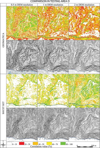
As the figure shows, for Geomatica, the 5-m spaced contour lines derived from the very high-resolution (0.5 m) DEM are highly fragmented and there are visible effects of stair steps due to the presence of man-made structures and vegetation that have not been properly removed by the filter. The result is an unacceptable DEM.
If the contour lines come from the 1-m resolution DEM, the output is better but some major stair-step effects are still present and the features of some areas do not completely match the known topography of the terrain. In order to achieve a “good” result from a visual point of view and to succeed in having regular contour lines, which are respectful of the terrain elevation, a 2-m resolution DEM should be used.
Socet SET displays a better match between the correlation score and the quality of the contour lines; both improve with a decreasing resolution of the DEM. The geomorphologists themselves, who are the final users of these products, have observed that the contour lines from Socet Set are preferable because they better match the actual profile of the terrain.
Geomorphological application
In order to analyze the surface of the terrain from a morphometric point of view, a number of feature maps extracted from the DEMs can profitably complement the contour maps (Fleming & Johnson, Citation1989; Smith, Paron, & Griffiths, Citation2011).
However, if they are to be truly useful, it is essential to carefully select the classes in which the feature values are subdivided and then visualized.
Starting from the 2-m grid DEM built with Socet Set, we have elaborated a few feature maps of slope, aspect, total curvature and terrain roughness index (TRI) on the subarea of 2.9 × 2.1 km marked with letter D in . The class division was made according to the frequency distribution of the pixel map values for the landsliding area (left bank area bordered in black on each feature map).
shows the feature maps concerning only the landsliding area.
Figure 10. Feature maps elaborated on the sub-area D, clockwise from top left: slope, aspect, terrain roughness index and total curvature. DATUM is ETRS89, frame ETRF00. The class division was made according to the frequency distribution of the values of the pixel map of the landsliding area (left bank area bordered in black on any feature map).
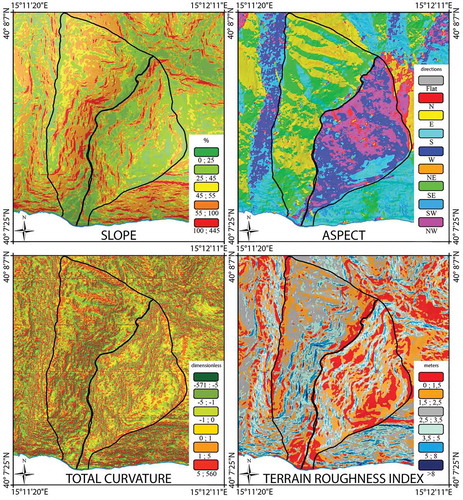
The slope map pixels have been grouped into five classes according to the five areas of the frequency distribution that have a constant trend. The slope map highlights the constant angle inclination of the right-hand side, except for some areas where the angle exceeds 45°, whereas the left-hand side has some areas with a high inclination angle value that alternate with low-value zones. The slope inclination angle increases in the area closest to the stream.
The aspect map pixels have been divided into nine classes corresponding to the cardinal directions N, NE, E, SE, S, SW, W and NW plus a class for the negative values, which indicate low-lying areas (flat). The direction is expressed in degrees, moving clockwise starting from North – which assumes the value 0.
The three types of curvature – planar, profile and tangential (total) – were computed using the curve that runs the second derivative of the DEM through a mask of standard size of 3 × 3. Note that in the tangential curvature map, there is evidence of terracing on the stable side (right bank), indicated by a regular alternation of valleys (colored in shades of green) and ridges (in orange-red). The northwest area of the map also clearly shows the curvature change between peaks and valleys. Conversely, on the unstable slope, peaks and valleys alternate in a much more “confused” way and different peaks of small size surrounded by hollows can be well distinguished.
Finally, three kinds of TRI maps have been elaborated, as mentioned in “Feature maps extraction” section. In the present test case, the most significant one was the Riley TRI, so we chose that one. Here too, the class division was carried out according to the frequency distribution of the values of the pixel maps computed for the function. The landsliding side is clearly distinguished from the opposite stable side.
On the basis of the maps we produced, a geomorphological interpretation that allows us to recognize the landslide bodies was made in (Guida &Siervo, Citation2010); the results are shown in .
Figure 11. Landslide bodies overlapped to the contour lines (drawn with an interval of 5 m) map. DATUM is ETRS89, frame ETRF00.
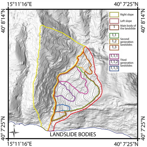
The identified landslide phenomena differ by type, age and stage of activity; so, we can distinguish between landslides of first, second and third generation. The upper part is characterized by a deformation due to a slow roto-translational motion that, running down along the sides, turns into a “strike-slip kinematics” landslide (Fleming & Johnson, Citation1989). The left and right side are characterized by a sharp break-line that lengthens into the valley. The foot of the landslide has led to an increase in slope at the front of the landslide causing both the activation of other shallow landslides and the emergence of the phenomenon known as “denutational process”.
It is possible to identify nine polygons that represent:
the right slope,
the left slope,
the main body of the landslide indicated by the abbreviation “1”,
three second generation landslides indicated by the abbreviations “1.1”, “1.2” and “1.3”,
three third generation landslides indicated by the abbreviations “1,1,1”, “1,1,2” and “1,1,3”.
We then computed some statistical indices (centrality, dispersion, asymmetry and kurtosis) for each different identified landslide with the main purpose to highlight any difference between the “right” (stable area) and the “left” (landsliding area) polygons and between the individual bodies. The “left” polygon shows similar values to some polygons contained in it and especially to “body 1” and “body 1.1”. Conversely, the statistical indices for the “body 1.3” polygon are very different from the previous ones. It is probably a different type of landslide (another generation) and it can be seen as separate from the “descendants” of “body 1”.
Discussion and conclusions
The stereo images acquired by VHR satellite sensors play an important role in cartographical and geomorphological applications, provided that all the processing steps follow strict procedures and the result of each step is carefully assessed. At the moment, there are no available shared standards. The lack of specific standards has required the study of an operational methodology that has been applied using two well-known software applications in the digital photogrammetry and remote-sensing fields.
A VHR stereo-pair satellite image has been used to reliably reconstruct the surface morphology at a high level of detail, while also allowing for the possibility of monitoring over time if subsequent images should become available.
The georeferencing phase is of utmost importance for the accuracy of the product. The number of required GCPs depends on the type of mathematical model chosen; we suggest acquiring a number of GCPs greater than that required from the software in order to employ the redundant points for a quality check.
If the rigorous model is used for georeferencing, a field survey using GPS is highly recommended. The use of NRTK services for the GCPs survey has given excellent results both for operating speed and the possibility of measuring the position of multiple neighboring points. From these, we can choose the best in terms of matching on the image.
If RPF georeferencing method is applied, a higher number of points are required; therefore, a field survey can turn out to be very time consuming. The availability of a large-scale numerical cartography has allowed us to avoid a surveying campaign as we acquired the control points directly on the map. In this case, the difficulty lies in measuring both planimetric coordinates and the height of any point with the same standard of accuracy. A few commercial codes allow a weight to be assigned to the point coordinates but, as far as we know, none allows use of solely planimetric or altimetric points.
When the rigorous model is adopted, using GCPs either surveyed on the terrain or acquired from cartography at a scale of 1:5000 has not led to major differences in the entity of residuals. We can note some differences between the two software packages: Geomatica gives georeferencing residuals under 1 m while Socet Set provides residuals on average twice that. Such a level of accuracy is achieved by using a large number of GCPs regularly spaced and well placed over the entire image.
The evaluation of the parameters with which DEMs are built is no simple task, especially as far as the choice of resolution is concerned; we have analyzed different grid steps from 0.5 m, i.e. the native spatial resolution of the image, up to four times (2 m). In order to assess both the quality and the reliability of the output, in addition to checking the values of the residuals on the control points, we have evaluated the digital matching results and the truthfulness of the extracted contour lines.
The value of the differences between the coordinates of the points directly surveyed on the field and the ones measured on the orthophotos or on the epipolar images is always lower than 2 m for the planimetric components and mostly lower than 2 m for altimetry if the 2-m resolution DEM is used. The residual amount was slightly smaller for Geomatica than for Socet Set.
With regard to the matching process, Socet Set has given higher correlation scores than Geomatica, where the lack of correlation has leaded to an uncertainty of the resulting model that does not correspond to the actual topography of the terrain.
We also notice a more reliable trend of the contour lines extracted from DEM by Socet Set. We think that a careful evaluation of the successful match of the elevation model to the real trend of the terrain is an essential point in the process, even if both the check of the residuals on control points and the digital matching are positive.
Therefore, the visual inspection of contour lines generated by the DEM – at least on some subareas – is a critical step in the process, especially if the DEM should be used to analyze the land surface morphology.
On a landsliding slope of special interest, in addition to the contour maps, we have produced a few features maps based on the DEMs. These products have allowed the geomorphologists to draw boundaries and determine the age of the various bodies in the landslide. In order to define the classes into which feature values are divided, we have taken into account the frequency histograms of the numerical values of the features.
Among the various TRIs we have tested, the one proposed by Riley turned out to be the most suitable for the geomorphological analysis of our test case.
In conclusion, we can say that the extraction of a highly accurate DEMs from high-resolution satellite stereopairs is a winnable challenge. Further studies will be needed on planned satellite images with increasing radiometric resolution in order to define standardized procedures.
Acknowledgments
We would like to thank Prof. Domenico Guida for the scientific support given in the delineation of the landslide bodies.
Disclosure statement
No potential conflict of interest was reported by the authors.
References
- Agugiaro, G., Poli, D., & Remondino, F. (2012). Testfield Trento: Geometric evaluation of very high-resolution satellite imagery. In International Archives of Photogrammetry, Remote Sensing and Spatial Information Sciences; XXII ISPRS Congress. Melbourne, Australia, Vol. 39, pp. 191–196.
- Aguilar, M.A., Del Mar Saldaña, M., & Aguilar, F.J. (2013). Assessing geometric accuracy of the orthorectification process from GeoEye-1and WorldView-2 panchromatic images. International Journal of Applied Earth Observation and Geoinformation, 21, 427–435. doi:10.1016/j.jag.2012.06.004
- Aguilar, M.A., Del Mar Saldaña, M., & Aguilar, F.J. (2014). Generation and quality assessment of stereo-extracted DSM from GeoEye-1 and Worldview-2 imagery. IEEE Transactions on Geoscience and Remote Sensing, 52(2), 1259–1271. doi:10.1109/TGRS.2013.2249521
- BAE Systems. (2007). Next-Generation Automatic Terrain Extraction (NGATE): Innovation in the cost-effective derivation of elevation data from imagery. London, UK: White Paper.
- Barbarella, M., Fiani, M., & Lugli, A. (2015). Landslide monitoring using multitemporal terrestrial laser scanning for ground displacement analysis. Geomatics, Natural Hazards and Risk, 6(5–7), 398–418. doi:10.1080/19475705.2013.8638
- Barbarella, M., Fiani, M., & Lugli, A. (2017). Uncertainty in terrestrial laser scanner surveys of landslides. Remote Sens, 9(2), 113. open access. doi:10.3390/rs9020113.
- Berry, J.K. (2013). Beyond mapping III: Procedures and applications in GIS modeling (pp. 2013). Fort Collins, Colorado: Berry & Associates, Basis Press.
- Burrough, P.A., & McDonnell, R.A. (1998). Principles of geographic information systems (2nd ed.). Oxford; New York: OUP Oxford. 2Rev Ed edition.
- Calcaterra, D., Guida, D., Budetta, P., De Vita, P., Di Martire, D., & Aloia, A. (2014). Moving geosites: how landslides can become focal points in geoparks. Latest trends in engineering mechanics, structures, engineering geology. Procedings of the 7th International Conference on Engineering mechanics, Structure, Engineering Geology (EMESEG’ 14), June 3-5, 2014; Salerno. Retrieved July 14, 2016 from http://www.wseas.us/elibrary/conferences/2014/Salerno/GEOMENG/GEOMEG-21.pdf
- Capaldo, P., Crespi, M., Fratarcangeli, F., Nascetti, A., & Pieralice, F. (2012). DSM generation from high-resolution imagery: Applications with worldview-1 and Geoeye-1. European Journal of Remote Sensing, 44, 41–53.
- Chacón, J., & Corominas, J. (2003). Special issue on landslides and gis. Natural hazards (Vol. 30:3, pp. 263–512). The Netherlands: Kluwer Academic Publishers.
- Cooley, S.W. (2015). GIS4Geomorphology. October 25, 2016. Retrieved from http://www.gis4geomorphology.com
- Liakopoulos, I., & Stanis, I. (2013). GEOEYE-1 satellite stereo-pair dem extraction using scale-invariant feature transform on a parallel processing platform (Vol. 15, pp. EGU2013).
- De Vita, P., Carratù, M.T., La Barbera, G., & Santoro, S. (2013). Kinematics and geological constraints of the slow-moving Pisciotta rock slide (southern Italy). Geomorphology, 201, 415–429. doi:10.1016/j.geomorph.2013.07.015
- Deilami, K., & Hashim, M. (2011). Very high-resolution optical satellites for DEM generation: A review. European Journal of Scientific Research, 49, 542–554.
- Dolloff, J., & Settergren, R. (2010). An assessment of worldview-1 positional accuracy based on fifty contiguous stereo pairs of imagery. Photogrammetric Engineering & Remote Sensing, 76, 935–943. doi:10.14358/PERS.76.8.935
- Drăguţ, L., & Eisank, C. (2011). Object representations at multiple scales from digital elevation models. Geomorphology, 129, 183–189. doi:10.1016/j.geomorph.2011.03.003
- Dramis, F. (2009). Editorial: geomorphological mapping for a sustainable development. Journal of Maps, 5, 53–55. doi:10.4113/jom.2009.1084.
- Esri, A.D. (2011). Documentation Manual. Redlands, CA: Environmental Systems Research Institute. Release 10.
- Evans, I.S. (1980). An integrated system of terrain analysis and slope mapping. Zeitschrift für Geomorphologie, Supplement band 36, 274–295.
- Evans, I.S., & Chorley, R.J. (1972). General geomorphometry, derivatives of altitude, and descriptive statistics. Harper & Row.
- Fleming, R.W., & Johnson, A.M. (1989). Structures associated with strike-slip faults that bound landslide elements. Engineering Geology, 27, 39–114. doi:10.1016/0013-7952(89)90031-8
- Fraser, C., & Ravanbakhsh, M. (2009). Georeferencing performance of geoeye-1. Photogrammetric Engineering & Remote Sensing, 75, 634–638.
- Gómez-Candón, D., López-Granados, F., Caballero-Novella, J.J., Peña-Barragán, J.M., & García-Torres, L. (2012). Understanding the errors in input prescription maps based on high spatial resolution remote sensing images. Precision Agricultural, 13, 581–593. doi:10.1007/s11119-012-9270-9
- Grodecki, J., & Dial, G. (2003). Block adjustment of high-resolution satellite images described by rational polynomials. Photogrammetric Engineering & Remote Sensing, 69, 59–68. doi:10.14358/PERS.69.1.59
- Guarnieri, A., Masiero, A., Vettore, A., & Pirotti, F. (2015). Evaluation of the dynamic processes of a landslide with laser scanners and Bayesian methods. Geomatics, Natural Hazards and Risk, 1, 1–21.
- Guida, D., & Siervo, V. (2010). Seminar on Landslides in Structurally Complex Formations, Unpublished manuscript. Geologist Regional Association. Salerno, Italy.
- Hanley, H.B., Yamakawa, T., & Fraser, C.S. (2002). Sensor orientation for high-resolution satellite imagery. International Archives of Photogrammetry Remote Sensing and Spatial Information Sciences, 34, 69–75.
- Hengl, T., & Reuter, H.I. (2008). Geomorphometry: Concepts, software, applications. In Developments in soil science: Vol. 33) Elsevier.
- Horn, B.K.P. (1981). Hill shading and the reflectance map. Proceedings of the IEEE, 69, 14–47. doi:10.1109/PROC.1981.11918
- Hu, X., Cheng, H., Hu, Q., Li, F., & Zeng, L. (2011). Research on road survey based on GeoEye-1 stereo images. Research on Soft Science of Surveying and Mapping 1006-9712, 40-43(1), 71.
- Hu, Y., Tao, V., & Croitoru, A. (2004). Understanding the rational function model: Methods and applications. International Archives of Photogrammetry and Remote Sensing, 20, 119–124.
- Huabin, W., Gangjun, L., Weiya, X., & Gonghui, W. (2005). GIS-based landslide hazard assessment: An overview. Progress in Physical Geography, 29, 548–567. doi:10.1191/0309133305pp462ra
- Hugenholtz, C.H., Whitehead, K., Brown, O.W., Barchyn, T.E., Moorman, B.J., LeClair, A., … Hamilton, T. (2013). Geomorphological mapping with a small unmanned aircraft system (sUAS): Feature detection and accuracy assessment of a photogrammetrically-derived digital terrain model. Geomorphology, 194, 16–24. doi:10.1016/j.geomorph.2013.03.023
- Jacobsen, K. (2009). Very high-resolution satellite images - competition to aerial images. Hyderabad, India: Map World Forum GIS Development.
- Jacobsen, K. (2011). Characteristics of very high resolution optical satellites for topographic mapping. International Archives of the Photogrammetry, Remote Sensing and Spatial Information Sciences, XXXVIII-4/W19, 137–142. doi:10.5194/isprsarchives-XXXVIII-4-W19-137-2011
- Jacobsen, K. (2013). DEM generation from high resolution satellite imagery. Photogrammetrie - Fernerkundung - Geoinformation, 2013, 483–493. doi:10.1127/1432-8364/2013/0194
- Jenness, J.S. (2004). Calculating landscape surface area from digital elevation models. Wildlife Society Bulletin, 32, 829–839. doi:10.2193/0091-7648(2004)032[0829:CLSAFD]2.0.CO;2
- Leoni, G., Barchiesi, F., Catallo, F., Dramis, F., Fubelli, G., Lucifora, S., … Puglisi, C. (2009). GIS methodology to assess landslide susceptibility: application to a river catchment of central Italy. Journal of Maps, 5, 87–93. doi:10.4113/jom.2009.1041
- Lewis, J.P. (1995). Fast template matching. Vision Interface. Vol 95 N° 120123, 15-19).
- Li, Z., Zhu, Q., & Gold, G. (2005). Digital terrain modeling: Principles and methodology. Boca Raton, Florida: CRC Press.
- Lu, P., Stumpf, A., Kerle, N., & Casagli, N. (2011). Object-oriented change detection for landslide rapid mapping. IEEE Geoscience and Remote Sensing Letters, 8, 701–705. doi:10.1109/LGRS.2010.2101045
- Meguro, Y., & Fraser, C.S. (2010). Georeferencing accuracy of GeoEye-1 stereo imagery: Experiences in a Japanese test field. International Archives of the Photogrammetry, Remote Sensing and Spatial Information Science, 38, 1069–1072.
- Murillo-García, F.G., Alcántara-Ayala, I., Ardizzone, F., Cardinali, M., Fiourucci, F., & Guzzetti, F. (2015). Satellite stereoscopic pair images of very high resolution: A step forward for the development of landslide inventories. Landslides, 12, 277–291. doi:10.1007/s10346-014-0473-1
- Niethammer, U., James, M.R., Rothmund, S., Travelletti, J., & Joswig, M. (2012). UAV-based remote sensing of the super-sauze landslide: Evaluation and results. Engineering Geology, 128, 2–11. doi:10.1016/j.enggeo.2011.03.012
- PCI Geomatics (2010). Geomatica orthoengine user guide, version 10.3. Ontario, Richmond Hill, Canada.
- Pepe, M., & Prezioso, G. (2015). A matlab geodetic software for processing airborne LIDAR bathymetry data. ISPRS-International Archives of the Photogrammetry, Remote Sensing and Spatial Information Sciences, 1, 167–170. doi:10.5194/isprsarchives-XL-5-W5-167-2015
- Poli, D., & Caravaggi, I. (2016). 3D modeling of large urban areas with stereo VHR satellite imagery: Lessons learned. Natural Hazards, 68(1), 53–78. doi:10.1007/s11069-013-0583-4
- Poli, D., & Toutin, T. (2012). Review of developments in geometric modelling for high-resolution satellite pushbroom sensors. The Photogrammetric Record, 27, 58–73. doi:10.1111/phor.2012.27.issue-137
- Riley, S., Degloria, S., & Elliot, R. (1999). A terrain ruggedness index that quantifies topographic heterogeneity. Intermountain Journal of Sciences, 5, 23–27.
- Ruszkiczay-Rüdiger, Z., Fodor, L., Horváth, E., & Telbisz, T. (2009). Discrimination of fluvial, eolian and neotectonic features in a low hilly landscape: A DEM-based morphotectonic analysis in the central Pannonian Basin, Hungary. Geomorphology, 104, 203–217. doi:10.1016/j.geomorph.2008.08.014
- Saldaña, M.M., Aguilar, M.A., Aguilar, F.J., & Fernández, I. (2012). Dsm extraction and evaluation from GEOEYE-1 stereo imagery. ISPRS Annals of Photogrammetry, Remote Sensing and Spatial Information Sciences, 4, 113–118. doi:10.5194/isprsannals-I-4-113-2012
- Shean, D.E., Alexandrov, O., Moratto, Z.M., Smith, B.E., Joughin, I.R., Porter, C., & Morin, P. (2016). An automated, open-source pipeline for mass production of digital elevation models (DEMs) from very-high-resolution commercial stereo satellite imagery. ISPRS Journal of Photogrammetry and Remote Sensing, 116(2016), 101–117. doi:10.1016/j.isprsjprs.2016.03.012
- Smith, M.J., Paron, P., & Griffiths, J.S. (2011). Geomorphological mapping: Methods and applications. Elsevier.
- Toutin, T. (2004). Review article: Geometric processing of remote sensing images: Models, algorithms and methods. International Journal of Remote Sensing, 25, 1893–1924. doi:10.1080/0143116031000101611
- Wilson, J.P., & Gallant, J.C.(Eds) (2000). Terrain analysis: principles and applications. John Wiley & Sons.
- Yaşa, F., Erbek, F.S., Ulubay, A., & Özkan, C. (2004). Geometric accuracy of high-resolution data for urban planning. XXth ISPRS. Istanbul.
- Zevenbergen, L.W., & Thorne, C.R. (1987). Quantitative analysis of land surface topography. Earth Surface Processes and Landforms, 12, 47–56. doi:10.1002/(ISSN)1096-9837
- Zhang, B. (2006). Towards a higher level of automation in softcopy photogrammetry: NGATE and LIDAR processing in SOCET SET®. GeoCue Corporation 2nd Annual Technical Exchange Conference, 26 – 27 September. Nashville, Tennessee. Unpaginated CD-ROM, 32.