Calibration of urban canopies albedo and 3D shortwave radiative budget using remote-sensing data and the DART model

ABSTRACT

The derivation of the radiative budget of urban environments has gained a high interest in the recent years as an essential part of the global energy budget of big cities. Urban 3D (three-dimensional) heterogeneity hampers its assessment with in-situ measurements, which stresses the interest of Earth Observation (EO) satellites. Improvements in remote-sensing technology and 3D urban databases open the way to new deterministic approaches. This paper presents a new method that derives maps of urban shortwave exitance, albedo and radiative budget * from EO satellite images (e.g. Sentinel 2, Landsat-8), using the discrete anisotropic radiative transfer model. In a preliminary step, it derives maps of urban material optical properties from an EO satellite image, at the spatial resolution of this EO image. The method is applied to the city of Basel, Switzerland, in the frame of the European Community H2020 URBANFLUXES (www.urbanfluxes.eu) project which aims at improving our knowledge on anthropogenic heat fluxes in European cities. Results are very encouraging. Indeed, urban * derived from 234 EO satellite images, ranging from 200 to 800 W/m² through the year, is very close to in-situ measured *: ≈15 W/m² temporal root mean square error (i.e. 2.7% mean relative difference) relative to measurements.

KEYWORDS:

• Radiative budget
• albedo
• urban canopies
• remote sensing
• DART
• 3D modelling

Introduction

Radiative budget is a major component to the urban energy budget. For any landscape, is the difference between the total incoming radiation (i.e. irradiance) and the total outgoing radiation (i.e. exitance), in every direction. A better quantification of can lead to an improved estimate of the anthropogenic heat flux . The later one is the part of the urban energy budget which is due to human activity, such as industry, traffic and house heating, among others. A good knowledge of urban is crucial for understanding fundamental processes like the contribution of anthropogenic activities to the global warming and the impact of the global warming on the urban environment on phenomena like the Urban Heat Island (Grimmond & Oke, 1999). The current study is part of the H2020 project URBANFLUXES (Chrysoulakis et al., 2015) main aim of which is to provide and share advanced methods to quantify Q_f in association with the other urban energy budget components using satellite observation from Copernicus missions and physical modelling. This objective requires the availability of time series of the urban .

is usually considered as the sum of two components: shortwave exitance mostly due to the reflexion of sun radiation in the shortwave (SW; up to 3.5 µm) spectral domain, and longwave (LW; above 3.5 µm) exitance mostly due to the urban thermal emission and to urban reflectance of atmosphere thermal emission. In this paper, we describe an innovative method for the derivation of the surface albedo and SW radiative budget of 3D (three-dimensional) urban canopies using Earth Observation (EO) satellite images, and its application to the city of Basel, Switzerland.

The determination of urban presents several difficulties (Meganem, Deliot, Briottet, Deville, & Hosseini, 2014). Indeed, it varies in time and space, mainly due to changes of urban canopy (e.g. seasonal vegetation, new buildings etc.), illumination configuration (e.g. sun direction, atmosphere condition) and urban material temperature (e.g. walls, roofs, roads). EO satellites are well adapted for detecting these changes because of their frequent observations of urban canopies with spectral bands in the SW domain. However, a major difficulty for deriving from EO is the sampling of spectral bands, incidence angles and time. For example, in the SW domain, atmospherically corrected EO satellite images correspond to information (i.e. two-dimensional [2D] radiance L_xy(→, Δλ_i)) per pixel M(x,y), for a unique solar direction Ω_s (i.e. time), a unique upward direction (i.e. sensor viewing direction) and a few spectral bands Δλ_i. Hence, this 2D spectral and directional information does not correspond to required quantities (i.e. surface albedo, exitance, ), which are double integrals over directions and spectral domain. For example, spectral exitance is a cosine weighted integral of L() over all directions of the upward hemisphere, and exitance is a sun weighted integral of spectral exitance over the sun radiation spectral domain. For each pixel, surface albedo is the ratio of its exitance and sun irradiance, and is the difference between its sun irradiance and exitance.

To transform the instantaneous and mono-directional measurements of EO satellite images into the required spatial information (i.e. maps of albedo, exitance, ), an usual approximation is to consider that the urban radiance is isotropic and consequently equal to the radiance that is measured by the EO satellite. However, this approximation does not stand for 3D urban canopies, even if urban material is lambertian. Indeed, in particular due to shadow and masking effects, a 3D landscape made of lambertian elements is not lambertian. This issue was tackled in several earlier works (Krayenhoff & Voogt, 2016, Lagouarde et al., 2010; Lagouarde & Irvine, 2008; Lagouarde et al., 2004; Voogt & Krayenhoff, 2005; Voogt & Oke, 1998). The impact of these effects, and more precisely what is actually “seen” by a satellite sensor, is for example studied by the model SUM (Soux, Voogt, & Oke, 2004). It leads to inaccurate assessment of urban , and consequently inaccurate assessment of Q_f. Here, the urban radiative anisotropy is tackled with a physically based 3D radiative transfer model that simulates accurately the mechanisms (e.g. shadow and masking effects) that explain the anisotropic behaviour of urban observations (i.e. radiance, and consequently reflectance and brightness temperature). It results that this model can simulate SW and LW observation of urban landscapes at any altitude level, including top of atmosphere. Also, it simulates the urban 3D radiative budget. The designed method is innovative. To our knowledge, there is no available method that takes advantage of 3D physical models for deriving products from EO satellite images. The few conditions to meet in order to retrieve time series from EO satellite images are indicated below:

• Availability of time series of atmospherically corrected satellite images including spectral bands that sample the spectral domain of , with a spatial resolution adapted to urban energy budget studies.

• The 3D remote-sensing model must simulate urban radiance images and radiative budget, with the consideration of the urban 3D architecture and distribution of material optical properties (OP). It implies that the model must work with the whole city and not only part of it.

• The 3D model must work with any atmospheric condition above the urban canopy and possibly air pollution in the urban canopy, which implies to simulate radiative transfer both in the atmosphere above and inside the city.

• A 3D representation of the city must be available, including a digital elevation model (DEM), and if possible vegetation location.

• A calibration method to derive maps of the urban material OP from EO satellite images. This is essential, because the urban material OP vary in time and space (e.g. tile roofs). The 3D model uses these OP (i.e. reflectance) for deriving from EO satellite images. The calibration method must be robust in order to handle all sources of inaccuracy. For example, the atmosphere correction of satellite images is never exact. Similarly, urban 3D models are never fully up to date, with the construction of new buildings, vegetation changes and so on.

In short, the objective of our work was to develop a method that computes maps of OP of urban material, and consequently maps of urban SW radiative budget using only EO data, an urban 3D representation, irradiance measured at a local flux tower and a 3D radiative transfer model. The expected spatial resolution of OP and maps is close to that of the available satellite image. In addition, irradiance and exitance values measured at a local flux tower are used to validate the method. In the URBANFLUXES project, the maps are used to get the full radiative budget maps and consequently the full urban heat balance, which leads to maps of anthropogenic heat flux . Urban 3D representations are usually derived from airborne LiDAR and imaging systems (e.g. www.teledyneoptech.com). depends a lot on the OP of the urban materials that make up the roofs, ground, vegetation etc. Unfortunately, the spatial distribution of these OP is nearly never available, which stresses the interest of the developed method, which retrieves the properties by an iterative comparison of simulated and actual EO images. In addition, the availability of this spatial distribution of urban material OP allows one to compute maps at any date (e.g. from morning to evening) as long as OP remain constant. The change of OP over time is tackled by applying the method to a new satellite image. As an expected limitation, the accuracy of the method depends on its input parameters, and particularly the atmospherically corrected EO images. The accuracy of the urban 3D representation plays also a lesser role. Indeed, an urban element that is simulated with an inaccurate geometry can nevertheless lead to an exact satellite signal because in that case the method determines OP that are either over or under estimates of the actual OP and compensate those inaccuracies. The area covered by the method depends not only on the data but also the computer power available, as well as the efficiency of the model used, as it requires to simulate the radiative transfer accurately on a complex landscape iteratively.

“The DART model” section presents the 3D radiative transfer model (discrete anisotropic radiative transfer [DART]) used in this study, and how it was adapted in order to work with the newly devised calibration method. “Derivation of urban albedo and from EO satellites and DART” section presents the DART-based method that derives maps of urban material OP from atmospherically corrected EO satellite images. It also presents how these OP are used to compute time series of maps. “Application to the case-study of Basel” section presents and comments the results obtained for the city of Basel, before final concluding remarks.

The DART model

General presentation

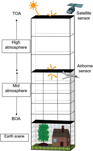
DART is a 3D radiative transfer model that tracks radiation SW and LW propagation in the Earth-atmosphere system (Gastellu-Etchegorry et al., 2015). It simulates the 3D radiative budget and the SW and LW acquisitions of imaging radiometers and LIDAR scanners aboard of space and airborne platforms, for any urban and natural landscapes (Figure 1) and any sun/sensor/atmosphere configuration (spatial and spectral resolutions, sensor viewing direction, platform altitude etc.). DART is developed at CESBIO Laboratory (www.cesbio.ups-tlse.fr/fr/dart.htm).

Figure 1. DART cell matrix of the Earth/atmosphere system. The atmosphere has three vertical levels: upper (i.e. just layers), mid (i.e. cells of any size) and lower atmosphere (i.e. same cell size as the land surface). Land surface elements are simulated as the juxtaposition of facets and turbid cells.

DART forward simulations of vegetation reflectance were successfully verified by real measurements (Gastellu-Etchegorry et al., 1999) and also cross-compared against a number of independently designed 3D reflectance models (e.g. FLIGHT [North, 1996], Sprint [Thompson & Goel, 1998], Raytran [Govaerts & Verstraete, 1998]) in the context of the RAdiation transfer Model Intercomparison experiment (Pinty et al., 2001, 2004; Widlowski et al., 2013, 2008, 2007). To date, DART has been successfully employed in various scientific applications, including development of inversion techniques for airborne and satellite reflectance images (Banskota et al., 2015, 2013; Gascon, Gastellu-Etchegorry, Lefevre-Fonollosa, & Dufrene, 2004), simulation of airborne sensor images of vegetation and urban landscapes (Yin, Lauret, & Gastellu-Etchegorry, 2015), design of satellite sensors [e.g. NASA DESDynl, CNES Pleiades, CNES LIDAR mission project (Durrieu et al., 2013)], impact studies of canopy structure on satellite image texture (Bruniquel-Pinel & Gastellu-Etchegorry, 1998), modelling of 3D distribution of photosynthesis and primary production rates in vegetation canopies (Guillevic & Gastellu-Etchegorry, 1999), investigation of influence of Norway spruce forest structure and woody elements on canopy reflectance (Malenovsky et al., 2008), design of a new chlorophyll estimating vegetation index for a conifer forest canopy (Malenovský et al., 2013) and studies of tropical forest texture (Barbier, Couteron, Gastelly-Etchegorry, & Proisy, 2012; Barbier, Couteron, Proisy, Malhi, & Gastellu-Etchegorry, 2010; Proisy et al., 2011), among others.

DART creates and manages 3D landscapes independently from the RT modelling. The major scene elements used in our study are urban buildings, ground (DEM), trees and water bodies. The term “ground” refers to surface elements such as ground, roads and grass. Trees with different geometric and OP can be exactly located within the simulated scene. In this study, vegetation was simulated as a 3D turbid medium, which corresponds to a volume of infinitely small flat surfaces that are defined by their orientation, i.e. leaf angle distribution (sr⁻¹), volume density (m²/m³) and OP of lambertian and/or specular nature. Here, tree characteristics (i.e. dimensions, geographical coordinates, leaf volume density, OP) are from external sources and/or databases (e.g. urban and vegetation OP). Urban objects (houses, roads etc.) contain solid walls and a roof built from facets defined by their orientation in space, area and OP. Finally, water bodies (rivers, lakes etc.) are simulated as facets with appropriate OP. DART can import DEMs and also urban element and urban canopy that are simulated by any software. Importantly, the imported and DART-created landscape objects can be combined to simulate Earth scenes of varying complexity. The data for the DEM, buildings and vegetation location used in this study were provided by collaborators of the URBANFLUXES project.

DART also simulates the SW and LW radiative transfer in the atmosphere for any gas and aerosols content and spectral properties (i.e. phase functions, vertical profiles, extinction coefficients, spherical albedo etc.). These quantities can be predefined manually or taken from an atmospheric database. The Earth-atmosphere radiative coupling (i.e. radiation that is emitted and/or scattered by the Earth and that is backscattered by the atmosphere towards the Earth) is simulated. It was successfully cross-compared with simulations of the MODTRAN atmosphere RT model (Gascon, Gastellu-Etchegorry, & Lefevre, 2001; Grau & Gastellu-Etchegorry, 2013).

Adaptation of the DART model for the retrieval of 3D OP

In the frame of this study, several features were added to DART in order to make it compatible with the designed method (cf. “Derivation of urban albedo and from EO satellites and DART” section).

Images per type of scene element

DART was improved in order to simulate radiance images per type n of element present in the scene (e.g. roofs, ground, vegetation etc.), in addition to the standard images , for each spectral band . One can note that a standard radiance image is the sum of all the radiance images per scene element. In addition, DART also computes cross-section images .

Spatial variability of OP

In previous DART versions, a number N of OP were defined and these OP were applied to the different scene elements. This approach can be acceptable if there is no information on the spatial variability of the urban material OP. However, in this work, EO satellites provide information about the spatial variability of the OP of scene elements. In that case, the use of this approach would lead to a number of predefined OP that would have the same order of magnitude as the number of pixels in the EO satellite image at hand, which is unacceptable. Hence, DART was improved in order to handle OP that can have any spatial variability. This improvement was applied to any spectral domain, including the VIS/NIR/SWIR and thermal infrared domains, and to all types of surface OP that are currently handled by DART: lambertian reflectance, Hapke reflectance, RPV reflectance, and also fluid OP and turbid vegetation reflectance and transmittance. In short, for any scattering or thermal emission mechanism that occurs in voxel (x, y, z), the OP of the considered scene element are multiplied by coefficients of a specific 3D matrix which size corresponds to the number of voxels of the scene. Here, a simplified method is used: all xy planes of the 3D matrix are identical.

Derivation of urban albedo and from EO satellites and DART

Introduction and materials

The implemented method aims to derive accurate albedo, exitance and maps from EO satellite images. It assesses iteratively the OP of urban materials present in the studied urban landscape and uses them to simulate the and its components. It is devised to work with any urban landscape and satellite images with any spatial resolution. Here, it is applied to the city of Basel in Switzerland, using Sentinel-2 images (it was also successfully applied with Landsat-8 images to Heraklion and part of London) and the following information:

• 3D urban model (*.obj format), with a distinction between walls and roofs, and tree information (position, dimension). It was provided by the Basel University in the frame of the URBANFLUXES project. One must note that the vegetation, wall, roof and street OP are unknown although they are required.

• Atmospherically corrected EO satellite multispectral images. Here, these images are from Sentinel-2 (20 m spatial resolution). They were atmospherically corrected by DLR (Germany) with the SEN2COR (http://step.esa.int/main/third-party-plugins-2/sen2cor/) atmosphere model. Actually, a single satellite image is enough to retrieve OP. Then, DART can use those properties for dates close to the image acquisition date. Several images are useful for taking into account the time variability of OP.

• Atmosphere and meteorological information such as bottom of atmosphere (BOA) irradiance (obtained from flux tower measurements in the city).

Figure 2 shows nadir and oblique displays of the Basel 3D database in the DART graphic user interface. Figure 3 illustrates DART-simulated images of Basel. It shows a pushbroom image (a) and a camera image (b). Both are colour composites (RGB) simulated with a 50-cm resolution, and from arbitrary sensors defined with the initial parameters from DART. They can be defined to fit the specification (e.g. FOV, spatial resolution, viewing angle) from any sensor.

Figure 2. 3D views of the DART-simulated Basel city: nadir view (left) and oblique view (right). Buildings are from the urban database. Ground and river are from the local DEM. Trees are DART created using tree locations and dimensions.

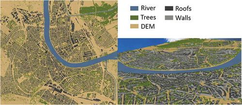
Figure 3. DART-simulated images of Basel at 50 cm resolution, with optical properties taken from the DART database. (a) Pushbroom image with zoom. (b) Camera image.

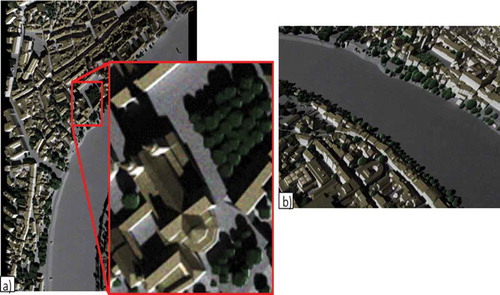
In these simulations, roofs and walls have different reflectance values (i.e. colours) that depend on their material OP and on their orientation with respect to the sun direction. However, in this simulation, material OP are spatially constant, which is most probably erroneous. This stresses the necessity to assess their spatial variability using EO satellite images. The designed method, also called “DART calibration method”, that computes these OP from EO satellite images is presented below.

Iterative DART calibration using EO satellite images

The designed method derives a map of OP per urban element from an EO satellite image, at the spatial resolution of the satellite image. In a first step, these OP are computed per pixel or group of pixels of the EO image. Indeed, if the scene elements that contribute to a given satellite pixel belong to N types of scene elements, then the consideration of a unique pixel in the satellite image leads to a single equation with N unknowns, per satellite spectral band. The adopted solution is to consider simultaneously several neighbouring pixels, with the assumption that in this group of pixels, all urban elements of the same type have the same optical property. Then, for each group of pixels, we get a system with a number of equations equal or larger than the number of unknowns. This approach leads to first-order solutions for OP: satellite and DART radiance images would be equal if urban multiple scattering was negligible compared to first-order scattering. Schematically speaking, first-order radiance is the product of the local surface reflectance ρ and sun/atmosphere irradiance. Actually, at higher scattering orders, surface irradiance depends on neighbour surface radiance, and consequently on neighbour surface reflectance and irradiance. It results that multiple order radiance tends to be proportional to powers of surface reflectance ρ (i.e. ρ², ρ³,…). Also, the situation is more complex because all neighbour surfaces do not have the same irradiance and reflectance values. Hence, after a first-order assessment of ρ, an iterative method is used to better assess the actual surface optical property such that DART and EO radiance images are nearly equal. The iterative method is an adaptation of the Newton and bisection methods. This two-step method is presented below, with N being the number of types of scene elements in the city.

Step 1.a. DART simulates two types of radiance images: scene radiance image and radiance image per scene element n, for the satellite viewing direction . The reflectance of an element n in a DART pixel , viewed along , is .

Two situations can occur

• is unknown: it is set to a plausible and spatially constant value.

• is known (e.g. from ground measurements or application of the calibration method to a previous EO satellite image): it is used as is.

The mean irradiance of scene elements of type n in DART pixel d is

(1)

where is the zenith angle of the satellite viewing direction and is the cross section of the element of type n, which is viewed by the DART pixel d along the satellite viewing direction . DART computes . The ratio had to be introduced because the radiance of any DART pixel is simulated per effective square meter of the pixel area , whereas the radiance of any element n is expressed per effective square meter of the area of the surface element itself . It can be noted that these two radiance values are equal, if and only if the considered pixel corresponds to a single element.

Step 1.b. DART scene and element radiance images are resampled down to the satellite image spatial resolution . Indeed, DART simulations are usually achieved with a finer resolution than satellite spatial resolution. Let us consider the simple case where a satellite pixel m corresponds to an integer number of DART pixels, with d the index of the DART pixels () and n the index of the type of scene element (). Then, we can define the following DART quantities at the satellite spatial resolution:

• Radiance:

(2)

• Radiance of scene element n:

(3)

• Irradiance of elements of type n:

(4)

• Cross section of element n viewed by pixel m along satellite viewing direction:

(5)

For a first approximation, Equation (4) can be written similarly as Equation (1):

(6)

In this expression, is the reflectance of scene element n in satellite pixel m, used by DART at the start of step 1. All urban elements of type n have the same reflectance in all DART pixels of satellite pixel m.

Step 1.c. DART and satellite radiance images are compared

If the for all pixels, the procedure is stopped. Otherwise, new reflectance is determined for next DART run. For that, the DART and satellite radiance images are iteratively compared, using groups of satellite pixels of increasing mesh size, starting with 1 × 1 mesh size for processing pure pixels (i.e. pixels containing only one type of urban element), and ending with a mesh size such that , in order to ensure that the resulting system has a solution. This allows to be as precise as possible when satellite pixels are not too complex in terms of number of different urban elements present, and to still solve every possible case. Each cell u contains satellite pixels m, leading to a system of equations verifying if the DART image and the satellite image are equal:

(7)

Obviously, the verification is negative if the two images differ. At iteration k, the DART radiance values are computed with inaccurate approximated OP . If we define as the DART radiance value computed from , and if we consider the hypotheses that radiance values are proportional to reflectance values (Equation (6)), then we can write:

(8)

Here, urban elements are characterized by equivalent lambertian properties (e.g. surface lambertian reflectance that ensures the equality of DART and satellite radiance images). It is an approximation that could and should be corrected in the future, especially for specular surfaces such as windows. However, results of this work stress that this assumption is quite acceptable. Indeed, for Basel, the 3D architecture of the urban canopy is most probably the major source of the urban scattering (and thermal emission anisotropy). It is coherent with the fact that a 3D scene made of lambertian surfaces is not lambertian.

Equation (7) can be written as a system of equations where the unknowns (i.e. reflectance values lead to equal first-order satellite and DART radiance images

(9)

It may happen that there is no solution for one or several cells of the mesh. For example, there is no solution if a satellite pixel contains N types of scene elements and if all the other (M² − 1) pixels of the cell of the grid contain a unique and same type of scene element. In that case, the adopted solution is to add an offset to the mesh grid, or simply to increase the mesh grid up to a value such that this problem does not occur anymore for any cell of the mesh. At the end of step 1, the material OP of all surface elements, except walls, are updated per satellite pixel . This first-order assessment is improved with the iterative method of step 2.

Step 2.a. DART uses to simulate the scene and scene element radiance images for element n and satellite viewing direction . First, k = 1.

Step 2.b. A combination of bisection and Newton’s methods (defined below) applied to the satellite and last two iteration DART radiance images leads to an up-dated optical property per scene element, per satellite pixel. The directional radiance of each pixel is

(10)

In order to ensure equality between the pixel satellite and DART radiance image, the radiance of each scene element n in the considered pixel is assumed to be

(11)

Then, using and , we consider two alternatives:

• If Newton’s method is applicable (i.e. it can determine a realistic new optical property), it is applied after computing the derivative of in the considered pixel using the two last DART surface radiance values, using Equation (12):

(12)

Solving this equation for each material of the pixel gives the new .

Back to step 2.a.

• If Newton method is not applicable, a weighted dichotomy method is used:

(13)

where the sign depends on the relative position of the satellite and last two DART radiance values. Radiance is increased with sign “+” and decreased with sign “−”. Factor α_λ is spectrally variable because the importance of multiple scattering is spectrally dependant. Here, it is simply set to 0.25. It is expected that the processing of time series of EO satellite images will allow us to adapt it per spectral band and type of scene element in order to accelerate convergence.

Back to step 2.a.

The calibration method is stopped when . Then, the OP, , albedo and exitance maps are stored for the considered spectral band.

Extension to the computation of time series

DART can use the maps of material OP per type of scene element for computing for any date, provided that local illumination conditions or atmosphere conditions are known, and provided that the scene elements OP are the same than at satellite acquisition. These two conditions tend to be easily fulfilled. Indeed, flux towers provide time series of sun irradiance and atmosphere conditions, and scene elements OP tend to remain constant, at least for dates close to the satellite image acquisition. However, scene element OP change in time with vegetation change, weather events etc. In those, cases, the solution is to apply the calibration method to a new EO satellite image.

Application to the case-study of Basel

The calibration method was applied to the city of Basel, in Switzerland. It is used below to illustrate some results such as the variation of the derived material reflectance with iterations, and also time series of maps derived from Sentinel-2 images over the year of 2016 which are compared to in-situ measurements. There are seven different elements used in the case study of Basel: roofs, ground, water, vegetation, roof structures, walls and wall structures. In the 3D model of Basel, wall/roof structures are differentiated from the overall “flat” walls and roofs. Walls and wall structure were not used in the OP retrieval, as they are not seen in satellite nadir acquisitions.

Illustration of the different steps of calibration

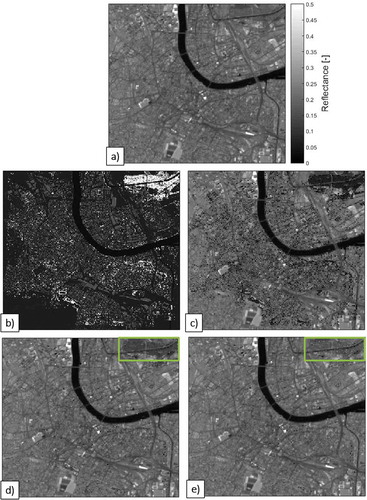
Here, the calibration method is illustrated with an atmospherically corrected Sentinel-2 image of Basel acquired on 24 June 2016, at 10:37. First, if only total BOA irradiance is available, and not direct and diffuse BOA irradiance, the DART atmosphere radiative transfer module is inverted in order to determine the atmosphere aerosol optical depth value Δτ_a such that DART-simulated BOA total irradiance matches in-situ measured total BOA irradiance (). Then, DART computes the direct sun irradiance and diffuse irradiance. Figure 4 illustrates the different steps of the method, for the band 8a of Sentinel-2 (NIR, 865 nm). It shows this Sentinel-2 image (a), and the DART image resampled to Sentinel-2 spatial resolution (i.e. 20 m) with no calibration (b), and at the end of step 1 (c), iteration 1 (d) and 2 (e). All images are reflectance images [−] with the same scale from 0 to 0.5. As expected, the DART-simulated reflectance image becomes closer to the EO satellite reflectance image, which means that the accuracy of DART simulations increases with the iteration order of the iterative calibration method. A green rectangle highlights a forest zone for which the second step of the calibration method has a very strong impact. This is explained by the fact that vegetation reflectance is very impacted by higher orders of scattering in the near-infrared region of the spectral domain.

Figure 4. Iterative calibration of DART. (a) Sentinel-2 band 8a image (20 m resolution) acquired on 24/06/2016. DART-simulated satellite reflectance image at 20 m spatial resolution without calibration (b), and at the end of step 1 (c), iteration 1 (d) and iteration 2 (e). A green box highlights a forest area in the two last iterations.

Figure 5 illustrates quantitatively how DART-simulated images become closer and closer to the Sentinel-2 image. It shows the increase in correlation happening along the calibration procedure. It compares the successive DART images with the EO acquisition, pixel per pixel at 20 m resolution. As expected, the initial comparison (top left) shows very large differences if DART is uncalibrated. The top right graph shows the improvement after the first step of calibration, the bottom left graph shows the result after 1 iteration of step 2 and the bottom right graph shows the result after a second iteration of step 2.

Figure 5. Comparison of DART and Sentinel-2 (band 8a, 865 nm; 24/06/2016) reflectance pixels at different stages of the calibration method. Top left: no calibration. Top right: end of step 1. Bottom left: first iteration. Bottom right: second iteration.

RMSE_S is the systematic RMSE. It is the root of the mean squared difference between the regressed predictions and the observations. It informs on the linear error of the regression model. RMSE_U is the unsystematic root mean square error (RMSE). It is the root of the squared difference between the predictions and the regressed predictions. It is a measure of errors due to random processes affecting the regression (Willmott, 1981; Willmott et al., 1985; Wilmott, Robeson & Matsuura, 1981). We have. Between the first non-calibrated reflectance map and the final map after the application of the calibration method, the r² coefficient between the Sentinel-2 image and the DART image increases from less than 1% up to 97% and the RMSE decreases from 0.14 down to 0.01 [−]. It is important to note that results differ between spectral bands. For example, the convergence is faster for the visible spectral bands, because multiple scattering mechanisms are usually small in these bands. To better understand this convergence, the reflectance variation was analysed per pixel (Figure 6).

Figure 6. Evolution of the DART reflectance (cross markers) of pixels that correspond to three urban surface elements (top left: pure vegetation; top right: ground; bottom: central city), compared to Sentinel-2 reflectance (circle markers) for the same pixels.

In the calibration method, DART reflectance images converge towards the Sentinel-2 reflectance images. Figure 6 illustrates this convergence at 865 nm (Sentinel-2 8a band). It must be kept in mind that at 865 nm, the convergence is the lowest due to the importance of multiple scattering mechanisms. Three pixels that correspond to three distinct urban ground covers are considered:

• Pure vegetation (top-left): the initial DART reflectance overestimates Sentinel-2 reflectance. This is simply due to the fact that the initial OP of vegetation are too large. Step 1 leads to smaller OP of vegetation which translates into a smaller DART reflectance, which underestimates the Sentinel-2 reflectance value. Step 1 does not lead to a correct reflectance value because it neglects multiple scattering events. As expected, the iterations of step 2 lead to urban element (not only vegetation) OP such that DART reflectance converges towards Sentinel-2 reflectance.

• Pure ground (top-right): the calibration method is very efficient for this ground cover. Indeed, multiple scattering is very small; it is mostly due to neighbouring areas. Hence, at the end of step 1, reflectance convergence is nearly reached.

• City-built area (bottom plot): this pixel was selected in order to illustrate that step 1 of the calibration method can give material OP that lead to DART reflectance that diverges from Sentinel-2 reflectance. This behaviour is explained by multiple scattered radiation from neighbour areas for which the calibration method gives inaccurate material OP. As expected, iterations of step 2 lead to DART reflectance that converges towards Sentinel-2 reflectance.

Results: albedo and SW radiative budget maps

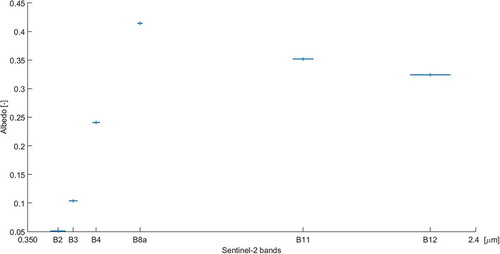
DART uses the material OP given by the calibration method for each Sentinel-2 band to compute the spectral band albedo, exitance and radiative budget maps. They are computed as an integral over the upward directions of the upper hemisphere, per Sentinel-2 band. Figure 7 shows the band albedos for a single pixel.

Figure 7. DART spectral albedo of a single pixel for Sentinel-2 bands 2, 3, 4, 8a, 11 and 12. These bands illustrate the albedo behaviour in the short wavelengths.

In a second step, the SW albedo and exitance are computed as spectral integral of the spectral albedo and exitance weighted by irradiance :

(14)

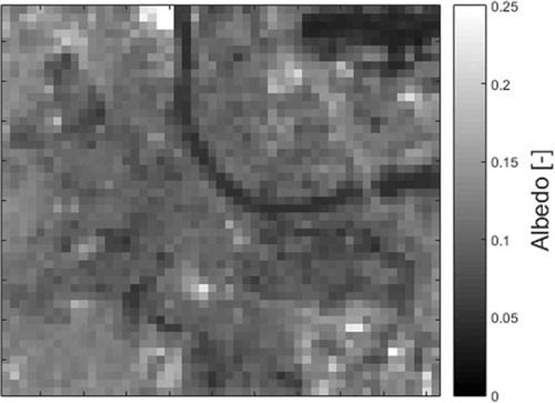
Figure 8 shows the albedo map for 24 June 2016 at 10:37. Here, it is resampled to a 100-m grid to fit the requirements of the project.

Figure 8. Basel albedo map on 24 June 2016 at 10:37. It is derived from a Seninel-2 image acquired at the same date. Spatial resolution is 100 m (URBANFLUXES grid).

SW radiative budget is the difference of SW irradiance and exitance:

(15)

It can be noted that DART simulates directly the albedo and exitance quantities. Figure 9 shows the map of 24 June 2016 at 10:37. The red dot indicates the position of the flux tower BKLI used both for calibrating SW irradiance and for testing the accuracy (cf. next section) of DART . This flux tower is an 18-m high mast atop a 20-m high building (i.e. 38 m above the ground). In Figure 9, spatial variations are coherent with our knowledge of Basel 3D structure and materials. For example, the forest area (top right) has larger values. However, we can note unusually low values in the bottom left. This is because the Basel 3D database was not available for this area, at the time of the study. Hence, this area was processed as a bare ground surface with lambertian material and topography from the available DEM. This highlights the importance of having urban 3D databases.

Figure 9. Basel map [W/m²] at 100 m resolution (URBANFLUXES grid), on 24 June 2016 at 10:37. The red dot represents the BKLI flux tower location.

Results: time series and validation

A time series of maps was produced for the year 2016, through the application of the calibration method to all available Sentinel-2 images of 2016 (Table 1). Hence, the OP of the urban materials were updated throughout 2016 using Sentinel-2 acquisitions. The most significant changes in OP occurred in the vegetated areas (e.g. fields, forests) as the phenology of the vegetation evolved with the seasons. It led to variations of urban exitance, albedo and reflectance. Urban exitance changed also with the change of shadows in relation with the change of sun direction. These changes are automatically taken into account by DART, and thus by the methodology. Some scenes were partly cloudy but still allowed to update the properties of clear areas. BKLI flux tower measurements, provided by the University of Basel, were used to calibrate the SW irradiance for assessing the accuracy of DART-simulated . In the frame of the URBANFLUXES project, MODIS acquisitions were used to get information on LW domain, for computing time series of : 122 MODIS-Terra and 112 MODIS-Aqua day scenes were processed, which lead to 234 maps of Basel. All the MODIS acquisitions were between 09:50 and 13:10. Figure 10 shows the simulated flux at the time of MODIS acquisitions and at the BKLI tower location. has a regular pattern along the year, with maximal values in early summer (≈850 W/m²) and minimal values in winter (≈300 W/m²). More scenes are available in summer because winter scenes are cloudier.

Table 1. Acquisition date, time and cloud cover of the available Sentinel-2 images in 2016.

Acquisition date	Acquisition time	Cloud status
31 December 2016	10:34:28	***
21 December 2016	10:34:34	***
01 December 2016	10:34:12	***
01 November 2016	10:32:02	–
22 October 2016	10:30:52	***
12 September 2016	10:35:51	*
02 September 2016	10:32:28	*
23 August 2016	10:33:32	–
13 August 2016	10:32:28	–
24 June 2016	10:37:21	*
25 May 2016	10:32:33	*
05 May 2016	10:30:27	–
26 March 2016	10:34:06	***
05 February 2016	10:35:56	***
26 January 2016	10:46:30	***

Cloud free (–), almost cloud free (*) and moderately cloudy (***).

Figure 10. Simulated [W/m²] at the location of the BKLI flux tower at the time of 234 MODIS acquisitions in the year 2016. Seasons are distinguished: spring (green triangles), summer (red diamonds), autumn (yellow crosses) and winter (blue circles).

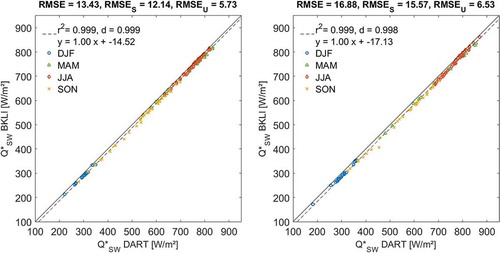
DART/EO satellite and BKLI flux tower were compared for each MODIS acquisition (Figure 11). Results are very encouraging. They show a strong correlation, high r² coefficient and a low RMSE. The mean relative difference over both time series is 2.7%. It is more or less season independent. Additionally, the assumption that OP do not vary excessively between satellite acquisitions seems to stand, since the material OP were derived from only 15 Sentinel-2 images. This assumption was further tested using OP derived from a Landsat-8 image, for the simulation of other Landsat-8 images. In that case, the relative difference was smaller than 5%. One can note a constant small bias on . Indeed, most of the RMSE comes from the systematic component of the error. We believe that it is due to the walls OP. Indeed, because walls are not seen in Sentinel-2 images, their reflectance is simply an initial reflectance value from the DART spectral database, without any possible update with EO satellite images. However, walls affect and also influence indirectly Sentinel-2 images through multiple scattering mechanisms. Results suggest that the initial wall reflectance is too low (at least in the tower area), which leads to a slightly too large DART . Hence, wall reflectance is an adjustable model parameter that could be adjusted for decreasing the systematic difference (RMSE_S). This approach would lead to a spatially constant wall reflectance. Wall reflectance spatial variation could be considered using local information about wall characteristics such as colour.

Figure 11. DART/EO satellite and BKLI flux tower for the 234 available MODIS-Terra (left) and MODIS-Aqua (right) acquisitions. Spring (green triangle), summer (red diamond), autumn (yellow cross) and winter (blue circle). Mean relative difference is 2.7% for the combined time series.

We must keep in mind that this validation, even if it uses many scenes, can only be made in one location (i.e. flux tower). Also, the 100-m resolution certainly smooths out errors. However, this spatial resolution is well adapted to the project objective.

Concluding remarks and perspectives

An innovative method for deriving accurate urban maps was designed and successfully tested for the city of Basel, Switzerland, in the frame of the H2020 URBANFLUXES project. It derives iteratively maps of SW OP per type of urban element from EO satellite images, using the 3D radiative transfer model DART and a 3D representation of the studied urban landscape. The approach relies on an iterative comparison of DART-simulated images and images of EO satellites. In a second step, DART uses these assessed OP to simulate maps of irradiance of the urban landscape, and consequently maps at any time. This method works with any atmospherically EO satellite image with any spatial resolution. For example, the method works perfectly with Landsat-8 and Sentinel-2 images, which allows one to take advantage of Sentinel-2 high revisit for updating the OP of urban elements. Also, the method is designed to work with any urban landscape, provided a 3D urban representation is available.

The calibration method was applied to Basel, Switzerland. DART images resampled to 20 m resolution were used to derive urban material OP from Sentinel-2. The resulting DART reflectance images match very well with Sentinel-2 reflectance images (mean RMSE ≈ 0.01 [−]). The availability of 15 Sentinel-2 images allowed us to update the urban element OP during the year 2016. DART used these properties for simulating a time series of maps for 234 dates in 2016. These dates correspond to 234 MODIS acquisitions. The accuracy of DART was assessed using the Basel BKLI flux tower. DART proved to be very accurate: large r² coefficient (>0.99), and small differences (RMSE ≈ 15 W/m², relative difference ≈ 2.7%) relative to BKLI flux tower . Also, they proved that a few satellite acquisitions throughout the year can lead to accurate maps. It can be noted that, compared to the total RMSE, a relatively strong systematic RMSE arises. We attributed it to the inaccurate wall reflectance used by DART. Indeed, wall reflectance cannot be derived from EO satellites because walls are not viewed from space. Overall, results are very encouraging. Work continues on the following points:

• Application of the calibration method to other test sites. It is being done for the cities of London and Heraklion (test sites of URBANFLUXES). Preliminary comparisons with London flux towers lead to similar accuracy than for Basel.

• Extension of the calibration method to LW for obtaining DART full radiative budget maps. For that, maps are first derived from multispectral thermal EO images through a similar method that achieves a simultaneous determination of the urban material emissivity and temperature. It has already been preliminary applied to Landsat-8 and ASTER EO LW satellites.

In short, the calibration method can derive accurate maps from EO satellite images, using DART model and an urban database, without the need of in-situ measurements, although the latter ones could improve results.

Depending computer facilities, computer time can be an issue for simulating times series of maps. In order not to run DART for each time step, the adopted solution, not presented here, is to pre-compute white sky albedo (i.e. albedo for sky illumination only) and black sky albedo (i.e. albedo for direct sun illumination only), for finite number of sun directions, and then to convolve these albedos with in-situ direct and diffuse irradiance values.

Disclosure statement

No potential conflict of interest was reported by the authors.

Additional information

Funding

This work was supported by EU Framework Programme for Research and Innovation H2020 [Grant Number637519], project URBANFLUXES (http://urbanfluxes.eu/).

References

- Banskota, A., Serbin, S.P., Wynne, R.H., Thomas, V.A., Falkowski, M.J., Kayastha, N., … Townsend, P.A. (2015). An LUT-based inversion of DART model to estimate forest LAI from hyperspectral data. IEEE Journal of Selected Topics in Applied Earth Observations and Remote Sensing, 8, 3147–3160.
- Banskota, A., Wynne, R.H., Thomas, V.A., Serbin, S.P., Kayastha, N., Gastellu-Etchegorry, J.P., & Townsend, P.A. (2013). Investigating the utility of wavelet transforms for inverting a 3-D radiative transfer model using hyperspectral data to retrieve forest LAI. Remote Sensing, 5(6), 2639–2659.
- Barbier, N., Couteron, P., Gastelly-Etchegorry, J.-P., & Proisy, C. (2012). Linking canopy images to forest structural parameters: Potential of a modeling framework. Annals of Forest Science, 69(2), 305–311.
- Barbier, N., Couteron, P., Proisy, C., Malhi, Y., & Gastellu-Etchegorry, J.-P. (2010). The variation of apparent crown size and canopy heterogeneity across lowland Amazonian forests. Global Ecology and Biogeography, 19(1), 72–84.
- Bruniquel-Pinel, V., & Gastellu-Etchegorry, J.P. (1998). Sensitivity of texture of high resolution images of forest to biophysical and acquisition parameters. Remote Sensing of Environment, 65(1), 61–85.
- Chrysoulakis, N., Heldens, W., Gastellu-Etchegorry, J.-P., Grimmond, S., Feigenwinter, C., Lindberg, F., … Olofson, F. (2015). Urban energy budget estimation from sentinels: The URBANFLUXES project. MUAS.
- Durrieu, S., Cherchali, S., Costeraste, J., Mondin, L., Debise, H., Chazette, P., … Pélissier, R. (2013). Preliminary studies for a vegetation ladar/lidar space mission in france. In Proceedings of the international geoscience and remote sensing symposium, IGARSS 2013, IEEE international (pp. 2332–2335). Melbourne, Australia.
- Gascon, F., Gastellu-Etchegorry, J.-P., & Lefevre, M.-J. (2001). Radiative transfer model for simulating high-resolution satellite images. IEEE Transactions on Geoscience and Remote Sensing, 39(9), 1922–1926.
- Gascon, F., Gastellu-Etchegorry, J.-P., Lefevre-Fonollosa, M.-J., & Dufrene, E. (2004). Retrieval of forest biophysical variables by inverting a 3-D radiative transfer model and using high and very high resolution imagery. International Journal of Remote Sensing, 25(24), 5601–5616.
- Gastellu-Etchegorry, J.P., Guillevic, P., Zagolski, F., Demarez, V., Trichon, V., Deering, D., & Leroy, M. (1999). Modeling BRF and radiation regime of boreal and tropical forests: I. BRF. Remote Sensing of Environment, 68(3), 281–316.
- Gastellu-Etchegorry, J.-P., Yin, T., Lauret, N., Cajgfinger, T., Gregoire, T., Grau, E., … Ristorcelli, T. (2015). Discrete anisotropic radiative transfer (DART 5) for modeling airborne and satellite spectroradiometer and LIDAR acquisitions of natural and urban landscapes. Remote Sensing, 7, 1667–1701.
- Govaerts, Y.M., & Verstraete, M.M. (1998). Raytran: A Monte Carlo ray-tracing model to compute light scattering in three-dimensional heterogeneous media. IEEE Transactions on Geoscience and Remote Sensing, 36(2), 493–505.
- Grau, E., & Gastellu-Etchegorry, J.P. (2013). Radiative transfer modeling in the Earth–Atmosphere system with DART model. Remote Sensing of Environment, 139, 149–170.
- Grimmond, C.S.B., & Oke, T.R. (1999). Heat storage in urban areas: Local-scale observations and evaluation of a simple model. Journal of Applied Meteorology, 38, 922–940.
- Guillevic, P., & Gastellu-Etchegorry, J.P. (1999). Modeling BRF and radiation regime of boreal and tropical forest: II. PAR regime. Remote Sensing of Environment, 68(3), 317–340.
- Krayenhoff, E., & Voogt, J. (2016). Daytime thermal anisotropy of urban neighbourhoods: Morphological causation. Remote Sensing, 8(2), 108.
- Lagouarde, J.-P., Hénon, A., Kurz, B., Moreau, P., Irvine, M., Voogt, J., & Mestayer, P. (2010). Modelling daytime thermal infrared directional anisotropy over Toulouse city centre. Remote Sensing of Environment, 114(1), 87–105.
- Lagouarde, J.-P., & Irvine, M. (2008). Directional anisotropy in thermal infrared measurements over Toulouse city centre during the CAPITOUL measurement campaigns: First results. Meteorology and Atmospheric Physics, 102, 173–185.
- Lagouarde, J.-P., Moreau, P., Irvine, M., Bonnefond, J.-M., Voogt, J., & Solliec, F. (2004). Airborne experimental measurements of the angular variations in surface temperature over urban areas: Case study of Marseille (France). Remote Sensing of Environment, 93(4), 443–462.
- Malenovský, Z., Homolová, L., Zurita-Milla, R., Lukeš, P., Kaplan, V., Hanuš, J., … Schaepman, M.E. (2013). Retrieval of spruce leaf chlorophyll content from airborne image data using continuum removal and radiative transfer. Remote Sensing of Environment, 131, 85–102.
- Malenovsky, Z., Martin, E., Homolova, L., Gastellu-Etchegorry, J.P., Zurita-Milla, R., Schaepman, M.E., … Cudlin, P. (2008). Influence of woody elements of a Norway spruce canopy on nadir reflectance simulated by the DART model at very high spatial resolution. Remote Sensing of Environment, 112(1), 1–18.
- Meganem, I., Deliot, P., Briottet, X., Deville, Y., & Hosseini, S. (2014, January). Linear–quadratic mixing model for reflectances in urban environments. IEEE Transactions on Geoscience and Remote Sensing, 52(1), 544–558.
- North, P. (1996). Three-dimensional forest light interaction model using a Monte Carlo method. IEEE Transactions on Geoscience and Remote Sensing, 34(4), 946–956.
- Pinty, B., Gobron, N., Widlowski, J., Gerstl, S., Verstraete, M., Antunes, M., … Thompson, R. (2001). Radiation transfer model intercomparison (RAMI) exercise. Journal of Geophysical Research: Atmospheres, 106(D11), 11937–11956.
- Pinty, B., Widlowski, J.-L., Taberner, M., Gobron, N., Verstraete, M.M., Disney, M., … Zang, H. (2004). Radiation transfer model intercomparison (RAMI) exercise: Results from the second phase. Journal of Geophysical Research: Atmospheres, 109(D6), 1–19.
- Proisy, C., Barbier, N., Guéroult, M., Pélissier, R., Gastellu-Etchegorry, J.P., Grau, E., & Couteron, P. (2011). Biomass prediction in tropical forests: The canopy grain approach. Remote Sensing of Biomass: Principles and Applications, 1–18.
- Soux, A., Voogt, J.A., & Oke, T.R. (2004). A model to calculate what a remote sensor `sees’ of an urban surface. Boundary-Layer Meteorology, 111, 109–132.
- Thompson, R.L., & Goel, N.S. (1998). Two models for rapidly calculating bidirectional reflectance of complex vegetation scenes: Photon spread (PS) model and statistical photon spread (SPS) model. Remote Sensing Reviews, 16(3), 157–207.
- Voogt, J., & Krayenhoff, E. (2005, March 14–16). Modeling urban thermal anisotropy. 5th International Symposium on Remote Sensing of Urban Areas, Phoenix, AZ.
- Voogt, J.A., & Oke, T.R. (1998). Effects of urban surface geometry on remotely-sensed surface temperature. International Journal of Remote Sensing, 19(5), 895–920.
- Widlowski, J.L., Pinty, B., Lopatka, M., Atzberger, C., Buzica, D., Chelle, M., … Xie, D. (2013). The fourth radiation transfer model intercomparison (RAMI-IV): Proficiency testing of canopy reflectance models with ISO-13528. Journal of Geophysical Research: Atmospheres, 118(13), 6869–6890.
- Widlowski, J.-L., Robustelli, M., Disney, M., Gastellu-Etchegorry, J.-P., Lavergne, T., Lewis, P., … Verstraete, M.M. (2008). The RAMI On-line Model Checker (ROMC): A web-based benchmarking facility for canopy reflectance models. Remote Sensing of Environment, 112(3), 1144–1150.
- Widlowski, J.-L., Taberner, M., Pinty, B., Bruniquel-Pinel, V., Disney, M., Fernandes, R., … Xie, D. (2007). Third radiation transfer model intercomparison (RAMI) exercise: Documenting progress in canopy reflectance models. Journal of Geophysical Research: Atmospheres, 112(D9). doi:10.1029/2006JD007821
- Willmott, C.J. (1981). On the validation of model. Physical Geography, 2(2), 184–194.
- Willmott, C.J., Ackleson, S.G., Davis, R.E., Feddema, J.J., Klink, K.M., Legates, D.R., … Rowe, C.M. (1985). Statistics for the evaluation and comparison of models. Journal of Geophysical Research, 90(C5), 8995–9005.
- Willmott, C.J., Robeson, S.M., & Matsuura, K. (1981). A refined index of model performance. International Journal of Climatology. doi:10.1002/joc.2419
- Yin, T., Lauret, N., & Gastellu-Etchegorry, J.-P. (2015). Simulating images of passive sensors with finite field of view by coupling 3-D radiative transfer model and sensor perspective projection. Remote Sensing of Environment, 162, 169–185.