The Sensitivity of Value-Added Estimates to Specification Adjustments: Evidence From School- and Teacher-Level Models in Missouri

Abstract

We provide a side-by-side comparison of school and teacher growth measures estimated from different value-added models (VAMs). We compare VAMs that differ in terms of which student and school-level (or teacher-level) control variables are included and how these controls are included. Our richest specification includes 3 years of prior test scores for students and the standard demographic controls; our sparsest specification conditions only on a single prior test score. For both schools and teachers, the correlations between VAM estimates across the different models are high by conventional standards (typically at or above 0.90). However, despite the high correlations overall, we show that the choice of which controls to include in VAMs, and how to include them, meaningfully influences school and teacher rankings based on model output. Models that are less aggressive in controlling for student-background and schooling-environment information systematically assign higher rankings to more-advantaged schools, and to individuals who teach at these schools.

KEY WORDS::

• Educational accountability
• Growth model
• School quality
• Teacher quality

1. INTRODUCTION

A large amount of research literature has emerged over the past two decades showing that important performance differences exist across schools and teachers (e.g., see Betts 1995; Hanushek and Rivkin 2010). Moreover, these performance differences are difficult to predict using observable measures of teacher qualifications and/or schooling inputs (Aaronson et al. 2007; Betts 1995; Hanushek 1996). Given the difficulty in predicting student outcomes based on measured inputs, school districts and state education agencies across the United States are increasingly interested in using outcome-based measures, including those from value-added models (VAMs), to identify effective and ineffective schools and teachers.¹

Education officials charged with selecting value-added models for use in school and/or teacher evaluations are greatly concerned with the practical implications of model specification. The objective of the present study is to provide side-by-side comparisons across a variety of VAM specifications to help inform the model-selection process.² Using administrative microdata from Missouri, we compare models that differ in terms of the number of lagged test scores and the types of other control variables that are included. We also compare the standard one-step VAM to a two-step model that partials out the influence of lagged test scores, student characteristics, and schooling-environment controls prior to estimating growth measures for schools and teachers.

Our findings are presented in a way that we hope will make it easier for educational administrators, policymakers, and other interested parties to quickly identify the tradeoffs that come with choosing different VAM specifications. We highlight two key results from our analysis. First, there are only modest benefits in model performance associated with including multiple lagged test scores in VAMs. In addition, moving from a specification with three lagged scores to one with a single lagged score does not systematically benefit or harm certain types of schools or teachers (e.g., those in primarily advantaged or disadvantaged areas). This finding suggests that the benefits associated with adding multiple lagged test scores to the model are likely to be outweighed by the cost that comes in terms of lost data. For example, in a standard VAM framework, moving from a model with one lagged score to one with two lagged scores would necessitate dropping all grade-4 students from the analysis (assuming testing starts in grade-3).³

The second key insight from our study is that which controls are included in the models, and how they are included, meaningfully shapes the groups of “winners” (top quartile) and “losers” (bottom quartile) in VAM-based evaluations. This result holds despite the fact that the correlations between estimates across all of our specifications are at or above 0.90. At one end of the spectrum are models that omit information about student background and schooling environments entirely. In these models, teachers and schools in disadvantaged areas are disproportionately represented in the bottom quartile of VAM-based rankings, while teachers and schools in advantaged areas are disproportionately represented in the top quartile. At the other end of the spectrum are our two-step models that generate “proportional” rankings for schools and teachers by construction, such that teachers and schools in advantaged and disadvantaged areas are evenly represented throughout (see Ehlert et al. 2013).

2. DATA

We estimate value-added models (VAMs) for schools and teachers using administrative microdata from middle and junior-high schools in Missouri. We use Missouri Assessment Program (MAP) scores from 2009–2010 in math and communication arts as the outcome variables in our models and standardize all student scores within subject and grade.⁴ Although we use multiple lagged test scores as controls in our models, we estimate models that use just a single year of outcome data. We elaborate on the implications of this feature of our study below.⁵

At the school-level, we use data from all middle and junior high schools in the state of Missouri that serve students in grades 6, 7, and/or 8. The following control variables are available for each student record: up to 3 years of lagged test scores, eligibility for free/reduced-price lunch, language status (whether English is a second language), special-education status, race, and gender. In some models, we also include measures of each of these control variables aggregated to the school level.

We estimate “full” models that use all three lagged test scores as predictor variables for each student, as well as models that condition on just a single lagged score. Because our analysis focuses on middle and junior-high schools, we do not encounter any issues related to structurally missing data when estimating the full models.⁶ However, some students who could potentially have a full score history do not. For example, a grade-6 student may be missing her grade-4 score. Possible solutions to this type of missing-data problem include dropping the students with missing scores (list-wise deletion) or imputation. In the present analysis, we simply drop students with incomplete score histories, which results in our dropping roughly 9% of the observations in our sample. Our decision to deal with the missing data using list-wise deletion is inconsequential to our findings and we obtain similar results if we impute the missing data instead.

Table 1. Basic descriptive statistics. School-level data

	Full model	One-test model
% Free/reduced lunch	42.5	43.3
% English as a 2nd language	1.8	2.0
% Special education	11.9	12.0
% Disadvantaged minority	19.9	20.5
% Female	49.3	49.1
Schools	348	348
Students (math)	133,773	146,938
Students (com arts)	133,535	146,896

NOTE: Disadvantaged minorities are defined as being American Indian, black or Hispanic. Student characteristics are calculated using all students who are included in either the math or communication-arts model. Some grade-6 students in Missouri attend elementary schools but most attend middle schools. Grade-6 students in middle schools are included in our analysis.

Table 1A. Basic descriptive statistics. Teacher-level data

	Full model	One-test model
% Free/reduced lunch	47.1	47.4
% English as a 2nd language	4.0	4.5
% Special education	13.6	13.5
% Disadvantaged minority	46.6	46.6
% Female	49.4	49.3
Teachers (math)	289	289
Teachers (com arts)	388	390
Students (math)	18,910	20,871
Students (com arts)	19,150	21,129

NOTE: Disadvantaged minorities are defined as being American Indian, black or Hispanic. Student characteristics are calculated using all students who are included in either the math or communication-arts model.

Our teacher-level analysis runs in parallel to our school-level analysis to facilitate comparison; therefore, much of the preceding discussion pertains to our teacher-level data as well. The primary difference between our school- and teacher-level work is that our teacher-level models do not use data from the entire state. Instead, we estimate teacher value-added using data from a cluster of 16 school districts in the St. Louis area.⁷ A second difference between the school- and teacher-level models is that the unit aggregates for the teacher-level models are computed at the classroom level.⁸

Tables 1 and 1A report basic summary statistics for our school- and teacher-level datasets, respectively. Table 1A highlights the relative disadvantage of the schools in the cluster of districts from the St. Louis area, which can be seen by comparing the descriptive statistics reported in Table 1A to those reported in Table 1. Table 1A also shows that there are more communication-arts teachers than math teachers in our analytic sample, which reflects smaller communication-arts classes.

3. EMPIRICAL APPROACH

We estimate two types of value-added models. The first is a standard one-step fixed effects model that takes the following form: (1)

In (1), is a test score for student i in year t in either math or communication arts, is a vector of observable student characteristics, and is a vector of indicator variables for either the school or teacher to which student i is assigned in year t. The vector δ represents the value-added measures (for either schools or teachers), which are estimated as fixed effects. Because we only use outcome data from a single year, the unit indicators, , also absorb the influence of all unit-level characteristics. For example, in the school-level models we cannot separately identify the school fixed effects and the effects of school-aggregated student demographics.

We also estimate two-step models, as shown in Equations (2) and (3): (2) (3)

The variables in Equations (2) and (3) that overlap with those in Equation (1) are defined similarly. The vector is also added in the two-step model. includes unit-level aggregates (school or teacher, depending on the model) of the lagged-test-score and student-covariate controls.

The key substantive feature that distinguishes the one-step and two-step models is that the two-step model partials out the variation in attributable to lagged test scores and other controls before estimating the school or teacher effects. This allows for the separate inclusion of covariates aggregated to the level of the unit of analysis (school or teacher). The practical implication of the ordering of the steps is that any differences in school or teacher performance that are systematically correlated with the covariates, at either the individual or unit-of-analysis levels, will be attributed to the covariates (and similarly for lagged test scores). Put differently, the two-step model essentially equalizes competing units based on observable student characteristics prior to comparing value-added between units.⁹

Our inability to separate out the influence of the unit-level aggregates from the unit effects themselves with a single year of data forces a clear choice about bias between models. In particular, as noted above, the one-step model potentially conflates the unit effects with other factors (e.g., school compositions). Alternatively, the two-step procedure has the potential to “overcorrect” for observable differences between units by estimating the model in sequence, as shown in Equations (2) and (3).¹⁰

The direction and magnitude of the bias in each model cannot be determined with certainty because the underlying true values of the unit effects are unknown. However, the potential bias in the one-step model likely favors advantaged schools, while the potential bias in the two-step model likely favors disadvantaged schools. For example, if having more low-SES peers lowers student test scores, then the estimated school effects from the one-step model, which cannot separately account for school compositions, will be confounded by differences in peer quality across schools.¹¹ Alternatively, if schools in disadvantaged areas have lower-quality teachers, which appears to be the case (e.g., see Sass et al. 2012), these teacher-quality differences will be purged from the residuals in the first-step of the two-step model before the school or teacher effects are estimated, which will favor schools and teachers in disadvantaged areas.

In the analysis that follows our “full” specifications are as shown in Equations (1), (2), and (3). We also consider restricted versions of each model that include different lagged test score histories and student covariates. A key objective of our study is to provide side-by-side comparisons across a variety of VAM specifications to help inform policymakers involved in the model-selection process.

Finally, we briefly note that a third modeling strategy—which we do not evaluate directly—is a one-step model that also includes unit-aggregated student characteristics. Such a model can be mechanically identified if multiple years of student test-score data are available; however, the variation used to identify the coefficients on the student and unit-level control variables occurs only within units. As noted by Ehlert et al. (2013) in their discussion of the one-step VAM, the reliance on within-unit variation for identification has the potential to be particularly problematic in the case of the unit-aggregate characteristics, which are meant to control for school and/or classroom environments. Ehlert et al. (2013) caution that mechanical identification is not a sufficient condition for obtaining the parameters of interest for the unit-level aggregates and raise a number of concerns about the ability of the one-step VAM to truly account for schooling-environment factors even when mechanical identification of the parameters is possible (i.e., when multiple years of data are available). Given these concerns, we focus the present analysis on the two modeling structures described above, using just the single year of outcome data.

Table 2. Model descriptions

	Model 0	Model 1	Model 2	Model 3	Model 4	Model 5	Model 6	Model 7
No. of lagged test scores	3	3	3	3	1	1	1	1
Free/reduced lunch status	X		X		X		X
Language status	X	X	X		X	X	X
Special-education status	X	X	X		X	X	X
Race	X	X			X	X
Gender	X	X			X	X

NOTE: The two-step models include unit aggregates that correspond to the set of student characteristic listed for each model (including the test score histories).

Table 3. Correlation Table for school-level VAM estimates. All models are compared to Model 0 using a fixed estimation sample (within subject and schooling-level)

	Model 1	Model 2	Model 3	Model 4	Model 5	Model 6	Model 7
One-step model
Math	0.997	0.999	0.996	0.922	0.911	0.913	0.903
Communication Arts	0.995	0.990	0.983	0.918	0.898	0.898	0.881
Two-step model
Math	0.992	0.998	0.978	0.974	0.966	0.969	0.947
Communication Arts	0.979	0.991	0.955	0.971	0.954	0.960	0.928

Table 3A. Correlation Table for teacher-level VAM estimates. All models are compared to Model 0 using a fixed estimation sample (within subject and schooling-level)

	Model 1	Model 2	Model 3	Model 4	Model 5	Model 6	Model 7
One-step model
Math	0.999	0.998	0.994	0.934	0.931	0.922	0.910
Communication arts	0.998	0.990	0.979	0.935	0.928	0.909	0.884
Two-step model
Math	0.996	0.995	0.977	0.969	0.965	0.966	0.951
Communication arts	0.993	0.991	0.944	0.932	0.919	0.917	0.863

Table 4. Correlations between school-level VAM estimates and school-level averages for key student characteristics (Math)

	Correlation with	Correlation with	Top 25%	Bottom 25%	Top 25%	Bottom 25%
	avg. FRL	avg. lagged score	avg. free lunch	avg. free lunch	avg. lagged score	avg. lagged score
One-step model
Model 0	−0.14*	0.18**	47.0	56.4	0.04	−0.11
Model 1	−0.20**	0.22**	46.2	57.3	0.05	−0.13
Model 2	−0.16**	0.20**	47.1	58.4	0.04	−0.16
Model 3	−0.21**	0.23**	46.7	58.3	0.04	−0.15
Model 4	−0.17**	0.24**	47.6	57.7	0.06	−0.14
Model 5	−0.27**	0.29**	44.2	58.6	0.09	−0.16
Model 6	−0.25**	0.34**	46.2	59.1	0.08	−0.18
Model 7	−0.33**	0.38**	43.6	60.2	0.10	−0.18
Two-step model
Model 0	0.06	−0.05	51.3	52.4	−0.04	−0.04
Model 1	0.02	−0.07	50.4	52.6	−0.04	−0.00
Model 2	0.06	−0.05	52.1	52.0	−0.05	−0.04
Model 3	0.02	−0.07	51.7	53.0	−0.07	−0.01
Model 4	0.07	−0.05	52.4	52.6	−0.03	−0.03
Model 5	0.02	−0.07	51.9	52.7	−0.05	−0.01
Model 6	0.07	−0.05	52.8	51.7	−0.03	−0.01
Model 7	0.02	−0.07	51.2	52.4	−0.06	−0.02

**Correlation is significant at the 1% level. *Correlation is significant at the 5% level. NOTE: The by-quartile averages are calculated as simple averages across schools. There are strong negative correlations in the data between school size and free-lunch status and test scores (many small, rural schools in Missouri have high free-lunch shares and low scores), which explains why the simple averages for free/reduced-price lunch share presented here are large compared to what we report for the student-level sample in Table 1. Average test scores for the top and bottom quartiles are centered on the school-level sample average for ease of presentation.

Table 4A. Correlations between teacher-level VAM estimates and teacher-level averages for key student characteristics (Math)

	Correlation with	Correlation with	Top 25%	Bottom 25%	Top 25%	Bottom 25%
	avg. FRL	avg. lagged score	avg. free lunch	avg. free lunch	avg. lagged score	avg. lagged score
One-step model
Model 0	−0.28**	0.34**	40.8	65.8	0.21	−0.31
Model 1	−0.32**	0.37**	40.7	66.1	0.20	−0.30
Model 2	−0.32**	0.37**	39.9	65.2	0.24	−0.30
Model 3	−0.36**	0.39**	39.3	67.2	0.23	−0.33
Model 4	−0.32**	0.40**	40.7	67.9	0.25	−0.39
Model 5	−0.38**	0.44**	39.8	70.3	0.27	−0.42
Model 6	−0.41**	0.47**	36.5	71.1	0.33	−0.45
Model 7	−0.48**	0.52**	34.5	71.6	0.36	−0.46
Two-step model
Model 0	0.04	−0.03	51.3	56.3	−0.05	−0.10
Model 1	−0.00	−0.02	50.0	58.5	−0.04	−0.11
Model 2	0.04	−0.04	50.8	57.2	−0.03	−0.10
Model 3	−0.01	−0.01	50.9	59.3	−0.04	−0.11
Model 4	0.06	−0.05	52.4	55.5	−0.06	−0.09
Model 5	0.01	−0.03	51.6	57.3	−0.05	−0.11
Model 6	0.05	−0.05	52.6	55.1	−0.05	−0.07
Model 7	−0.02	−0.01	52.1	58.8	−0.06	−0.09

**Correlation is significant at the 1% level. *Correlation is significant at the 5% level. NOTE: The by-quartile averages are calculated as simple averages across teachers. Average test scores for the top and bottom quartiles are centered on the teacher-level sample average.

4. RESULTS

Table 2 shows the different VAM specifications that we consider in our analysis, numbered from 0 to 7. The two-step version of each specification also includes student characteristics aggregated to the unit-of-analysis level (where the unit is either a school or teacher), which correspond to the individual-level characteristics for that model. So, for example, the two-step version of Model 0 includes unit-level aggregates for all of the covariates and lagged test scores, while the two-step version of Model 7 includes only the aggregate for the prior-year test score.

4.1 School-Level Findings

We present results separately for schools and teachers, beginning with schools. Table 3 shows correlations between school-level value-added estimates from Model 0 and the other models within each modeling structure (one- or two-step), by subject. The first three columns of the table examine the sensitivity of the estimates to the exclusion of different sets of control variables. Beginning in column (1), we omit information about free/reduced-price lunch eligibility. The estimates from this restricted model are highly correlated with the estimates from the full model in all cases. In column (2), we add the information about free/reduced-price lunch back into the model but remove race and gender information. Again, the correlations are very high. In column (3), we estimate a “bare” model that includes only the history of lagged test scores—even our estimates from this model are highly correlated with the estimates from Model 0.

The next four columns show correlations between the estimates from Model 0 and Models 4 through 7. The latter models condition on just a single lagged score and are estimated holding the estimation sample constant. That is, we estimate Models 4 through 7 for the same students as in Model 0, only we ignore the information about second- and third-lagged test scores. Because we hold the estimation sample constant, we can be confident that the changes in the correlations shown in Table 4 are driven by specification adjustments and not by changes to the data.

Model 4 is the single-lagged-score analog to Model 0; that is, it controls for the full array of demographic characteristics and differs only in that it removes the second and third lagged exam scores from the vector of predictor variables. The correlations in column (4) show that removing the additional lagged test scores results in a larger decrease in the correlations than removing the other information from the full VAM (see columns 1, 2, and 3 of the same table).¹² However, most of the correlations in column (4) remain high, and none of the correlations fall below 0.918. Noting the substantial structural data loss that can come with increasing the number of lagged test scores in large-scale evaluations, it is worth considering whether the declines in the correlations reported in column (4) are large enough to offset the costs associated with a multilagged-score model. Columns (5) through (7) replicate the modeling adjustments from columns (1) through (3) for the single-lagged-score VAM. Again, the correlations remain high when we remove the student covariates from the models, particularly for the two-step models.¹³

At first glance, the high correlations across models suggest that the length of the test score history as well as the specific demographics included in the model have only small effects on the model results. However, these correlations mask an important fact—changes in school rankings, although small when viewed over the entire sample of schools, are systematic and do create meaningful differences across models for certain subsets of schools. These differences can be seen in Figure 1 which plots estimated school effects from models 0 and 7, in math, against each other within the one-step and two-step frameworks (similarly to Han et al. 2012). The figure provides an illustration of the sensitivity of VAM estimates to which control variables are included in the models.

Figure 1. Comparisons between output from Models 0 and 7 for the one-step and two-step models. Note: High FRL schools are defined as schools with 80% or more students eligible for free/reduced-price lunch. Low FRL schools are schools with 20% or fewer eligible students.

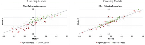
From Table 3, it can be seen that the correlations between the estimates from Models 0 and 7 for the one-step and two-step models are 0.903 and 0.947, respectively. Consistent with these correlations, the school effects from the one-step model are more sensitive to model specification than those from the two-step model, as illustrated by their larger spread around the trend line. Moreover, to illustrate the nature of the systematic differences across model specifications, two sets of schools are highlighted in the figure—schools with high free/reduced-price lunch shares and schools with low free/reduced-price lunch shares. High free/reduced-price lunch schools are defined as schools with 80% or more eligible students; low free/reduced-price lunch schools are schools with 20% or fewer eligible students.¹⁴ Looking at the first panel of Figure 1, which plots the results from the one-step model, the sensitivity of the estimates for these two groups of schools is in line with what one would expect—disadvantaged schools have systematically higher estimates if we use Model 0 (they are below the trend line), while advantaged schools have systematically lower estimates (above the trend line). For the two-step model a similar pattern emerges, but very weakly. The reason is that the lagged average test score for schools, which is included even in Model 7 within the two-step framework, serves as a good proxy for the other omitted student- and school-level control variables.¹⁵

Table 5. Correlations between VAM estimates and school-level averages for key student characteristics (Communication arts)

	Correlation with	Correlation with avg.	Top 25% avg.	Bottom 25% avg.	Top 25% avg.	Bottom 25% avg.
	avg. FRL	lagged score	free lunch	free lunch	lagged score	lagged score
One-step model
Model 0	−0.22**	0.27**	45.8	57.6	0.07	−0.12
Model 1	−0.30**	0.31**	43.2	59.3	0.09	−0.14
Model 2	−0.28**	0.34**	44.3	58.9	0.09	−0.16
Model 3	−0.34**	0.37**	43.5	59.9	0.09	−0.15
Model 4	−0.31**	0.38**	43.3	57.4	0.11	−0.13
Model 5	−0.41**	0.43**	39.7	59.5	0.14	−0.14
Model 6	−0.40**	0.50**	41.1	60.6	0.15	−0.18
Model 7	−0.50**	0.54**	38.2	61.7	0.17	−0.18
Two-step model
Model 0	0.05	−0.03	51.3	49.9	−0.03	0.00
Model 1	−0.04	−0.07	49.4	52.9	−0.06	0.00
Model 2	0.04	−0.02	50.8	49.6	−0.03	−0.02
Model 3	−0.04	−0.07	49.0	53.3	−0.06	−0.00
Model 4	0.05	−0.02	51.6	50.2	−0.03	−0.00
Model 5	−0.04	−0.06	48.3	54.0	−0.04	−0.02
Model 6	0.04	−0.01	51.0	49.5	−0.02	0.00
Model 7	−0.05	−0.05	49.3	53.4	−0.06	−0.00

**Correlation is significant at the 1% level. *Correlation is significant at the 5% level. NOTE: The by-quartile averages are calculated as simple averages across schools. There are strong negative correlations in the data between school size and free-lunch status and test scores (many small, rural schools in Missouri have high free-lunch shares and low scores), which explains why the simple averages for free/reduced-price lunch share presented here are large compared to what we report for the student-level sample in Table 1. Average test scores for the top and bottom quartiles are centered on the school-level sample average for ease of presentation.

Table 5A. Correlations between teacher-level VAM estimates and teacher-level averages for key student characteristics (Communication arts)

	Correlation with	Correlation with avg.	Top 25% avg.	Bottom 25% avg.	Top 25% avg.	Bottom 25% avg.
	avg. FRL	lagged score	free lunch	free lunch	lagged score	lagged score
One-step model
Model 0	−0.34**	0.34**	38.0	62.6	0.18	−0.24
Model 1	−0.39**	0.38**	34.8	64.1	0.21	−0.28
Model 2	−0.43**	0.41**	33.6	66.1	0.23	−0.30
Model 3	−0.48**	0.44**	29.3	67.7	0.28	−0.33
Model 4	−0.43**	0.45**	34.7	67.2	0.24	−0.32
Model 5	−0.48**	0.49**	31.5	68.3	0.28	−0.34
Model 6	−0.55**	0.53**	27.6	70.6	0.33	−0.37
Model 7	−0.61**	0.59**	24.9	71.0	0.36	−0.38
Two-step model
Model 0	−0.08	0.08	47.1	51.1	−0.01	−0.07
Model 1	−0.12*	0.08	44.4	52.5	0.02	−0.06
Model 2	−0.08	0.10	46.8	52.6	0.01	−0.10
Model 3	−0.22**	0.09	41.6	57.1	0.04	−0.10
Model 4	−0.05	0.06	47.9	52.8	−0.01	−0.08
Model 5	−0.12*	0.06	48.3	54.3	−0.03	−0.07
Model 6	−0.06	0.09	48.4	52.6	−0.01	−0.09
Model 7	−0.27**	0.10*	40.8	60.0	0.00	−0.15

**Correlation is significant at the 1% level. *Correlation is significant at the 5% level. NOTE: The by-quartile averages are calculated as simple averages across teachers. Average test scores for the top and bottom quartiles are centered on the teacher-level sample average.

Building on Figure 1, Tables 4 and 5 compare schools’ VAM estimates with two school-aggregated characteristics: (1) the percentage of students who are eligible for free/reduced-price lunch and (2) the average lagged test score (subject specific). Table 5 shows results for math, and Table 6 shows results for communication arts. The rows in each table correspond to the different models. As mentioned previously, all models are estimated using a constant estimation sample to ensure that the findings are not confounded by changes to the data. The first two columns report correlations between the VAM estimates and the school-aggregated characteristics. The remaining four columns report the average characteristics of schools in the top and bottom quartiles based on the VAM rankings from the different specifications.¹⁶ These groups can be thought of as hypothetical “winners” and “losers” from a simple evaluation system based solely on the VAM.¹⁷

In the one-step models, the first two columns of the tables show that there are nonnegligible correlations between the VAM estimates and school-level aggregates throughout. Unsurprisingly, the correlations are largest in the models that include the fewest student-level controls. Corresponding to these correlations, the highest and lowest value-added schools as identified by the one-step models are more-clearly differentiated in terms of their students. In all of the one-step specifications and in both subjects, top-quartile schools consistently have fewer low-income students and students with higher prior performance. Alternatively, the two-step models produce VAM estimates that are mostly uncorrelated with school-level aggregates. This is because the two-step models purposefully partial out the variance in student outcomes associated with the school-level aggregates prior to estimating the growth measures, whereas in the one-step models the school-level aggregates are absorbed by the school fixed effects.¹⁸

Table 6. Average free/reduced-lunch percentages in schools that finish in the top value-added quartile based on estimates from either the One-Step or Two-Step versions of Model 0, but not both

	N	F/RL%
One-step only—math	29	41.1
One-step only—communication arts	15	37.4
Two-step only—math	29	53.9
Two-step only—communication arts	15	69.2

NOTE: There are 348 schools included in our analysis (see Table 1).

Table 6 provides one additional set of results related to the disparities in output across the models. Specifically, we identify the nonoverlapping hypothetical “winners” from the one-step and two-step versions of Model 0—that is, the schools that are in the top quartile based on the output from one model but are not in the top quartile using the other model (this breakdown follows Ehlert et al. 2013). In the table we report differences between the groups in terms of the student share on free/reduced-price lunch. Consistent with Figure 1 and Tables 4 and 5, the two-step model replaces a group of relatively more-advantaged schools with a group of less-advantaged schools in the top quartile.

4.2 Teacher-Level Findings

We replicate our school-level analysis for teachers using data from our cluster of St. Louis area districts. Our findings are reported in Tables 3A–6A, which are analogous to Tables 3–6 above. In addition, Appendix Table A.1A provides the teacher-level analog to Appendix Table A.1.

Our teacher-level findings are similar to our school-level findings throughout. In fact, substantively, the teacher-level analysis reveals no new insights regarding the use of the various VAM specifications. Because of the strong similarity in our findings between the school- and teacher-level models, we refrain from a lengthy discussion of our teacher-specific analysis.¹⁹

Table 6A. Average free/reduced-lunch percentages for teachers that finish in the top value-added quartile based on estimates from either the one-step or two-step versions of Model 0, but not both

	N	F/RL%
One-step only—math	21	25.9
One-step only—communication arts	19	21.2
Two-step only—math	21	61.4
Two-step only—communication Arts	19	67.3

5. DISCUSSION AND CONCLUSION

We provide side-by-side comparisons of various VAMs that differ in terms of which controls are included in the models and how the controls are included. We highlight two key findings from our study. First, VAMs that include shorter test score histories perform fairly well compared to those with longer score histories and do not systematically favor particular types of schools or teachers. An implication of this finding is that policymakers should consider carefully the costs and benefits associated with complicating standard models along this dimension. A particularly important tradeoff associated with increasing test-score-history requirements within the standard VAM framework is that each additional year of required prior performance results in structurally missing data. For example, going from requiring a single lagged score to requiring two lagged scores necessitates that grade-4 students will have incomplete records (in the typical testing regime that starts in grade-3). Some approaches, like SGPs, simply use whatever score histories are available for each student. This may or may not be desirable—an important conceptual weakness of such an approach is that it implicitly uses different modeling structures to evaluate the performance of different educators.

The second key finding from our study is that the decision about whether to control for student covariates and schooling environments, and how to control for this information, influences which types of schools and teachers are identified as top and bottom performers. Models that are less aggressive in controlling for student characteristics and schooling environments systematically identify schools and teachers that serve more advantaged students as providing the most value-added, and correspondingly, schools and teachers that serve more disadvantaged students as providing the least. Given recent arguments in favor of using equally circumstanced comparisons in education evaluations (Barlevy and Neal 2012; Ehlert et al. 2013)—that is, comparisons between schools and teachers that serve similar student populations—this is an important consideration for state and local education agencies that are exploring the use of value-added models as a part of their accountability systems.

Notes

Recent “Race to the Top” legislation encourages states to design teacher evaluation systems based on student achievement. Some of the winning proposals attached consequences to VAM-based assessments including tenure denial and tenure revocation. Other federal programs, like the Teacher Incentive Fund, also encourage achievement-based teacher evaluations. In addition, locales from Washington, DC, to New York City to the state of Missouri are experimenting with VAM-based accountability in a variety of forms.

Although the research literature on growth modeling is vast, most studies do not illustrate the tradeoffs that come with choosing different VAM specifications (a recent exception is Goldhaber et al. 2012). The VAM literature is too large to cite individual studies but a useful starting point for the interested reader is McCaffrey et al. (2003); for a recent overview article see Hanushek and Rivkin (2010).

With approaches like standard Student Growth Percentiles (SGPs) (Betebenner 2009), which use whatever score history is available for each student, this is less of a concern. However, a tradeoff that comes from using different score histories for different students is that it effectively means that different schools and/or teachers are evaluated using different models. As a specific example, in a teacher-level analysis, grade-4 teachers would be evaluated using a single-lagged-score model but grade-6 teachers would mostly be evaluated using a model that includes information from three lagged scores.

In omitted results we confirm that there are not strong ceiling effects in the MAP exam following Koedel and Betts (2010).

Recent studies show that using multiple years of student outcome data to produce measures of value added offers several benefits (Goldhaber and Hansen, 2013; Koedel and Betts, 2011; McCaffrey et al. 2009). However, the qualitative insights from our sensitivity analysis based on single-year VAMs will carry over to multi-year VAMs.

For analyses conducted at the elementary school level, models that require more than one year of lagged test-score data result in structurally missing data—for example, models that require a second lagged score necessarily exclude grade-4 students (given a standard testing regime starting in grade-3, as in Missouri).

The district cluster includes the St. Louis Public School District, which has an enrollment of approximately 25,000 students. Most of the surrounding districts are much smaller (the average enrollment in the remaining 15 districts is 6,000 students).

If a student has the same teacher for more than one section in the relevant subject, the aggregate used for that student is the average of the relevant measures across all the sections.

Ehlert et al. (2013) provided an extended discussion of this feature of the two-step model, which they refer to as “proportionality.” In the present application the two-step model is more effective in achieving proportionality in our school-level models than in our teacher-level models. An important reason is that we use classroom-aggregated student characteristics in our teacher-level models, which are not the same as teacher-aggregated characteristics (across classrooms). This is reflected in the results presented below. As discussed by Ehlert et al. (2013), if proportionality were a targeted objective in our teacher level models, there are straightforward ways to achieve it.

Raudenbush and Willms (1995) provide a useful alternative discussion of similar issues.

From the perspective of parents, for example, this type of confounding information may be unimportant (in the sense that parents may only care about the total school effect, regardless of the source). However, this is not the case for school administrators or regulatory agencies attempting to evaluate the performance of education personnel, schools, and districts.

With one exception. The correlation for the Model-4 version of the two-step VAM in communication arts is higher than for Model 3.

As noted previously, the single-lagged-score VAMs in Table 3 are estimated using the same sample that we use to estimate Model 0 so that the effects of the specification adjustments are not confounded with the effects of adjustments to the estimation sample. However, larger data samples are available to estimate the single-lagged-score VAMs because students with missing second- and third-lagged scores can be included. Appendix Table A.1 uses the larger data samples to replicate the analysis in columns (5) through (7). Our findings using the larger samples are very similar to what we report in Table 3.

The patterns illustrated in Figure 1 are not sensitive to using reasonable, alternative definitions.

Another interesting aspect of Figure 1 is that, for the one-step model, most of the high-FRL school effect estimates are in the lower left-hand quadrant of the graph, that is, their effect estimates from both models (0 and 7) are below average, while the reverse is true for low-FRL schools. A similar pattern is not present (or appears only weakly) for the two-step model. We elaborate on this point below.

Sampling variation is surely contributing to which schools are identified in the top and bottom groups based on the simple comparisons as reported in Tables 5 and 6 (Kane and Staiger 2002). In an actual evaluation, incorporating information about the error variance associated with each school's value-added estimate can partly mitigate the role of sampling variability in terms of dictating winners and losers.

Here, the terms “winners” and “losers” are not meant to be relative to the “true” effect estimates, which are of course unknown. Rather, we simply aim to identify schools that will receive hypothetical commendations or sanctions from the evaluation system given the results of the different model specifications.

Note that even the correlations for the estimates from the two-step version of Model 7 are mostly small. The small correlations are driven by the inclusion of aggregate lagged test scores in the first step, which as we noted earlier functions as an effective proxy for schooling environments.

It should also be noted that our teacher-level models do not include controls for observable qualifications (e.g., teacher experience, education levels, etc.), as the teacher-level analysis was designed to parallel the school-level analysis for comparability purposes. If policymakers wish to compare similarly qualified teachers (perhaps most importantly along the dimension of experience), then explicit experience controls could be added to the general specification we use here. Notable recent studies that investigate differences in teacher performance by experience level include Clotfelter et al. (2006) and Wiswall (2011).

APPENDIX: Correlations From Single-Lagged-Score Models that Use All Available Data

Table A.1. Correlation Table for school-level VAM estimates from single-lagged-score models using all available data. All models are compared to Model 4 using a fixed estimation sample

	Model 5	Model 6	Model 7
One-step model
Math	0.992	0.985	0.973
Communication arts	0.989	0.964	0.943
Two-step model
Math	0.991	0.997	0.974
Communication arts	0.981	0.987	0.954

Table A.1A. Correlation Table for teacher-level VAM estimates from single-lagged-score models using all available data. All models are compared to Model 4 using a fixed estimation sample

	Model 5	Model 6	Model 7
One-step model
Math	0.997	0.991	0.979
Communication arts	0.997	0.977	0.959
Two-step model
Math	0.995	0.996	0.974
Communication arts	0.981	0.986	0.909

REFERENCES

- Aaronson, D., Barrow, L., and Sander, W. (2007), “Teachers and Student Achievement in the Chicago Public High Schools,” Journal of Labor Economics, 25, 95–135.
- Barlevy, G., and Neal, D. (2012), “Pay for Percentile,” American Economic Review, 102, 1805–1831.
- Betebenner, D.W. (2009), “Norm- and Criterion-Referenced Student Growth,” Educational Measurement: Issues and Practice, 28, 42–51.
- Betts, J. (1995), “Does School Quality Matter? Evidence From the National Longitudinal Survey of Youth,” Review of Economics and Statistics, 77, 231–250.
- Clotfelter, C.T., Ladd, H.F., and Vidgor, J.L. (2006), “Teacher-Student Matching and the Assessment of Teacher Effectiveness,” Journal of Human Resources 41, 778–820.
- Ehlert, M., Koedel, C., Parsons, E., and Podgursky, M. (2013), “Selecting Growth Measures for School and Teacher Evaluations: Should Proportionality Matter?” CALDER Working Paper No. 80.
- Goldhaber, D., Walch, J., and Gabele, B. (2012), “Does the Model Matter? Exploring the Relationship Between Different Student Achievement-Based Teacher Assessments,” . CEDR Working Paper 2012–2016.
- Goldhaber, D., and Hansen, M. (2013). “Is It Just a Bad Class?: Assessing the Long-Term Stability of Estimated Teacher Performance,” Economica, 80, 589–612.
- Han, B., McCaffrey, D.F., Springer, M., and Gottfried, M. (2012), “Teacher Effect Estimates and Decision Rules for Establishing Student-Teacher Linkages: What are the Implications for High-Stakes Personnel Policies in an Urban School District?” Statistics, Politics, and Policy, 3, 2051.
- Hanushek, E. (1996), “Measuring Investment in Education,” Journal of Economic Perspectives, 10, 9–30.
- Hanushek, E.A., and Rivkin, S.G. (2010), “Generalizations About Using Value-Added Measures of Teacher Quality,” American Economic Review (P&P), 100, 267–271.
- Kane, T.J., and Staiger, D.O. (2002), “The Promises and Pitfalls of Using Imprecise School Accountability Measures,” Journal of Economic Perspectives, 16, 91–114.
- Koedel, C., and Betts, J.R. (2010), “Value-Added to What? How a Ceiling in the Testing Instrument Affects Value-Added Estimation,” Education Finance and Policy, 5, 54–81.
- ——— (2011), “Does Student Sorting Invalidate Value-Added Models of Teacher Effectiveness? An Extended Analysis of the Rothstein Critique,” Education Finance and Policy, 6, 18–42.
- McCaffrey, D.F., Lockwood, J.R., Koretz, D.M., and Hamilton, L.S. (2003), Evaluating Value-Added Models for Teacher Accountability, Santa Monica, CA: The RAND Corporation.
- McCaffrey, D.F., Lockwood, J.R., Sass, T.R., and Mihaly, K. (2009), “The Inter-Temporal Variability of Teacher Effect Estimates,” Education Finance and Policy, 4, 572–606.
- Raudenbush, S., and Willms, D.J. (1995), “The Estimation of School Effects,” Journal of Educational and Behavioral Statistics, 20, 307–335.
- Sass, T.R., Hannaway, J., Xu, Z., Figlio, D.N., and Feng, L. (2012), “Value Added of Teachers in High-Poverty Schools and Lower Poverty Schools,” Journal of Urban Economics, 72, 104–122.
- Wiswall, M. (2013), “The Dynamics of Teacher Quality,” Journal of Public Economics, 100, 61–78.