Signal Weighted Teacher Value-Added Models

Abstract

This study introduces the signal weighted teacher value-added model (SW VAM), a value-added model that weights student-level observations based on each student’s capacity to signal their assigned teacher’s quality. Specifically, the model leverages the repeated appearance of a given student to estimate student reliability and sensitivity parameters, whereas traditional VAMs represent a special case where all students exhibit identical parameters. Simulation study results indicate that SW VAMs outperform traditional VAMs at recovering true teacher quality when the assumption of student parameter invariance is met but have mixed performance under alternative assumptions of the true data generating process depending on data availability and the choice of priors. Evidence using an empirical dataset suggests that SW VAM and traditional VAM results may disagree meaningfully in practice. These findings suggest that SW VAMs have promising potential to recover true teacher value-added in practical applications and, as a version of value-added models that attends to student differences, can be used to test the validity of traditional VAM assumptions in empirical contexts.

Keywords:

• Simulation study
• Student characteristics
• Teacher accountability
• Teacher value-added

1 Introduction

Teacher value-added models (VAMs) are a method for estimating a teacher’s effectiveness based on their students’ outcomes, and research has repeatedly demonstrated that VAMs represent real impacts of teacher quality. Kane and Staiger (2008) estimated that a one standard deviation increase in teacher value-added causes between 0.1 and 0.2 standard deviations increases in student test scores. Chetty et al. (2011) contextualized this estimate for Kindergarten teachers: a one standard deviation difference in VAMs translates to present-value earning gains of about $5350–$10,700 per student. Other research has found positive effects between teacher VAM estimates and student college matriculation rates, future earnings, and lower incidences of teenage pregnancy (Chetty, Friedman, and Rockoff 2014).

Such promising reports between VAM estimates and student outcomes have encouraged states to implement VAMs into their teacher evaluation systems specifically, during the Race to the Top era of the U.S. educational policy (Rotherham and Mitchel 2014), and such systems commonly informed decisions regarding performance bonuses, targeted professional development, and even dismissals and tenure (Harris and Herrington 2015). Since the passage of the Every Student Succeeds Act in 2015, VAMs are less commonly used for consequential decisions, but many school districts still employ VAMs and some states still actively encourage the use of VAMs, even if only for informational or formative purposes (Close, Amrein-Beardsley, and Collins 2019).

Despite their diminished popularity in education policy, VAMs as a research topic are still very relevant. Researchers are still developing novels ways to measure teacher impacts on students via VAMs, for example with noncognitive skills (Jackson 2018). And the demonstrated ability of VAMs to capture teacher effects has inspired similar techniques in a variety of contexts: Mulhern (2020) uses the same models to evaluate guidance counselor value-added, and Bacher-Hicks and de la Campa (2020) estimate New York City police commanders’ effects on stop and frisk tactics. But value-added models must be carefully employed, their analytic potential notwithstanding. After the proliferation of VAMs in teacher evaluation systems, multiple groups have successfully argued in court that VAM usage has caused harm, as such models were too inaccurate, flawed, and arbitrary to inform high stakes decisions (Amrein-Beardsley and Close 2019).

The validity of teacher VAMs is directly tied to their ability to measure true underlying teacher quality. If teacher quality were constant across time, model covariates perfectly accounted for year-to-year variability, and VAMs measured teacher quality without error, then the correlation between teacher VAM estimates from any two years would be a perfect 1. This is not the case. The highest correlation that Koedel, Mihaly, and Rockoff (2015) found among their review of studies was 0.64, and the lowest was 0.18. Some researchers have posited that such low stability across years may invalidate the use of VAMs for certain high stakes decisions (Amrein-Beardsley and Collins 2012). Teacher tenure decisions, for example, are often based on just a few years of observed performance, and thus VAMs could only measure that performance with questionable reliability (Sass 2008). A truly fantastic teacher could possibly be denied tenure due to a string of bad luck. Part of this inconsistency across years may be due to real changes in teacher quality (e.g., new teachers often improve substantially early in their career (Papay and Kraft 2015)), and another part may be due to random forces outside the purview of a teacher’s responsibility and thus VAMs (e.g., one classroom’s students were particularly affected by COVID related absences). However, some of this instability may be the fault of VAMs improperly modeling the variance structure of the student-level data provided.

The typical value-added model regresses student outcomes on multiple covariates, including a set of teacher assignment indicator variables which summarize the average association between being assigned to a given teacher and the outcome variable (Koedel, Mihaly, and Rockoff 2015). Past studies have proposed alternative model specifications which could further reduce estimation error (for some examples see: Rothstein 2009; Karl, Yang, and Lohr 2013; Ehlert et al. 2013; Lockwood and McCaffrey 2014) , but most proposed models operate with the assumption that every student’s performance is equally and comparably informative of teacher quality.

Two notable advances in VAMs literature have suggested models to the contrary. The first considers the possibility that students can be differentially responsive to the same teacher, so each student–teacher pair results in an “effective” teacher quality (i.e., student dependent quantity), distinct from underlying teacher quality (i.e., student independent quantity) (Jackson 2018; Mulhern 2020). Though this distinction is important, the cited studies essentially concede that VAMs only capture effective teacher quality, even though underlying teacher quality is more relevant when attempting to compare teachers. The second advance posits that value-added estimate precision may be a function of classroom composition and student characteristics. Herrmann, Walsh, and Isenberg (2016) find that modeling heteroscedasticity in empirical Bayes shrinkage procedures reveals students who have lower prior achievement and who receive free lunch tend to produce less precise value-added estimates. This result was corroborated by Stacy, Guarino, and Wooldridge (2018) who examined the association between the size of model residuals and student characteristics to conclude teachers assigned more lower performing students had less precise and less stable estimates across time. These investigations offer convincing evidence that precision varies across student characteristic groups but fall short of offering a solution to correct for this fact when calculating teacher value-added.

The present article builds on this line of inquiry by introducing the signal-weighted value-added model (SW VAM), whose functional form allows each student to demonstrate different levels of reliability (i.e., how noisy a student’s outcomes are across time) and sensitivity (i.e., how responsive a student’s outcome is to their teacher’s quality). The SW VAM leverages the repeated observation of students to estimate individual student parameters and thereby measure teacher quality independent of student characteristics or classroom composition. A major contribution of the SW VAM is its ability to empirically capture individual student parameters rather than coarsen students into groups (Herrmann, Walsh, and Isenberg 2016) or arbitrarily derive parameters based on observables (Reckase and Martineau 2015). The SW VAM locates such variability entirely within time-stable student-level parameters which implicitly capture both observed characteristics (e.g., race/ethnicity, gender, prior achievement) and typically unobserved characteristics (e.g., motivation, parental involvement, persistent health issues).

In this article I introduce and investigate the SW value-added model as an alternative to traditionally specified value-added models. To accomplish this, I simulate a series of datasets according to different data generating processes, and for each dataset assess and compare the performance of each’s ability to capture true teacher quality. I then use an empirical dataset to demonstrate the viability of signal-weighted models for practical applications.

The article is organized as follows. In Section 2, I provide a general overview of traditional value-added models and describe the traditional model used in the simulation studies. In Section 3, I introduce the signal-weighted value-added model and its theoretical advantages and vulnerabilities. Section 4 outlines the parameters of the simulation studies and each of the scenarios. Section 5 presents the results of the simulation studies. Section 6 introduces an empirical dataset, and Section 7 presents the results of the empirical data analysis. Section 8 concludes with a discussion of the limitations of the study and suggestions for future research.

2 Overview of Traditional Value-Added Models

This section provides an overview of traditional value-added models. A common specification of the traditional value-added models takes the following form:(1) $$Y_{\mathit{ijt}}={\beta }_0+Y_{\mathit{ijt}-1}{\beta }_1+X_{\mathit{ijt}}{\beta }_2+{\gamma }_{\mathit{ijt}}$$(1) (2) $${\gamma }_{\mathit{ijt}}=\sum _{j=1}^N{I}_{\mathit{ijt}}{\theta }_j+{\mathrm{ϵ}}_{\mathit{ijt}}$$(2) where $Y_{\mathit{ijt}}$ is a test score for student iin classroom j in year t, $X_{\mathit{ijt}}$ is a vector of observable student characteristics, $I_{\mathit{ijt}}$ is an indicator variable that equals 1 if student i was assigned to classroom j in year t, ${\gamma }_{\mathit{ijt}}$ is the idiosyncratic error term before accounting for teacher assignment, and ϵ_ijt is the error term after accounting for teacher assignment. The coefficient θj represents the value-added for teacher j, which is expressed as a predictor of student performance after controlling for other model covariates. Other common specifications include school-level covariates, multiple lagged scores, and hierarchical modeling (McCaffrey et al. 2004; Guarino, Reckase, and Wooldridge 2015; Koedel, Mihaly, and Rockoff 2015). Across all variations, though, θj represents the treatment effect associated with assignment to teacher j, and the outcome of each student assigned to teacher jgives a signal of this treatment effect.

Note that the model described by Equations (2)(2) $${\gamma }_{\mathit{ijt}}=\sum _{j=1}^N{I}_{\mathit{ijt}}{\theta }_j+{\mathrm{ϵ}}_{\mathit{ijt}}$$(2) and (3)(3) $${\gamma }_{\mathit{ijt}}\sim N\left({\theta }_j,\sigma \right)$$(3) is referred to as the “two-step” model, which is less common than the alternative, “one-step” model. I present the traditional value-added model process via this two-step process to better highlight its theoretical overlap with the SW VAM. In the following simulations, which include no covariates aside from teacher assignment, the one-step and two-step model are mathematically equivalent (Ehlert et al. 2013). A one-step version of signal-weighted VAMs is also easily implementable.

Though various alternatives to ordinary least squares specification exist, by convention, one can represent the second-step residual in Equation (2)(2) $${\gamma }_{\mathit{ijt}}=\sum _{j=1}^N{I}_{\mathit{ijt}}{\theta }_j+{\mathrm{ϵ}}_{\mathit{ijt}}$$(2) as a series of normal distributions for each student i assigned to teacher j at time t:(3) $${\gamma }_{\mathit{ijt}}\sim N\left({\theta }_j,\sigma \right)$$(3) where the model estimates the teacher coefficients θ_j based on maximum likelihood. Notably, in the value-added context, the distribution for γ_ijt depends on teacher identity j, but is agnostic towards student identity i, a fundamental difference with the SW VAM.

To compare the performance of SW VAMs to traditional VAMs, this study will use a random effects model to represent traditional VAMs, as opposed to a fixed effects model which is more common in practice (Koedel, Mihaly, and Rockoff 2015). The simulated data will draw teacher effects from a normal distribution, and the SW VAM, as will be explained in the next section, will impose a normal prior on teacher effects. To highlight the unique contributions of the SW VAM (i.e., the modeling of student parameters), I employ a traditional VAM which also imposes a normal prior on teacher effects, (i.e., the random effects model).

3 Overview of Signal-Weighted Value-Added Models

The central idea of the signal-weighted value-added model is to leverage the repeated observation of a given student to estimate the parameters of an outcome distribution specific to that student. These additional parameters effectively weight each student’s outcomes in the value-added model by their strength and clarity as signals of their assigned teacher’s quality. The SW VAM can produce first-step residuals in a process identical to the first step of the two-step traditional value-added model. However, rather than employ Equation (3)(3) $${\gamma }_{\mathit{ijt}}\sim N\left({\theta }_j,\sigma \right)$$(3) in the second step, it models the second-step residuals for student i assigned to teacher j as(4) $${\gamma }_{\mathit{ijt}}\sim N\left({\alpha }_i{\theta }_j,\frac{1}{a_i}\right)$$(4)

In contrast to Equation (3)(3) $${\gamma }_{\mathit{ijt}}\sim N\left({\theta }_j,\sigma \right)$$(3) which assumed an outcome distribution dependent only on teacher quality, Equation (4)(4) $${\gamma }_{\mathit{ijt}}\sim N\left({\alpha }_i{\theta }_j,\frac{1}{a_i}\right)$$(4) models the distribution of the outcome γ_ijt as a function of teacher quality θ_j as well as a student specific reliability parameter, $a_{\mathrm{i}}$, and sensitivity parameter, α_i. The model in Equation (4)(4) $${\gamma }_{\mathit{ijt}}\sim N\left({\alpha }_i{\theta }_j,\frac{1}{a_i}\right)$$(4) could be described as an interacted random effects model with heterogeneous variance. Alternatively, however, SW VAMs could also be described as an Item Response Theory (IRT) model. Specifically, the closest analogue is the continuous response model proposed by Samejima (1973) and further developed by Wang and Zeng (1998). In the context of IRT, reliability and sensitivity are referred to as “discrimination” and “scaling” parameters, respectively. Notably absent is the difficulty parameter, b, which in the value-added context would be equivalent to student fixed effects. For parsimony, I do not employ student fixed effects in the data generating process or the estimation models. For a discussion on the link between student fixed effects and the difficult parameter, see Reckase and Martineau (2015).

From an IRT perspective, the signal-weighted value-added model assesses the underlying ability θ_j of examinee j based on an exam composed of items, each presenting its own measure of reliability and sensitivity, with responses expressed on a continuous scale. In this way, teacher value-added estimation can be considered theoretically analogous to an assessment of teacher ability (i.e., teacher quality), with an exam composed of a classroom of students. Then, for a teacher j with ability θ_j encountering student i with reliability parameter a_i, and sensitivity parameter α_i, SW VAMs model the student response according to Equation (4)(4) $${\gamma }_{\mathit{ijt}}\sim N\left({\alpha }_i{\theta }_j,\frac{1}{a_i}\right)$$(4) .

The two student-specific parameters, a and α, allow for flexible modeling of a student’s distribution of possible outcomes. The reliability parameter, a, characterizes the variability of a student’s performance across repeated observations, which includes any measurement error associated with the outcome; relatively high reliability students innately express lower variability, and are therefore more reliable signals of teacher quality. For example, a student with an intermittent chronic illness could have innately erratic exam performance as some flair ups coincide with some exam days. The sensitivity parameter, α, characterizes the sensitivity of a student’s outcome to teacher quality; high sensitivity students are more affected by differences in teacher quality. An example of a low sensitivity student is one who engages in extensive private tutoring after school, as their performance relies relatively less on their in-school teachers. However, low sensitivity should not be mistaken for low information. Low sensitivity and high reliability characterize a student for whom differences in teacher quality manifest as small magnitude effects to performance, but those small differences reliably signal teacher quality.

The signal-weighted value-added model relies on an assumption I refer to as the student parameter invariance assumption: every student’s parameters are identically expressed across teacher assignment and time (e.g., grades). Said another way, a student will be equally reliable and sensitive to teacher ability every school year and irrespective of their teacher. Though this unlikely to be true in reality, traditional value-added models assume the strictly less likely scenario wherein the a and α parameter are identical across teacher assignment, time, and students. That is, traditional VAMs further constrain all students to have identical reliability and identical sensitivity. I refer to this as the student parameter identity assumption.

These two assumptions bring up a critical question in value-added modeling: how can one compare teacher estimates, if each teacher’s estimates are derived from different sets of students? In a typical school, for example, two fourth grade teachers have no overlap in their classroom’s students. This presents no issue for the traditional value-added model, as all students possess identical parameters by assumption and are therefore interchangeable. The SW VAM in contrast uses the strictly weaker assumption of student parameter invariance. Two teachers may not have the same set of students, but the two classes of students may mix in the following years. If the model can recover student parameters using this repeated data, it can produce student-independent estimates of teacher quality. These student-independent estimates allow for direct teacher comparisons without relying on the student parameter identity assumption or the belief that teachers will have comparable students on average over many time points.

The signal-weighted value-added model, with its student parameters, allows for more discretionary interpretations of teacher quality signals than could traditional value-added models. This can be especially important when comparing across schools or districts. Consider a school where performance is highly variable from day to day, such as one whose exam conditions are highly affected by weather (e.g., leaking ceiling, underpowered HVAC, poor sound insulation). Students at this school would be relatively poor signals of their assigned teachers’ abilities, as underperformance on a given end-of-year exam could be the result of either low teacher quality, or unfortunately timed weather events. Whereas traditional VAMs would weight these students’ observations equal to the rest of the data, SW VAMs could down-weight these observations by estimating a low reliability parameter for such students.

Intrinsic to the accurate estimation of teacher quality using the signal-weighted value-added model is the accurate estimation of student parameters. The teacher value-added context typically uses datasets where teachers have dozens of relevant observations (in the form of every student assigned to the teacher), but each student is only observed a few times at most. This presents a challenge for signal-weighted value-added models. Because the model includes two parameters for each student, and one parameter for each teacher, the system would be statistically underidentified with only two or fewer observations for each student. Further, even with marginal overidentification the model may still demonstrate such considerable imprecision as to offset any potential gains in accuracy.

Imposing prior distributions on the student parameters can help guard the estimation process against such instability. A prior with thin tails, for example, would discourage the model from ascribing extreme parameter values and shrink estimates to the distribution center. Future research that employs the SW VAM in a context with sufficient data to accurately estimate student parameters (e.g., multiple assessments per student per academic year) may eventually derive the exact distribution shapes, but until such time I suggest researchers employing the SW VAM test the sensitivity of their results to their choice of priors. In the present study, I check the robustness of SW VAM performance to the choice of prior by repeating the estimation process using three different distributions, only one of which aligns with the true data generating process (log normal). The Weibull distribution and skewed normal distribution were chosen arbitrarily among the unimodal, continuous distributions available in the employed statistical software (unimodality and continuous being plausible properties of such distributions in reality). Note that a skew normal prior allows for negative values (which is unlikely true) and, as shown in the results, performed the worst among the signal-weighted models. I derive the signal-weighted model estimates using a Markov chain Monte Carlo (MCMC) method, which is more adaptable to contexts with complex priors than typical maximum likelihood estimation methods.

In the following simulations I investigate the theoretical strengths and limitations of the signal-weighted value-added model relative to the traditional value-added model. The potential advantage of SW VAMs is its use of the student invariance assumption, which involves estimation of underlying characteristics unique to each student but invariant across time and teacher assignment. Thus, the ideal scenario for SW VAMs to outperform traditional VAMs has four specific qualities. First, the dataset has enough observations per student to allow for meaningfully accurate estimation of student parameters. Second, the student parameter invariance assumption is true. But, third, the student parameters identity assumption is false. And fourth, the shapes of parameter priors are accurate. The following simulation scenarios assess the performance of SW VAMs and the importance of each of these four features to its performance.

All SW VAM estimations were conducted using the “stan” package in R (Stan Development Team 2018). Due to computational resource limitations, every signal-weighted model fit on the simulation data was conducted using one chain, which suggests the presented results may underestimate the true performance of signal-weighted models. For the empirical data example in the later sections, I use four chains for each signal-weighted model fit.

4 Simulated Data

The simulation study investigates the relative performance of SW VAMs across three theoretical data generating scenarios. I quantify the relative ability of each method using two primary metrics. First, I consider correlation between estimated teacher quality and true teacher quality, where higher correlation suggests better performance. Note that correlations are unit invariant, which aligns with practical uses of teacher VAM estimates as measures of relative quality. The second metric we calculate is the proportion of teachers whose performance category is correctly identified, where each category is defined by dividing the range of teacher quality estimates into equal fourths. This roughly mirrors the IMPACT teacher-evaluation system implemented in District of Columbia Public Schools, which also used four discrete performance categories (Dee and Wyckoff 2015).

Each dataset is composed of a set of 20 teachers per grade (teachers only teach one grade) and 400 students (evenly distributed as 20 students per classroom). Teacher parameters are drawn from a standard normal distribution, and student reliability and sensitivity parameters are drawn from log normal distributions.(5) $$\begin{array}{c}{\theta }_j\sim N\left(0,1\right)\\ a_i\sim \mathit{logN}\left(\log \left(1\right),\frac{\log \left(2\right)}{2}\right)\\ {\alpha }_i\sim \mathit{logN}\left(\log \left(0.2\right),\frac{\log \left(2\right)}{2}\right)\end{array}$$(5)

For the purposes of the present study, I arbitrarily choose log normal distributions based on the theoretical limits of the student parameters (e.g., reliability parameter must be greater than 0) and ease of interpretation. The distribution parameters in Equation (5)(5) $$\begin{array}{c}{\theta }_j\sim N\left(0,1\right)\\ a_i\sim \mathit{logN}\left(\log \left(1\right),\frac{\log \left(2\right)}{2}\right)\\ {\alpha }_i\sim \mathit{logN}\left(\log \left(0.2\right),\frac{\log \left(2\right)}{2}\right)\end{array}$$(5) were based on the results of Kane and Staiger (2008), which used standardized test scores as the outcome. Specifically, I start by setting the teacher parameter distribution as a standard normal distribution. Kane and Staiger report that a standard deviation difference in teacher effects demonstrates about a 0.2 standard deviation impact on the outcome across subjects and model specifications, so I set the center of the sensitivity parameter distribution at 0.2. Thus, in terms of our data generating process, raising teacher quality by one standard deviation adds 0.2 to an average student’s expected outcome. In rough terms, a standard normal multiplied by 0.2 has an effective variance of 0.04, leaving 96% of the outcome variance unaccounted for. This would suggest a reliability (i.e., residual noise) parameter of 0.98, the square root. However, rather than set the center of the reliability parameter distribution at 0.98, I round up to 1 for simplicity, recognizing that as a result the outcome will no longer have a total variance of 1 in our simulations. As no empirical data on the true distribution of these student parameters exists, I arbitrarily impose that 95% of the log normal distributions exist between half and twice the center values. Students were assigned randomly to one teacher per grade, with every student appearing in the data exactly once per grade. For each observed teacher–student pair, the data generating process randomly drew an outcome according to the relevant teacher and student parameters and the model given in Equation (4)(4) $${\gamma }_{\mathit{ijt}}\sim N\left({\alpha }_i{\theta }_j,\frac{1}{a_i}\right)$$(4) . Note that in these simulations I directly generate the second-stage residuals as the outcome variable, which in practice presumes sufficient data to calculate second-stage residuals, such as student characteristics and baseline test scores.

For each generated dataset, I estimate one set of teacher quality estimates according to the traditional value-added model as described in Equation (3)(3) $${\gamma }_{\mathit{ijt}}\sim N\left({\theta }_j,\sigma \right)$$(3) , and three sets according to the signal-weighted value-added model as described in Equation (4)(4) $${\gamma }_{\mathit{ijt}}\sim N\left({\alpha }_i{\theta }_j,\frac{1}{a_i}\right)$$(4) . The three SW VAM estimates differ in the prior imposed on student characteristics for the estimation process. One aligns with the true data generating process (log normal), and two intentionally do not (Weibull and skew normal). The Weibull and skew normal distributions are unimodal, but whereas the log normal and Weibull distributions observe a theoretical lower bound of 0, the skew normal does not.

I consider three sets of scenarios (A, B, and C), where each set contains three parallel data generating processes with two grades, three grades, and four grades of observations per student, and each scenario comprises of 100 independently generated trials. The various scenario characteristics are summarily displayed in Table 1. Notably, in some trials the traditional VAM returned the same value for all teacher quality estimates, the random effects model estimating that all teacher effects were identical. In the main results presented below, I excluded these cases, as they presented as outliers on the performance measures. Additional simulations were conducted until 100 valid simulations were achieved for every scenario.

Table 1 Characteristics of each of the data generating scenarios and the number of trials in which the traditional value-added model estimated zero variance across teacher estimates.

Scenario	Student Parameter	Number	Additional
	Generating	of Grades	Trials
	Assumption		Needed
A-2	Invariance	2	1
A-3	Invariance	3	0
A-4	Invariance	4	0
B-2	Identity	2	9
B-3	Identity	3	4
B-4	Identity	4	8
C-2	Random	2	1
C-3	Random	3	0
C-4	Random	4	1

In the A-scenarios, the student parameters were generated “invariantly”: every student had their own set of parameters and retained these parameters for every generated outcome. This scenario aligns with the signal-weighted value-added model assumption of student parameter invariance and describes the case where student parameters are invariant across time. SW VAMs should outperform traditional VAMs in the A-scenarios if the MCMC estimation procedure, guided by the imposed priors, can successfully accommodate the large number of parameters. Otherwise, the traditional model’s oversimplification of the data structure may be a worthwhile tradeoff. As the number of observations per student increases, the SW VAM estimates should become more stable, improving the relative performance of the signal-weighted model.

In the B-scenarios, student parameters were generated “identically”: one set of parameters was drawn from the student parameter distributions described in Equation (6) and assigned to every student for every generated outcome. This scenario aligns with the traditional value-added model assumption of student parameter identity, that is, all students are interchangeable with respect to signaling teacher quality. Traditional VAMs should outperform signal-weighted VAMs in the B-scenarios, as the signal-weighted model unnecessarily attends to perceived student parameter differences, introducing extraneous model variance. I expect SW VAMs to improve marginally with additional years, as this should improve student parameter estimation (toward the same value). However, SW VAMs will always be at a strict disadvantage. Whereas SW VAMs will use two, three, or four observations to estimate each student’s parameters (which are in fact identical), traditional VAMs will leverage every student observation to estimate the one relevant a- and α-parameter.

In the C-scenarios student parameters were generated “randomly”: every student received an independently drawn set of parameters for every generated outcome. This scenario describes the situation where student parameters vary between students and are uncorrelated over time within students. It is not obvious which model will perform better in the C-scenarios, as both models’ assumptions are incorrect. The traditional value-added model will estimate a middling reliability and sensitivity parameter across all students. The signal-weighted model should also tend to estimate middling parameters for each student, as on average student parameters are uncorrelated across grades. However, by chance some students will be assigned similar parameters across grades of observation. If SW VAMs can identify these students (e.g., down weighting students with large outcome swings as low reliability), while also conservatively assigning middling parameters to students who presented middling parameters on average, SW VAMs should outperform traditional VAMs. On the other hand, if SW VAMs cannot correctly distinguish between these cases, then attending to student parameters will cause greater instability. Additional grades of observation may improve the performance of SW VAMs in some regards. For example, fewer students will possess similar parameters across all grades by chance, but the model will more consistently identify such students when they do occur. With fewer exceptional students to leverage, the signal-weighted model could operate more similarly to the traditional model, so the margin of outperformance may diminish even if the margin of outperformance become more stable overall.

Admittedly, none of the A, B, or C scenarios are likely to be true in practice. Students likely have distinct parameters, but these are probably liable to some change over time (e.g., a student incurs a chronic illness, or enrolls in private tutoring, for only some grades of observation). However, by comparing model performance under these three extremes, the simulations illustrate best- and worst-case scenarios, boundaries on expected relative performance in real world settings. Notably, as shown in the next section, simulation results suggest that likelihood aside even under the worst-case scenario for SW VAMs, the SW VAM can still perform relatively well, which should encourage practitioners to employ the method on their own data.

5 Simulation Results

The results presented in Tables 2 and 3 largely confirm the previously stated hypotheses. With respect to either of the primary metrics of performance (Figures 1 and 2), when the data generating process aligned with the signal-weighted model assumptions, as in the A-scenarios, the signal-weighted model using the log normal prior consistently outperformed the traditional model, less consistently with the Weibull prior, and still less with the skew normal prior. The reverse was true for the B-scenarios, where all the signal-weighted models performed poorly compared to the traditional model on correlation with true values but had mixed performance when recovering teacher quartiles. When the data generating process aligned with neither model (C-scenarios), the SW VAM outperformed the traditional VAM for only some of the prior specifications, the skew normal scenario falling noticeably short.

Fig. 1 Difference in the proportion of teachers whose quality quartile is correctly identified between the SW model and the traditional model.

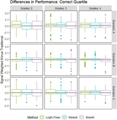
Fig. 2 Difference in the correlation of estimated teacher quality to true teacher quality between the SW model and the traditional model.

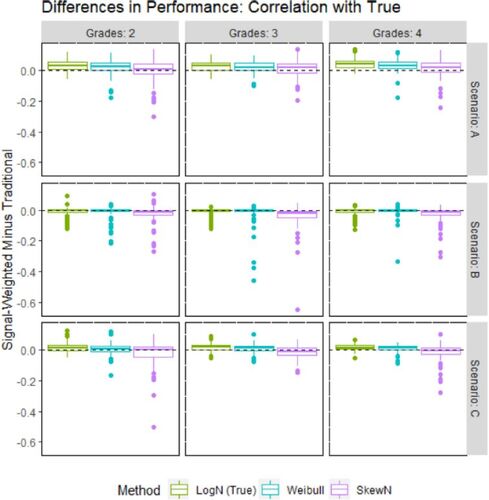
Table 2 Performance and relative performance across models with regard to correctly identifying teachers’ quality quartile.

	Proportion correctly identified quartile
	Traditional	Log Normal prior	Weibull prior	Skew normal prior
	mean	minus traditional	minus traditional	minus traditional
A-2	0.447	0.024${}^{\ast \ast \ast }$	0.006	0.007
	(0.089)	(0.007)	(0.007)	(0.008)
A-3	0.472	0.015${}^{\ast }$	0.014${}^{\ast }$	0.007
	(0.076)	(0.007)	(0.006)	(0.006)
A-4	0.477	0.015${}^{\ast \ast }$	0.011${}^{\ast }$	0.006
	(0.071)	(0.005)	(0.005)	(0.006)
B-2	0.499	–0.011${}^{\ast }$	–0.008	–0.013${}^{\ast }$
	(0.129)	(0.004)	(0.006)	(0.006)
B-3	0.500	–0.002	–0.001	–0.012${}^{\ast }$
	(0.111)	(0.003)	(0.004)	(0.006)
B-4	0.510	–0.004	–0.001	–0.016${}^{\ast \ast \ast }$
	(0.114)	(0.004)	(0.004)	(0.005)
C-2	0.457	0.006	–0.000	–0.009
	(0.080)	(0.007)	(0.006)	(0.007)
C-3	0.468	0.009	0.007	–0.004
	(0.075)	(0.006)	(0.006)	(0.007)
C-4	0.468	0.011${}^{\ast }$	0.008	–0.002
	(0.068)	(0.005)	(0.005)	(0.006)

Standard deviations displayed in parentheses; statistical significance calculated using paired t-test ${}^{\ast }p<0.05$; ${}^{\ast \ast }p<0.01$; ${}^{\ast \ast \ast }p<0.001$.

Table 3 Performance and relative performance across models with regard to correlation between estimated teacher quality and true teacher quality.

	Correlation with true teacher quality
	Traditional	Log Normal prior	Weibull prior	Skew normal prior
	mean	minus traditional	minus traditional	minus traditional
A-2	0.629	0.029${}^{\ast \ast \ast }$	0.017${}^{\ast \ast \ast }$	0.003
	(0.094)	(0.004)	(0.005)	(0.007)
A-3	0.651	0.029${}^{\ast \ast \ast }$	0.021${}^{\ast \ast \ast }$	0.010${}^{\ast }$
	(0.080)	(0.003)	(0.004)	(0.005)
A-4	0.638	0.040${}^{\ast \ast \ast }$	0.033${}^{\ast \ast \ast }$	0.011${}^{\ast }$
	(0.071)	(0.003)	(0.004)	(0.005)
B-2	0.673	–0.012${}^{\ast \ast \ast }$	–0.015${}^{\ast \ast \ast }$	–0.022${}^{\ast \ast \ast }$
	(0.181)	(.003)	(0.004)	(0.005)
B-3	0.678	–0.010${}^{\ast \ast \ast }$	–0.020${}^{\ast \ast \ast }$	–0.040${}^{\ast \ast \ast }$
	(0.154)	(0.002)	(0.007)	(0.008)
B-4	0.665	–0.011${}^{\ast \ast \ast }$	–0.009${}^{\ast }$	–0.030${}^{\ast \ast \ast }$
	(0.176)	(0.003)	(0.004)	(0.005)
C-2	0.647	0.015${}^{\ast \ast \ast }$	0.005	–0.022${}^{\ast \ast }$
	(0.102)	(0.003)	(0.003)	(0.007)
C-3	0.632	0.017${}^{\ast \ast \ast }$	0.011${}^{\ast \ast \ast }$	–0.015${}^{\ast \ast }$
	(0.081)	(0.003)	(0.003)	(0.004)
C-4	0.628	0.016${}^{\ast \ast \ast }$	0.008${}^{\ast \ast \ast }$	–0.017${}^{\ast \ast }$
	(0.070)	(0.002)	(0.002)	(0.005)

Standard deviations displayed in parentheses; statistical significance calculated using paired t-test ${}^{\ast }p<0.05$; ${}^{\ast \ast }p<0.01$; ${}^{\ast \ast \ast }p<0.001$.

In the A-scenarios, each student retained their own parameters across grades, which aligns with the signal-weighted value-added model. The signal-weighted value-added model outperformed the traditional model in general, and with greater consistency with additional grades of observation and depending on choice of prior. In A-2, the log normal prior version of the SW VAM correctly identified an additional 2.4% of teachers’ quartiles, and 0.029 higher correlations, on average versus the traditional model. The A-2 simulations looked at just 40 teachers at a time, but in a system of 4,000 such as in the DC IMPACT study, this equates to nearly 100 more teachers with accurate evaluations. The Weibull version of the SW VAM seems to have improved on both metrics with more grades, which would suggest the additional observations somewhat compensated for the incorrectly specified prior. Outperformance went from 0.006 (insignificant) on quartiles and 0.017 on correlations with two grades to 0.011 (significant) and 0.033, respectively with four grades. The skew normal version also seems to have improved with more grades on the correlation metric but remained insignificantly better on the quartile metric. Indeed, as shown in Figure 1, the skew normal version had approximately equal chance of better identifying teacher quartiles, while in a noticeable majority of the simulations the log normal version demonstrated better metrics than the traditional model.

In the B-scenarios, one set of parameters was drawn and assigned to every student and every grade, a special case of the A-scenarios that aligns with the traditional value-added model. The traditional VAM estimates had significantly higher correlation with true quality on average, a difference of 0.010 for the log normal version of the SW VAM, 0.020 for the Weibull version, and 0.040 for the skew normal version for the B-3 scenario with no clear pattern associated with additional grades. Figure 2 reveals that for a vast majority of trials the differences were marginal, but for some trials, especially for the skew normal version, the SW VAM could substantially underperform. The differences were less clear on the quartile identification metric: skew normal show significant underperformance, but all versions of the SW VAM had approximately equal chance of over or underperforming compared to the traditional model. The B-scenario results, representing the worst case for SW VAMs and evidently unrealistic in practice (Herrmann, Walsh, and Isenberg 2016; Stacy, Guarino, and Wooldridge 2018), suggest that teacher quality estimates derived from SW VAMs would be as valid as those derived from traditional VAMs to use for teacher policies based on quartiles of performance.

In the C-scenarios, a new set of parameters was drawn for every student and every grade. On average, the traditional model correctly identified quartiles for 45.7%, 46.8%, and 46.8% of teachers in scenarios C-2, C-3, and C-4, respectively, with essentially equivalent performance from all versions of the SW VAM. With respect to the correlation metric, the log normal and Weibull versions significantly outperformed the traditional models, while the reverse was true for the skew normal version. Figure 2 suggests that though the average difference in correlation between the skew normal SW VAM and the traditional model favors the traditional model, the median difference is very close to 0. As with the other scenarios, choice of prior has a noticeable impact on SW VAM performance beyond correct specification or not. Though the skew normal version was theoretically at a disadvantage, having to navigate possibly negative student parameters, the exact prior characteristics relative to the true data generating process that can generally allow SW VAM to perform well despite misspecification are still unclear.

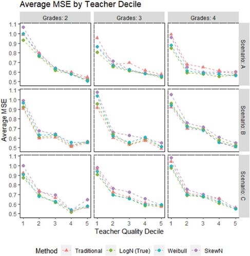
Figures 3 and 4 display bias and MSE statistics by teacher quality deciles, respectively. Though each trial draws a unique set of teachers, binning teachers across trials by true quality can reveal patterns in model performance across the spectrum of quality. For example, bias is demonstrably negatively linear with teacher ability. Negative linear bias is typical of attenuated or weakly correlated predictors; consider a zero-correlation predictor would also display negative linear bias. At the same time, this suggests that model outperformance typically happens at the margins and every method can comparably estimate teachers near the middle of the spectrum. This partially explains why the methods were less distinguishable on proportion of correctly identified quartiles versus correlation with true quality. At the extremes of teacher quality, even large disagreements between methods in teacher quality estimates are unlikely to translate into differences in quartile identification.

Fig. 3 The average bias across all trials for teachers in each decile of true quality. Teacher estimates were standardized within each method before calculating bias. Note that for visual clarity, the figure does not display the 6th to the 10th decile, as they presented essentially redundant information.

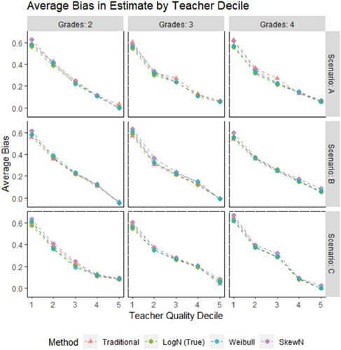
Fig. 4 The average MSE across all trials for teachers in each decile of true quality. Teacher estimates were standardized within each method before calculating MSE. Note that for visual clarity, the figure does not display the 6th to the 10th decile, as they presented essentially redundant information.

The results of this section should be narrowly interpreted with respect to the specific data generating processes used to simulate the data. By construction student-teacher assignments were completely random with full mixing. And though the distributions were somewhat based on results from empirical observations, any particular dataset may be so different as to contradict the conclusions drawn here. For example, even if the student parameter invariance assumption held, that is, the A-scenarios, if student parameters varied minimally, the marginal benefit of attending to student parameters may be insubstantial and thus be offset by the model’s increased instability from managing the additional parameters, more resembling B-scenarios.

6 Empirical Data

I use publicly available data from the National Center for Teacher Effectiveness (NCTE) to evaluate the signal-weighted value-added model for practical applications. Across the 2010–2011, 2011–2012, and 2012–2013 school years, the NCTE administered a proprietary standardized exam based on Common Core math standards to fourth and fifth graders at the end of the school year across four school districts in three states. In addition to student scores from the current and prior school year, the data also contains demographic variables at the student and teacher level for approximately 50 schools and 300 classrooms. Most importantly for the implementation of SW VAMs, the NCTE tracked classroom teacher assignments across years for each student.

In contrast to the simulation portion of this article, true teacher quality is unknowable in practice. Metrics of recovering the truth, such as correlations with true quality and correctly identified quality quartiles, are impossible to calculate. Instead, the purpose of this section is to demonstrate the viability of SW VAMs in practice, quantify the level of disagreement between the traditional and the proposed model, and compare models using reliability as measured by stability across time as a proxy for model performance. As in the simulation studies, I run the signal-weighted model three separate times specifying log normal, Weibull, and skew normal priors on student parameter distributions.

I conduct a two-step model for the estimation procedure, as in Equations (1)(1) $$Y_{\mathit{ijt}}={\beta }_0+Y_{\mathit{ijt}-1}{\beta }_1+X_{\mathit{ijt}}{\beta }_2+{\gamma }_{\mathit{ijt}}$$(1) and (2)(2) $${\gamma }_{\mathit{ijt}}=\sum _{j=1}^N{I}_{\mathit{ijt}}{\theta }_j+{\mathrm{ϵ}}_{\mathit{ijt}}$$(2) . In the first step, I regress student outcomes on prior year outcomes, grade, race/ethnicity, gender, limited English proficiency, free or reduced-price lunch status, and special education status. In the second step, I apply the value-added models on the residuals calculated in the first step to produce teacher quality estimates. Prior year outcomes were available even for observations in the 2010–2011 school year. When subsetted to students with the necessary covariates, the dataset contains 7873 unique students and 243 unique teachers.

Note that though the dataset tracks students across time, many students only appear once in the dataset. Across the three available school years and two observed grades, the data contains students from four distinct cohorts (i.e., entered fourth grade in 2009, 2010, 2011, or 2012), but contains both fourth grade and fifth grade outcomes for only two of these cohorts (i.e., entered fourth grade in 2010 or 2011).

7 Empirical Results

The traditional VAM estimates and the three sets of SW VAM estimates generally had high agreement across teachers, as shown in the correlation matrix in Table 4, but some meaningful differences did exist. To assess how these estimate differences could manifest in policy contexts, I approximate the IMPACT program policy’s performance categories and define cutoffs according to the reported distributional proportions (3%, 14%, 69% and 14%). Figure 5 plots the suggested performance categories by estimation method for all teachers arranged by their traditional VAM estimate. The traditional model disagreed on the categories of 14, 12, and 12 teachers with the log normal, Weibull, and skew normal versions of the signal-weighted model. No teachers’ quartile assignments differed by more than one, but even one quartile differences can be consequential in practice. During the IMPACT program, the highest performing category was rewarded with bonuses and base-pay salary increases. Teachers in the second lowest category faced threat of dismissal if they did not reach the top two categories in the next year. Teachers in the bottom category were immediately dismissed. For this dataset, the log normal and traditional models disagreed on a quarter of the teachers identified for immediate dismissal.

Fig. 5 Teacher performance categories according to each of the models. Teachers are arranged from lowest to highest quality in order of the estimate suggested by the traditional model. Performance categories were defined cutoffs corresponding to the 3${}^{\text{rd}}$, 17${}^{\text{th}}$, 86${}^{\text{th}}$, and 100${}^{\text{th}}$ percentile within each method’s teacher estimates.

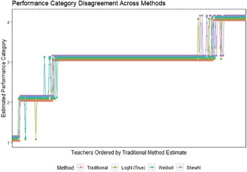
Table 4 Correlation matrix across methods of the NCTE teacher estimates.

	Traditional	Log normal	Weibull	Skew normal
Traditional	1.000	0.985	0.993	0.989
Log normal	0.985	1.000	0.993	0.973
Weibull	0.993	0.993	1.000	0.981
Skew normal	0.989	0.973	0.981	1.000

Though we cannot directly assess each model’s ability to recover true teach quality on this empirical data, we can compare estimate stability across time within teachers. As mentioned previously, this is a standard way to assess value-added model reliability, as greater stability of estimates across time suggests greater ability to capture the real, persistent component of teacher quality (Koedel, Mihaly, and Rockoff 2015). To calculate this, I divide the data by cohorts who entered fourth grade in 2009 or 2010, and cohorts who entered fourth grade in 2011 or 2012. I then run each model on each subset of data and compare the estimates for the 102 teachers present across both subsets. The correlation across cohorts for the traditional model is 0.374, while the log normal, Weibull, and skew normal version of the signal-weighted model demonstrate correlations of 0.423, 0.400, and 0.406, respectively. The IMPACT inspired performance categories are about as stable for the traditional model, 56.4% performance category agreement across cohorts, whereas the log normal, Weibull, and skew normal versions had 54.5%, 55.4%, and 58.4% percent agreement.

As an exploratory venture, I use the results from the log normal specified signal-weighted model conducted on all cohorts to regress reliability and sensitivity parameters on student characteristics and find some agreement with the conclusions of Herrmann, Walsh, and Isenberg (2016). As shown in Table 5, students who receive special education services are not only less reliable signalers of teacher quality but are also less sensitive signalers. Students with lower prior achievement are less sensitive to teacher quality, but indistinguishably reliable. In addition, male students and white students produce less reliable signals on average, while African American students produce more reliable signals. I do not find any relationship between free- or reduced- price lunch status or limited English proficiency and any of the student parameters, in contrast to the cited authors. These two sets of findings do not necessarily contradict, as they were produced by two distinct modeling frameworks. A deeper investigation would be necessary to fully disentangle how data could present these characteristics simultaneously (e.g., low prior achievement students, with their lower sensitivity, do not accurately reflect average teacher quality and this manifests as larger residuals when compared to non-low prior achievement students). Furthermore, the present study has only investigated the ability of SW VAMs to recover teacher parameters, and has not yet determined the accuracy with which the model can recover individual student parameters.

Table 5 Student signal-weighted model parameters regressed on student characteristics.

Covariate (multiplied by 0.01)	a-parameter	$\alpha -$parameter
Prior Year Score	–0.358	1.811${}^{\ast \ast \ast }$
	(0.236)	(0.646)
Male	–1.421${}^{\ast \ast \ast }$	0.413
	(0.423)	(1.161)
African American	1.154${}^{\ast \ast }$	–1.079
	(0.429)	(1.175)
Hispanic	–0.215	0.417 (1.431)
	(0.522)	(1.431)
White	–1.100${}^{\ast }$	0.359
	(0.477)	(1.307)
Other	–0.606	4.791
	(1.117)	(3.062)
FRPL	0.092	–0.202
	(0.439)	(1.200)
SPED	–2.717${}^{\ast \ast \ast }$	–6.019${}^{\ast \ast }$
	(0.682)	(1.871)
LEP	0.095	1.940
	(0.571)	(1.566)

NOTE: Each covariate was regressed separately. Note each covariate was multiplied by 0.01 to rescale the resulting coefficient for visual clarity.

Standard deviations displayed in parentheses; statistical significance calculated using linear regression ${}^{\ast }p<0.05$; ${}^{\ast \ast }p<0.01$; ${}^{\ast \ast \ast }p<0.001$.

This empirical analysis conducted on the NCTE data shows that the SW VAM is viable in a real-world context, the signal-weighted models even demonstrating greater reliability across all prior distribution specifications than traditional models. Despite high overall agreement, though, the differences between the two methods raise a number of important questions. On the one hand, the fact that the models agreed to such an extent, while one ostensibly attended to individual student parameters, suggests that the common concern that traditional VAMs do not account for classroom compositions may be unnecessary. From this perspective SW VAM could serve as a validation tool for traditional VAM estimates. On the other hand, the methods still disagreed meaningfully on the evaluations of multiple teachers which, at least for the affected teachers, is substantial. Furthermore, the NCTE data had at most two observations per student, which most closely aligns, but yet still fall short, of the two grades of observation scenarios in the previous simulation sections. Conducted on a dataset with more observations per student, the SW VAMs would likely diverge more sharply from the traditional VAM’s suggested evaluations. Until future research can determine the conditions that affect the relative accuracy of the signal-weighted versus the traditional model, policymakers should consider using both and comparing the suggested results for each teacher before enacting any high stakes consequences.

8 Discussion

This article introduces the signal-weighted value-added model, a teacher value-added estimation method that leverages the repeated observations of students to estimate student parameters and differentially interpret student outcomes as signals of teacher quality. The analysis used simulated data to assess the performance of SW VAMs to estimate teacher quality relative to a traditional VAM specification. The SW VAM better recovered estimates of true teacher quality in cases where the data generating process aligned with the signal-weighted model assumption of student parameter invariance, a result which seemed to improve with more grades of observation per student and when the student parameter prior was correctly specified. When the data generating process aligned with the traditional value-added model, the traditional model significantly outperformed the signal-weighted model. In the scenarios that aligned with neither model, the results in terms of teacher quartile identification were largely similar. Using empirical data from the NCTE, the SW VAM demonstrated higher reliability than the traditional model while showing modest disagreements on teacher classifications.

The extent to which students retain their reliability and sensitivity over time, and how distinct students’ parameters are from one another, will ultimately determine how the signal-weighted model compares to the traditional model in practice. The truth is unlikely to align entirely with any of the three simulation scenarios, but previous research suggests that some student groups do manifest different levels of reliability and sensitivity (Herrmann, Walsh, and Isenberg 2016; Stacy, Guarino, and Wooldridge 2018). It is also quite simple to imagine situations where we would reasonably expect students to differ in terms of reliability or sensitivity. If a student interacts comparatively less with their teacher due to periodic absences or voluntary remote schooling a lower proportion of the student’s performance will depend on their teacher assignment (i.e., low sensitivity), a notion similar to the “dosage” teacher value-added model proposed by Isenberg and Walsh (2014).

A substantial theoretical contribution and benefit of the signal-weighted model is its compatibility with innovations from the value-added literature and the IRT literature, and to the best of this author’s knowledge, it is the first to mathematically connect the two fields to such an extent. Reckase and Martineau (2015) have suggested evaluating teachers from an IRT perspective, but only link VAMs to a 1-PL model, calculate student parameters externally to the IRT procedure, and necessarily coarsen student outcome data into a dichotomous variable. The signal-weighted model is analogous to the IRT continuous response models developed by Samejima (1973) aside from the estimation procedure and imposition of prior distributions. It can be combined with other value-added modeling variations, such as measuring school effects (Reardon and Raudenbush 2009), and additional weighting schemas (Karl, Yang, and Lohr 2013; Isenberg and Walsh 2014) and integrate common IRT considerations such as score equating (Cook and Eignor 1991), or item parameter drift (Bock, Murakl, and Pfeiffenberger 1988), both of which have suggestive parallels in the value-added context. Some concepts already have analogues in both fields: for example, multidimensional effects in VAMs (Broatch and Lohr 2012; Jackson 2018; Mulhern 2020) and multidimensional ability in IRT (Béguin and Glas 2001); and student–teacher matching in VAMs (Lockwood and McCaffrey 2009; Bates and Glick 2013; Egalite, Kisida, and Winters 2015) and differential item and test functioning in IRT (Roju, Van der Linden, and Fleer 1995; Zumbo 1999).

The analysis in this article is subject to some limitations. First, the presented metrics (identification of true quality quartile, correlation with true quality, bias and MSE by decile) only coarsely describe model performance. An alternative approach would be to simulate the same set of teachers across scenarios and trials (rather than redraw them with each trial), which could more explicitly capture model variance and uncertainty for specific units. Second, excepting number of grades of observation and underlying data generating assumptions, all the simulated datasets had identical dimensionality and drew student parameters from analogous distributions. As noted earlier, though the simulations were designed to be realistic, certain dimensions were arbitrarily set and the demonstrated results may not be valid in practical contexts which may have many more or fewer teachers, many more or fewer students per teacher, and much more or less student mixing across teachers. The focus of this paper was to stress that the SW VAM is feasible, and in fact, under certain conditions, preferable to the traditional model.

The present study suggests a number of important future investigations. Foremost, the signal-weighted value-added model should be tested on other empirical datasets. An ideal dataset to test relative performance would contain at least three grades of observation per student and, for the sake of estimating estimate stability as a proxy for reliability, contain multiple cohorts of students across the same set of teachers. A related line of inquiry is to further test the robustness of traditional VAMs versus SW VAMs to model assumption violations, particularly random assignment of students to teachers which has been perennial concern for practitioners in this field. The SW VAM, insofar as it differentiates and tracks students across grades, may be better equipped to address this dynamic. Another particularly pressing future investigation is an assessment of the method’s ability to accurately capture student parameters, a question foregone in this investigation to preserve the scope of the paper. SW VAMs by construction will yield student parameter estimates based on the assumption that such parameters are constant within students across time, and that such parameters manifest in the specified functional form. Even if model assumptions are perfectly met, given the limited number of observations per student typically available in education datasets, student parameter estimates may be too unreliable for use in any application at the individual student level. That is, the validity of SW VAMs as a method for estimating student parameters is yet unvalidated.

Finally, by introducing a value-added model designed to improve value-added estimates, the present study might appear to have presupposed the validity of using teacher VAMs to evaluate teachers and inform teacher policy. This is not the case. Insofar as policymakers already use value-added models to evaluate teachers, a plausibly more accurate model would at least make expectations of teachers clearer and performance evaluations less subject to random error. On the contrary, the signal-weighted model, as an attempt to account for student differences, directly considers validity by examining the traditional model’s susceptibility to student differences. The SW VAM, by explicitly framing value-added models as a test of teachers which measures teaching ability by using students as test items and student performance as item responses, also brings to bear measurement related validity concerns. From the perspective of a test, teacher value-added models contain some concerning characteristics, including mutually exclusive item sets, a lack of item calibration, drift in examinee ability, and the possibility for examinee performance to impact an item’s parameters. The signal- weighted value-added model proposed in this study does not by itself resolve these validity concerns. However, it does offer a statistical foundation by which to attend to student differences, examine these threats to validity, highlight overlaps between value-added and psychometric literature, and contribute to our continuing understanding of the potential of value-added models.

References

- Amrein-Beardsley, A., and Close, K. (2019), “Teacher-Level Value-Added Models on Trial: Empirical and Pragmatic Issues of Concern across Five Court Cases,” Educational Policy, 0895904819843593. DOI: 10.1177/0895904819843593.
- Amrein-Beardsley, A., and Collins, C. (2012), “The SAS education value-added assessment system (SAS[textregistered] EVAAS[textregistered]) in the Houston Independent School District (HISD): Intended and unintended consequences,” Education Policy Analysis Archives/Archivos Analíticos de Políticas Educativas, 20, 1–28.
- Bacher-Hicks, A., and de la Campa, E. (2020), “The Impact of New York City’s Stop and Frisk Program on Crime: The Case of Police Commanders,” Available at https://drive.google.com/file/d/1SxbK9/_9mPwopEGyAyvJ606jrqCL1rwxT/view. Accessed November 4, 2020.
- Bates, L. A., and Glick, J. E. (2013), “Does it Matter if Teachers and Schools Match the Student? Racial and Ethnic Disparities in Problem Behaviors,” Social Science Research, 42, 1180–1190. DOI: 10.1016/j.ssresearch.2013.04.005.
- Béguin, A. A., and Glas, C. A. (2001), “MCMC Estimation and Some Model-Fit Analysis of Multidimensional IRT Models,” Psychometrika, 66, 541–561. DOI: 10.1007/BF02296195.
- Bock, R. D., Murakl, E., and Pfeiffenberger, W. (1988), “Item pool maintenance in the presence of item parameter drift,” Journal of Educational Measurement, 25, 275–285. DOI: 10.1111/j.1745-3984.1988.tb00308.x.
- Broatch, J., and Lohr, S. (2012), “Multidimensional Assessment of Value Added by Teachers to Real-World Outcomes,” Journal of Educational and Behavioral Statistics, 37, 256–277. DOI: 10.3102/1076998610396900.
- Chetty, R., Friedman, J. N., and Rockoff, J. E. (2014), “Measuring the Impacts of Teachers II: Teacher Value-added and Student Outcomes in Adulthood,” American Economic Review, 104, 2633–2679. DOI: 10.1257/aer.104.9.2633.
- Chetty, R., Friedman, J., Hilger, N., Saez, E., Schanzenbach, D. W., and Yagan, D. (2011), “How Does your Kindergarten Classroom Affect your Earnings? Evidence from Project Star,” The Quarterly Journal of Economics, 126, 1593–1660. DOI: 10.1093/qje/qjr041.
- Close, K., Amrein-Beardsley, A., and Collins, C. (2019), “Mapping America’s Teacher Evaluation Plans under ESSA,” Phi Delta Kappan, 101, 22–26. DOI: 10.1177/0031721719879150.
- Cook, L. L., and Eignor, D. R. (1991), “IRT Equating Methods,” Educational Measurement: Issues and Practice, 10, 37–45. DOI: 10.1111/j.1745-3992.1991.tb00207.x.
- Dee, T. S., and Wyckoff, J. (2015), “Incentives, Selection, and Teacher Performance: Evidence from IMPACT,” Journal of Policy Analysis and Management, 34, 267–297. DOI: 10.1002/pam.21818.
- Egalite, A. J., Kisida, B., and Winters, M. A. (2015), “Representation in the Classroom: The Effect of Own-race Teachers on Student Achievement,” Economics of Education Review, 45, 44–52. DOI: 10.1016/j.econedurev.2015.01.007.
- Ehlert, M., Koedel, C., Parsons, E., and Podgursky, M. (2013), “The Sensitivity of Value-added Estimates to Specification Adjustments: Evidence from School- and Teacher-level Models in Missouri,” Statistics and Public Policy, 1, 19–27. DOI: 10.1080/2330443X.2013.856152.
- Guarino, C. M., Reckase, M. D., and Wooldridge, J. M. (2015), “Can Value-added Measures of Teacher Performance be Trusted?” Education Finance and Policy, 10, 117–156. DOI: 10.1162/EDFP_a_00153.
- Harris, D., and Herrington, C. D. (2015), “Editors’ Introduction: The Use of Teacher Value-Added Measures in Schools: New Evidence, Unanswered Questions, and Future Prospects,” Educational Researcher, 44, 71–76. DOI: 10.3102/0013189X15576142.
- Herrmann, M., Walsh, E., and Isenberg, E. (2016), “Shrinkage of Value-added Estimates and Characteristics of Students with Hard-to Predict Achievement Levels,” Statistics and Public Policy, 3, 1–10. Policy Analysis Archives, 20(12), n12.
- Isenberg, E., and Walsh, E. (2014), Measuring Teacher Value Added in DC, 2013–2014 School Year. Washington, DC: Mathematica Policy Research.
- Jackson, C. K. (2018), “What do Test Scores Miss? The Importance of Teacher Effects on Non–test Score Outcomes,” Journal of Political Economy, 126, 2072–2107. DOI: 10.1086/699018.
- Kane, T. J., and Staiger, D. O. (2008). Estimating teacher impacts on student achievement: An experimental evaluation (No. w14607). National Bureau of Economic Research.
- Karl, A. T., Yang, Y., and Lohr, S. L. (2013), “A Correlated Random Effects Model for Nonignorable Missing Data in Value-added Assessment of Teacher Effects,” Journal of Educational and Behavioral Statistics, 38, 577–603. DOI: 10.3102/1076998613494819.
- Koedel, C., Mihaly, K., and Rockoff, J. E. (2015), “Value-added Modeling: A Review,” Economics of Education Review, 47, 180–195. DOI: 10.1016/j.econedurev.2015.01.006.
- Lockwood, J. R., and McCaffrey, D. F. (2009), “Exploring Student–Teacher Interactions in Longitudinal Achievement Data,” Education Finance and Policy, 4, 439–467. DOI: 10.1162/edfp.2009.4.4.439.
- Lockwood, J. R., and McCaffrey, D. F. (2014), “Correcting for Test Score Measurement Error in ANCOVA Models for Estimating Treatment Effects,” Journal of Educational and Behavioral Statistics, 39, 22–52. DOI: 10.3102/1076998613509405.
- McCaffrey, D. F., Lockwood, J. R., Koretz, D. M., Louis, T. A., and Hamilton, L. (2004), “Models for Value-added Modeling of Teacher Effects,” Journal of Educational and Behavioral Statistics, 29, 67–101. DOI: 10.3102/10769986029001067.
- Mulhern, C. (2020), “Personalized Information and College Choices: The Role of School Counselors, Technology, and Siblings,” Doctoral dissertation.
- Papay, J. P., and Kraft, M. A. (2015), “Productivity Returns to Experience in the Teacher Labor Market: Methodological Challenges and New Evidence on Long-Term Career Improvement,” Journal of Public Economics, 130, 105–119. DOI: 10.1016/j.jpubeco.2015.02.008.
- Reardon, S. F., and Raudenbush, S. W. (2009), “Assumptions of Value-added Models for Estimating School Effects,” Education, 4, 492–519.
- Reckase, M. D., and Martineau, J. A. (2015), “The Evaluation of Teachers and Schools using the Educator Response Function (ERF),” in Educator Response Function in Value Added Modeling and Growth Modeling with Particular Application to Teacher and School Effectiveness, eds. R. W. Lissitz and H. Jiao, pp. 219–236. Charlotte, NC: Information Age Publishing.
- Roju, N. S., Van der Linden, W. J., and Fleer, P. F. (1995), “IRT-based Internal Measures of Differential Functioning of Items and Tests,” Applied Psychological Measurement, 19, 353–368. DOI: 10.1177/014662169501900405.
- Rotherham, A. J., and Mitchel, A. L., (2014), Genuine Progress, Greater Challenges: A Decade of Teacher Effectiveness Reforms, Bellwether Education Partners. https://bellwethereducation.org/sites/default/files/JOYCE_Teacher%20Effectiveness_web.pdf
- Rothstein, J. (2009), “Student Sorting and Bias in Value-added Estimation: Selection on Observables and Unobservables,” Education Finance and Policy, 4, 537–571. DOI: 10.1162/edfp.2009.4.4.537.
- Samejima, F. (1973), “Homogeneous Case of the Continuous Response Model,” Psychometrika, 38, 203–219. DOI: 10.1007/BF02291114.
- Sass, T. R. (2008), “The Stability of Value-Added Measures of Teacher Quality and Implications for Teacher Compensation Policy. Brief 4.” National Center for Analysis of Longitudinal Data in Education Research.
- Stacy, B., Guarino, C., and Wooldridge, J. (2018), “Does the Precision and Stability of Value-added Estimates of Teacher Performance Depend on the Types of Students they Serve?” Economics of Education Review, 64, 50–74. DOI: 10.1016/j.econedurev.2018.04.001.
- Stan Development Team. (2018), RStan: The R Interface to Stan. R package version 2.17. 3.
- Wang, T., and Zeng, L. (1998), “Item Parameter Estimation for a Continuous Response Model Using an EM Algorithm,” Applied Psychological Measurement, 22, 333–344. DOI: 10.1177/014662169802200402.
- Zumbo, B. D. (1999), A Handbook on the Theory and Methods of Differential Item Functioning (DIF), Ottawa: National Defense Headquarters.