Adaptive control of time-delayed bilateral teleoperation systems with uncertain kinematic and dynamics

Abstract

This paper investigates the adaptive control design problem for time-delayed bilateral teleoperation systems with dynamic and kinematic uncertainties. The majority of the previous investigations in the field of teleoperation systems have only considered the dynamic uncertainties of robots. However, this research studies simultaneous adaptation to both dynamic and kinematic uncertainties. In the presented adaptive control structure, the dynamic and kinematic parameters of the robots are estimated through the proposed adaptive laws and the estimated parameters are utilized to apply amodel-based control law to the teleoperation system. The stability analysis of the teleoperation system with time delay and uncertainties in both kinematic and dynamic parameters is studied based on the Input-to-State Stability (ISS) approach. Simulation results are presented to study the performance of the proposed control structure.

Keywords:

• teleoperation systems
• dynamic uncertainty
• kinematic uncertainty
• adaptive control
• Input-to-State Stability (ISS)

PUBLIC INTEREST STATEMENT

There are two major types of uncertainties in robotic systems including the kinematic uncertainty and dynamic uncertainty. Kinematic uncertainty represents the uncertainty in the geometry of the robots, whereas dynamic uncertainty is related to the relation between the force and position of the robot. The majority of previous investigations in the field of teleoperation systems have only considered the dynamic uncertainty. This research studies adaptation to both kinematic and dynamic uncertainties by proposing stable adaptive laws. The stability of the overall system is mathematically analyzed and the effectiveness of the proposed method is illustrated through simulation results.

1. Introduction

Teleoperation systems extend the sensing and manipulation abilities of human operators to an environment, which might be remote, out-of-reach, hazardous, or virtual. Owing to this remarkable feature, these systems have found several applications in areas such as robotic surgery, space explorations, investigations on chemical materials and training simulators (Abdeetedal, Rezaee, Talebi, & Abdollahi, 2018; Iqbal, Ullah, Khan, & Irfan, 2015; Motaharifar, Talebi, Abdollahi, & Afshar, 2015). A bilateral teleoperation system consists of a master robot manipulator and a slave robot manipulator that are connected together through a communication channel (Agand, Motaharifar, & Taghirad, 2017). The motion commands exerted by the human operator to the master robot are applied to the environment through the slave robot. An important objective of the teleoperation system is the position tracking which means that the slave robot has to follow the position of the master robot. Another objective of bilateral teleoperation systems is to recreate the sense of touch with the remote environment for the operator. The most significant challenge for the control design of such systems is to ensure the stability of the overall teleoperation system with time delay. It is proven that the existence of even a small communication delay may cause the system to become unstable (Ferrell, 1966).

Up to now, numerous control architectures have been presented for teleoperation systems. The most straightforward approach is to consider the linear model of the teleoperation system as performed in (Anderson and Spong, 1989; Hashtrudi-Zaad & Salcudean, 2002; Lawrence, 1993). However, since most of the real teleoperation systems have nonlinear dynamical models, the application of such schemes is limited to only a few linear systems. In order to extend the application of control laws to a wider class of systems, several investigators have developed methodologies for control synthesis and stability analysis of teleoperation systems based on nonlinear dynamical models. For instance, the problem of controller design and stabilization of nonlinear teleoperation systems in the presence of communication time delay based on the input—to state stability (ISS) approach have been studied in Polushin and Marquez (2003). Note that, the control structure presented in (Polushin & Marquez, 2003) is limited since it supposed the dynamics of the robots to be known without any uncertainty. This assumption is, however, not realistic as in practical robotics systems the exact values of dynamic parameters are unknown. Several studies have developed control architectures to tackle the problem of dynamic uncertainty in teleoperation systems. In particular, the adaptive control methodology have been employed in (Chopra, Spong, & Lozano, 2008) and (Nuño, Ortega, & Basañez, 2010) to estimate uncertain parameters and develop model-based control laws for teleoperation systems. Note that, these studies have presented position-position control structures, meaning that the positions of each of the master and slave robots are transmitted to the other side. Generally, an accurate sense of environment is not recreated for the human operator in the position-position control scheme. Another choice which is called force reflection structure is to transmit and reflect the environment force to the master side.

Based on the force reflection control structure, several adaptive control methodologies have been developed to estimate the unknown parameters and stabilize the teleoperation system (Polushin, Liu, & Lung, 2012; Polushin, Tayebi, & Marquez, 2006; Shahdi & Sirouspour, 2009; Sharifi, Talebi, & Motaharifar, 2017). Notwithstanding the fact that those adaptive schemes have been developed for adaptation to dynamic parameters, the problem of simultaneous adaptation to both dynamic and kinematic parameters have been studied only in a few investigations. As an explanation, the kinematic uncertainty is related to the unknown parameters in the kinematic equations of the robot (Cheah, Liu, & Slotine, 2006). In order to deal with the control design problem for teleoperation systems under both kinematic and dynamic uncertainties, some studies have presented adaptive control laws that can estimate the uncertain parameters (Liu, Tavakoli, & Huang, 2010). However, the stability analysis presented in (Liu et al., 2010) did not consider the communication time delay. Notably, in the majority of real teleoperation systems, communication time delay exists as an essential component. Thus, stability analysis in the absence of time delay is incomplete.

In this research, an adaptive control approach is presented to stabilize the teleoperation system under uncertainty in both kinematic and dynamic parameters. In order to have a teleoperation system with appropriate performance, a force reflection control structure is utilized with the presented adaptive control approach. The stability of the closed-loop system in the presence of time delay and uncertainty is analyzed using the input-to-state stability (ISS) methodology. To the best of our knowledge, this is the first force reflection control structure that considers adaptation to both kinematic and dynamic uncertainties.

In summary, the main contribution of this research is to propose an adaptive control scheme for teleoperation systems, which ensures the stability of closed-loop system in the presence of both kinematics and dynamics uncertainties. Preliminary outcomes of this research were presented to an international conference (Javid & Ali Nekoui, 2018). This paper contains detailed steps of the control structure design, stability analysis in a more general case, and new simulation results.

The remainder of this paper is structured as follows: The model of the teleoperation system is illustrated in Section 2. The proposed control methodology is elaborated in Section 3. In Section 4, the stability of the system is investigated. Simulation results are presented in Section 5. Finally, the concluding remarks are stated in Section 6.

2. System description

The dynamic models of the master and slave robot manipulators are presented as (Spong, Hutchinson, & Vidyasagar, 2006) (de Wit, Siciliano, & Bastin, 2012)

(1) $M_{qm}\left(q_m\right).{\ddot{q}}_m+C_{qm}\left(q_m,{\dot{q}}_m\right).{\dot{q}}_m+g_{qm}\left(q_m\right)=U_m+J_m^T\left(q_m\right).F_h$(1)

(2) $M_{qs}\left(q_s\right).{\ddot{q}}_s+C_{qs}\left(q_s,{\dot{q}}_s\right).{\dot{q}}_s+g_{qs}\left(q_s\right)=U_s+J_s^T\left(q_s\right).F_e$(2)

where ${\mathrm{M}}_{\mathrm{q}\mathrm{m}}\left({\mathrm{q}}_{\mathrm{m}}\right),{\mathrm{M}}_{\mathrm{q}\mathrm{s}}\left({\mathrm{q}}_{\mathrm{s}}\right)\in {\mathrm{R}}^{\mathrm{n}\times \mathrm{n}}$ are the inertia matrices, ${\mathrm{C}}_{\mathrm{q}\mathrm{m}}\left(q_m,{\dot{q}}_m\right),{\mathrm{C}}_{\mathrm{q}\mathrm{s}}\left(q_s,{\dot{q}}_s\right)\in {\mathrm{R}}^{\mathrm{n}\times \mathrm{n}}$ are the matrices of Coriolis and centrifugal terms, $g_{qm}\left(q_m\right),g_{qs}\left(q_s\right)\in {\mathrm{R}}^{\mathrm{n}\times \mathrm{n}}$ are the gravity vectors, ${\mathrm{F}}_{\mathrm{h}}\in {\mathrm{R}}^{\mathrm{n}}$ is the hand force of the human operator, ${\mathrm{F}}_{\mathrm{e}}\in {\mathrm{R}}^{\mathrm{n}}$ is the environmental force, and ${\mathrm{U}}_{\mathrm{m}},{\mathrm{U}}_{\mathrm{s}}\in {\mathrm{R}}^{\mathrm{n}}$ are control laws. In the presented notations, subscripts $m$ and $s$ represent master and slave robots, respectively.

Next, some important properties of the dynamic Equations (1)(1) $M_{qm}\left(q_m\right).{\ddot{q}}_m+C_{qm}\left(q_m,{\dot{q}}_m\right).{\dot{q}}_m+g_{qm}\left(q_m\right)=U_m+J_m^T\left(q_m\right).F_h$(1) and (2(2) $M_{qs}\left(q_s\right).{\ddot{q}}_s+C_{qs}\left(q_s,{\dot{q}}_s\right).{\dot{q}}_s+g_{qs}\left(q_s\right)=U_s+J_s^T\left(q_s\right).F_e$(2) ) are reviewed (Spong et al., 2006).

Property1. The inertia matrix $M_{qi}\left(q_i\right)$,$i=m,s$ is always symmetric and positive definite for all $q_i\in {\mathbb{R}}^n$.

Property 2. The matrix ${\dot{M}}_{qi}\left(q_i,{\dot{q}}_i\right)-2C_{qi}\left(q_i,{\dot{q}}_i\right)$ is skew—symmetric; that is, for all $v\in R^n$ the following relation is true.

$v^T\left(M_{qi}\left(q_i,{\dot{q}}_i\right)-2C_{qi}\left(q_i,{\dot{q}}_i\right)\right)v=0$

Property 3. The dynamic models (1(1) $M_{qm}\left(q_m\right).{\ddot{q}}_m+C_{qm}\left(q_m,{\dot{q}}_m\right).{\dot{q}}_m+g_{qm}\left(q_m\right)=U_m+J_m^T\left(q_m\right).F_h$(1) ) and (2(2) $M_{qs}\left(q_s\right).{\ddot{q}}_s+C_{qs}\left(q_s,{\dot{q}}_s\right).{\dot{q}}_s+g_{qs}\left(q_s\right)=U_s+J_s^T\left(q_s\right).F_e$(2) ) are linear with respect to a set of physical parameters${\theta }_{{\mathrm{d}}_{\mathrm{i}}}={\left({\theta }_{{\mathrm{d}}_1},{\theta }_{{\mathrm{d}}_2},\dots \dots ,{\theta }_{{\mathrm{d}}_{\mathrm{p}}}\right)}^{\mathrm{T}}$; that is

(3) $M_{qi}\left(q_i\right).{\ddot{q}}_i+C_{qi}\left(q_i,{\dot{q}}_i\right).{\dot{q}}_i+g_{qi}\left(q_i\right)=Y_{d_i}\left(q_i,{\dot{q}}_i,{\dot{q}}_i,{\ddot{q}}_i\right).{\theta }_{d_i}$(3)

where $Y_{d_i}\left(q_i,{\dot{q}}_i,{\dot{q}}_i,{\ddot{q}}_i\right)$ is called the dynamic regressor matrix.

Then, the kinematics equations of the robots are presented as

(4) ${\mathrm{x}}_{\mathrm{i}}={\mathrm{k}}_{\mathrm{i}}\left({\mathrm{q}}_{\mathrm{i}}\right)$(4)

where $\mathrm{x}ϵ{\mathrm{R}}^{\mathrm{n}}$ is the task space vector and the nonlinear function $k_i\left(q_i\right)\text{isin}{R}^n\to R^n$ describes the relationship between the position vector in joint space and task space. Then, by differentiating both sides of (5(5) ${\dot{x}}_i=J\left(q_i\right).{\dot{q}}_i$(5) ), the relation between task space velocity ${\dot{x}}_i$ and joint space velocity ${\dot{q}}_i$ is obtained as

(5) ${\dot{x}}_i=J\left(q_i\right).{\dot{q}}_i$(5)

where $J\left(q_i\right)ϵR^{n\times n}$ is the Jacobian matrix of the robots. In order to obtain the acceleration vector in task space denoted by ${\ddot{x}}_i\text{isin}{R}^n$, Equation (6)(6) ${\ddot{x}}_i=J_i\left(q_i\right).{\ddot{q}}_i+{\dot{J}}_i\left(q_i\right).{\dot{q}}_i$(6) is differentiated as

(6) ${\ddot{x}}_i=J_i\left(q_i\right).{\ddot{q}}_i+{\dot{J}}_i\left(q_i\right).{\dot{q}}_i$(6)

Now, an important property of the kinematics of the robot manipulators is expressed.

Property4. The right-hand side of (6(6) ${\ddot{x}}_i=J_i\left(q_i\right).{\ddot{q}}_i+{\dot{J}}_i\left(q_i\right).{\dot{q}}_i$(6) ) is linear with respect to a set of kinematic parameters ${\theta }_{ki}={\left({\theta }_{k1},\dots ,{\theta }_{kq}\right)}^T$as

(7) ${\dot{x}}_i=J_i\left(q_i\right).{\dot{q}}_i=Y_{ki}\left(q_i,{\dot{q}}_i\right).{\theta }_{ki}$(7)

where ${\mathrm{Y}}_{\mathrm{k}\mathrm{i}}\left({\mathrm{q}}_{\mathrm{i}},{\dot{\mathrm{q}}}_{\mathrm{i}}\right)\in {\mathrm{R}}^{\mathrm{n}\mathrm{x}\mathrm{q}}$ is the regressor vector.

In the case that the robotic system is subject to the kinematic uncertainty, the parameters of the Jacobian matrix are not precisely known. As a result, the approximation of kinematic parameters are used to obtain an estimated value of velocity in task space as

(8) ${\hat{\dot{x}}}_i={\hat{J}}_i\left(q_i,{\hat{\theta }}_{ki}\right).{\dot{q}}_i=Y_{ki}\left(q_i,{\dot{q}}_i\right).{\hat{\theta }}_{ki}$(8)

where ${\hat{\dot{x}}}_i\in R^n$ denotes the estimated velocity vector in task space, ${\hat{J}}_i\left(q_i,{\hat{\theta }}_{ki}\right)\in R^{n\times n}$ is an approximate Jacobian matrix and ${\hat{\theta }}_{ki}\in R^q$ denotes the vector of estimated kinematic parameters.

On the other hand, the dynamics of the human operator and environment in task space are defined as the following second-order LTI models:

(9) $F_h=F_h^{\ast }-\left(M_h{\ddot{x}}_m+B_h{\dot{x}}_m+K_h{x}_m\right)$(9)

(10) $F_e=F_e^{\ast }+M_e{\ddot{x}}_s+B_e{\dot{x}}_e+K_e{x}_e$(10)

where$M_h,M_e\in {\mathrm{R}}^{\mathrm{n}\times \mathrm{n}}$ are the mass matrices, $B_h,B_e\in {\mathrm{R}}^{\mathrm{n}\times \mathrm{n}}$ are damping matrices, $K_h,K_e\in {\mathrm{R}}^{\mathrm{n}\times \mathrm{n}}$ are stiffness matrices, and $F_h^{\ast },F_e^{\ast }\in {\mathrm{R}}^{\mathrm{n}\times 1}$are the external forces.

In order to simplify the controller design and stability analysis of the teleoperation system, the dynamics of the human operator, and the environment are transformed from the task space to joint space and are combined with the dynamics of the master and slave. If Equations (4)(4) ${\mathrm{x}}_{\mathrm{i}}={\mathrm{k}}_{\mathrm{i}}\left({\mathrm{q}}_{\mathrm{i}}\right)$(4) , (5(5) ${\dot{x}}_i=J\left(q_i\right).{\dot{q}}_i$(5) ), (6(6) ${\ddot{x}}_i=J_i\left(q_i\right).{\ddot{q}}_i+{\dot{J}}_i\left(q_i\right).{\dot{q}}_i$(6) ) are substituted into (9(9) $F_h=F_h^{\ast }-\left(M_h{\ddot{x}}_m+B_h{\dot{x}}_m+K_h{x}_m\right)$(9) ) and (10(10) $F_e=F_e^{\ast }+M_e{\ddot{x}}_s+B_e{\dot{x}}_e+K_e{x}_e$(10) ) and the resulted equations are substituted into (1(1) $M_{qm}\left(q_m\right).{\ddot{q}}_m+C_{qm}\left(q_m,{\dot{q}}_m\right).{\dot{q}}_m+g_{qm}\left(q_m\right)=U_m+J_m^T\left(q_m\right).F_h$(1) ) and (2(2) $M_{qs}\left(q_s\right).{\ddot{q}}_s+C_{qs}\left(q_s,{\dot{q}}_s\right).{\dot{q}}_s+g_{qs}\left(q_s\right)=U_s+J_s^T\left(q_s\right).F_e$(2) ), the following incorporated dynamic equations are achieved:

(11) $M_m\left(q_m\right).{\ddot{q}}_m+C_m\left(q_m,{\dot{q}}_m\right).{\dot{q}}_m+g_m\left(q_m\right)=U_m+J_m^T\left(q_m\right).F_h^{\ast }$(11)

(12) $M_s\left(q_s\right).{\ddot{q}}_s+C_s\left(q_s,{\dot{q}}_s\right).{\dot{q}}_s+g_s\left(q_s\right)=U_s-J_s^T\left(q_s\right).F_e^{\ast }$(12)

where

$M_m\left(q_m\right)=M_{qm}\left(q_m\right)+J_m^T\left(q_m\right).M_h.J_m\left(q_m\right)$

$C_m\left(q_m,{\dot{q}}_m\right)=C_{qm}\left(q_m,{\dot{q}}_m\right)+J_m^T\left(q_m\right).\left(M_h.{\dot{J}}_m\left(q_m\right)+B_h.J_m\left(q_m\right)\right)$

$=C_{qm}\left(q_m,{\dot{q}}_m\right)+J_m^T\left(q_m\right).M_h.{\dot{J}}_m\left(q_m\right)+J_m^T\left(q_m\right).B_h.J_m\left(q_m\right)$

(13) $g_m\left(q_m\right)=g_{qm}\left(q_m\right)+J_m^T\left(q_m\right).K_h.{\mathrm{h}}_{\mathrm{m}}\left({\mathrm{q}}_{\mathrm{m}}\right)$(13)

$M_s\left(q_s\right)=M_{qs}\left(q_s\right)+J_s^T\left(q_s\right).M_e.J_s\left(q_s\right)$

$C_s\left(q_s,{\dot{q}}_s\right)=C_{qs}\left(q_s,{\dot{q}}_s\right)+J_s^T\left(q_s\right).\left(M_e.{\dot{J}}_s\left(q_s\right)+B_e.J_s\left(q_s\right)\right)$

$=C_{qs}\left(q_s,{\dot{q}}_s\right)+J_s^T\left(q_s\right).M_e.{\dot{J}}_s\left(q_s\right)+J_s^T\left(q_s\right).B_e.J_s\left(q_s\right)$

(14) $g_s\left(q_s\right)=g_{qs}\left(q_s\right)+J_s^T\left(q_s\right).K_e.h_s\left(q_s\right)$(14)

3. The proposed controller

First, the necessary parameters for introducing the proposed controller are explained. The parameter ${\dot{x}}_{r_i}$ for the master and slave sides are defined as

(15) ${\dot{x}}_{rm}=-{\alpha }_m.x_m$(15)

(16) ${\dot{x}}_{rs}=-{\alpha }_s.\left(x_s-x_m^d\right)$(16)

Next, (15(15) ${\dot{x}}_{rm}=-{\alpha }_m.x_m$(15) ) and (16(16) ${\dot{x}}_{rs}=-{\alpha }_s.\left(x_s-x_m^d\right)$(16) ) are differentiated with respect to time to have

(17) ${\ddot{x}}_{rm}=-{\alpha }_m.{\dot{x}}_m$(17)

(18) ${\ddot{x}}_{rs}=-{\alpha }_s.\mathrm{\Delta }{\dot{x}}_s=-{\alpha }_s.\left(\dot{x}-{\dot{x}}_m^d\right)$(18)

Then, an adaptive task—space sliding vector is defined as

(19) ${\hat{r}}_x={\hat{\dot{x}}}_i-{\dot{x}}_{ri}={\hat{J}}_i\left(q_i,{\hat{\theta }}_{ki}\right).{\dot{q}}_i-{\dot{x}}_{ri}$(19)

where ${\hat{J}}_i\left(q_i,{\hat{\theta }}_{ki}\right).{\dot{q}}_i=Y_{ki}\left(q_i,{\dot{q}}_i\right).{\hat{\theta }}_{ki}$.

Afterward, if (19(19) ${\hat{r}}_x={\hat{\dot{x}}}_i-{\dot{x}}_{ri}={\hat{J}}_i\left(q_i,{\hat{\theta }}_{ki}\right).{\dot{q}}_i-{\dot{x}}_{ri}$(19) ) is differentiated with respect to time, we have

(20) ${\hat{r}}_x={\hat{x}}_i-{\ddot{x}}_{ri}={\hat{J}}_i\left(q_i,{\hat{\theta }}_{ki}\right).{\ddot{q}}_i+{\hat{J}}_i\left(q_i,{\hat{\theta }}_{ki}\right).{\dot{q}}_i-{\ddot{x}}_{ri}$(20)

where ${\widehat{\ddot{x}}}_i$denotes the derivative of ${\hat{\dot{x}}}_i$. Next, define

(21) ${\dot{q}}_{ri}={{\hat{J}}_i}^{-1}\left(q_i,{\hat{\theta }}_{ki}\right).{\dot{x}}_{ri}$(21)

where ${{\hat{J}}_i}^{-1}\left(q_i,{\hat{\theta }}_{ki}\right)$ is the inverse of the approximate Jacobian matrix ${\hat{J}}_i\left(q_i,{\hat{\theta }}_{ki}\right)$. By differentiating (21(21) ${\dot{q}}_{ri}={{\hat{J}}_i}^{-1}\left(q_i,{\hat{\theta }}_{ki}\right).{\dot{x}}_{ri}$(21) ), we have

(22) $\begin{array}{rl}& {\ddot{q}}_{rm}={\hat{J}}_m^{-1}\left(q_m,{\hat{\theta }}_{km}\right).{\ddot{x}}_{rm}+{\hat{J}}_m^{-1}\left(q_m,{\hat{\theta }}_{km}\right).{\dot{x}}_{rm}\\ & =-{\alpha }_m.{\hat{J}}_m^{-1}\left(q_m,{\hat{\theta }}_{k_m}\right).{\dot{x}}_m-{\alpha }_m.{\hat{J}}_m^{-1}\left(q_m,{\hat{\theta }}_{k_m}\right).x_m\end{array}$(22)

(23) ${\ddot{q}}_{r_s}={\hat{J}}_s^{-1}\left(q_s,{\hat{\theta }}_{ks}\right).{\ddot{x}}_{rs}+{\hat{J}}_s^{-1}\left(q_s,{\hat{\theta }}_{ks}\right).{\dot{x}}_{rs}=-{\alpha }_s.{\hat{J}}_s^{-1}\left(q_s,{\hat{\theta }}_{ks}\right).\left({\dot{x}}_s-{\dot{x}}_m^d\right)-{\alpha }_s.{\hat{J}}_s^{-1}\left(q_s,{\hat{\theta }}_{k_s}\right).\left(x_s-x_m^d\right)$(23)

where

${\hat{J}}_m^{-1}\left(q_m,{\hat{\theta }}_{km}\right)=-{\hat{J}}_m^{-1}\left(q_m,{\hat{\theta }}_{km}\right).{\hat{J}}_m^{-1}\left(q_m,{\hat{\theta }}_{km}\right).{\hat{J}}_m^{-1}\left(q_m,{\hat{\theta }}_{km}\right)$

In order to avoid the existence of task-space velocity term in ${\ddot{q}}_{ri}$, we define

(24) $\begin{array}{rl}& {\hat{q}}_{rm}={\hat{J}}_m^{-1}\left(q_m,{\hat{\theta }}_{km}\right).{\hat{x}}_{rm}+{\hat{J}}_m^{-1}\left(q_m,{\hat{\theta }}_{km}\right).{\dot{x}}_{rm}\\ & =-{\alpha }_m.{\hat{J}}_m^{-1}\left(q_m,{\hat{\theta }}_{km}\right).{\hat{\dot{x}}}_m-{\alpha }_m.{\hat{J}}_m^{-1}\left(q_m,{\hat{\theta }}_{km}\right).x_m\end{array}$(24)

(25) $\begin{array}{rl}& {\hat{q}}_{rs}={\hat{J}}_s^{-1}\left(q_s,{\hat{\theta }}_{ks}\right).{\hat{x}}_{rs}+{\hat{J}}_s^{-1}\left(q_s,{\hat{\theta }}_{ks}\right).{\dot{x}}_{rs}\\ & =-{\alpha }_s.{\hat{J}}_s^{-1}\left(q_s,{\hat{\theta }}_{ks}\right).\left({\hat{\dot{x}}}_s-{\dot{x}}_m^d\right)-{\alpha }_s.J_s^{-1}\left(q_s,{\hat{\theta }}_{ks}\right).\left(x_s-x_m^d\right)\end{array}$(25)

where

(26) ${\hat{x}}_{rm}=-{\alpha }_m.{\hat{\dot{x}}}_m$(26)

(27) ${\hat{x}}_{rs}=-{\alpha }_s.\left({\hat{\dot{x}}}_s-{\dot{x}}_m^d\right)$(27)

From (17(17) ${\ddot{x}}_{rm}=-{\alpha }_m.{\dot{x}}_m$(17) ), (18(18) ${\ddot{x}}_{rs}=-{\alpha }_s.\mathrm{\Delta }{\dot{x}}_s=-{\alpha }_s.\left(\dot{x}-{\dot{x}}_m^d\right)$(18) ), (26(26) ${\hat{x}}_{rm}=-{\alpha }_m.{\hat{\dot{x}}}_m$(26) ), and (27(27) ${\hat{x}}_{rs}=-{\alpha }_s.\left({\hat{\dot{x}}}_s-{\dot{x}}_m^d\right)$(27) ), we have

(28) $\begin{array}{l}{\widehat{x}}_{rm}=-{\alpha }_m.{\dot{x}}_m+{\alpha }_m.{\dot{x}}_m-{\alpha }_m.{\widehat{\dot{x}}}_m\\ =-{\alpha }_m.{\dot{x}}_m+{\alpha }_m.\left({\dot{x}}_m-{\widehat{\dot{x}}}_m\right)={\ddot{x}}_{rm}+{\alpha }_m.\left({\dot{x}}_m-{\widehat{\dot{x}}}_m\right)\end{array}$(28)

(29) $\begin{array}{l}{\widehat{\ddot{x}}}_{rs}=-{\alpha }_s.\left({\dot{x}}_s-{\dot{x}}_m^d\right)+{\alpha }_s.\left({\dot{x}}_s-{\dot{x}}_m^d\right)-{\alpha }_s.\left({\widehat{\dot{x}}}_s-{\dot{x}}_m^d\right)\\ =-{\alpha }_s.\left({\dot{x}}_s-{\dot{x}}_m^d\right)+{\alpha }_s.\left({\dot{x}}_s-{\dot{x}}_m^d\right)-{\alpha }_s.\left({\widehat{\dot{x}}}_s-{\dot{x}}_m^d\right)\\ ={\ddot{x}}_{rs}+{\alpha }_s.\left({\dot{x}}_s-{\widehat{\dot{x}}}_s\right)\end{array}$(29)

Then (28(28) $\begin{array}{l}{\widehat{x}}_{rm}=-{\alpha }_m.{\dot{x}}_m+{\alpha }_m.{\dot{x}}_m-{\alpha }_m.{\widehat{\dot{x}}}_m\\ =-{\alpha }_m.{\dot{x}}_m+{\alpha }_m.\left({\dot{x}}_m-{\widehat{\dot{x}}}_m\right)={\ddot{x}}_{rm}+{\alpha }_m.\left({\dot{x}}_m-{\widehat{\dot{x}}}_m\right)\end{array}$(28) ) and (29(29) $\begin{array}{l}{\widehat{\ddot{x}}}_{rs}=-{\alpha }_s.\left({\dot{x}}_s-{\dot{x}}_m^d\right)+{\alpha }_s.\left({\dot{x}}_s-{\dot{x}}_m^d\right)-{\alpha }_s.\left({\widehat{\dot{x}}}_s-{\dot{x}}_m^d\right)\\ =-{\alpha }_s.\left({\dot{x}}_s-{\dot{x}}_m^d\right)+{\alpha }_s.\left({\dot{x}}_s-{\dot{x}}_m^d\right)-{\alpha }_s.\left({\widehat{\dot{x}}}_s-{\dot{x}}_m^d\right)\\ ={\ddot{x}}_{rs}+{\alpha }_s.\left({\dot{x}}_s-{\widehat{\dot{x}}}_s\right)\end{array}$(29) ) are substituted into (24(24) $\begin{array}{rl}& {\hat{q}}_{rm}={\hat{J}}_m^{-1}\left(q_m,{\hat{\theta }}_{km}\right).{\hat{x}}_{rm}+{\hat{J}}_m^{-1}\left(q_m,{\hat{\theta }}_{km}\right).{\dot{x}}_{rm}\\ & =-{\alpha }_m.{\hat{J}}_m^{-1}\left(q_m,{\hat{\theta }}_{km}\right).{\hat{\dot{x}}}_m-{\alpha }_m.{\hat{J}}_m^{-1}\left(q_m,{\hat{\theta }}_{km}\right).x_m\end{array}$(24) ) and (25(25) $\begin{array}{rl}& {\hat{q}}_{rs}={\hat{J}}_s^{-1}\left(q_s,{\hat{\theta }}_{ks}\right).{\hat{x}}_{rs}+{\hat{J}}_s^{-1}\left(q_s,{\hat{\theta }}_{ks}\right).{\dot{x}}_{rs}\\ & =-{\alpha }_s.{\hat{J}}_s^{-1}\left(q_s,{\hat{\theta }}_{ks}\right).\left({\hat{\dot{x}}}_s-{\dot{x}}_m^d\right)-{\alpha }_s.J_s^{-1}\left(q_s,{\hat{\theta }}_{ks}\right).\left(x_s-x_m^d\right)\end{array}$(25) ) and (22(22) $\begin{array}{rl}& {\ddot{q}}_{rm}={\hat{J}}_m^{-1}\left(q_m,{\hat{\theta }}_{km}\right).{\ddot{x}}_{rm}+{\hat{J}}_m^{-1}\left(q_m,{\hat{\theta }}_{km}\right).{\dot{x}}_{rm}\\ & =-{\alpha }_m.{\hat{J}}_m^{-1}\left(q_m,{\hat{\theta }}_{k_m}\right).{\dot{x}}_m-{\alpha }_m.{\hat{J}}_m^{-1}\left(q_m,{\hat{\theta }}_{k_m}\right).x_m\end{array}$(22) ) and (23(23) ${\ddot{q}}_{r_s}={\hat{J}}_s^{-1}\left(q_s,{\hat{\theta }}_{ks}\right).{\ddot{x}}_{rs}+{\hat{J}}_s^{-1}\left(q_s,{\hat{\theta }}_{ks}\right).{\dot{x}}_{rs}=-{\alpha }_s.{\hat{J}}_s^{-1}\left(q_s,{\hat{\theta }}_{ks}\right).\left({\dot{x}}_s-{\dot{x}}_m^d\right)-{\alpha }_s.{\hat{J}}_s^{-1}\left(q_s,{\hat{\theta }}_{k_s}\right).\left(x_s-x_m^d\right)$(23) ) are used to have

(30) ${\widehat{\ddot{q}}}_{ri}={\ddot{q}}_{ri}-{\alpha }_i.{\dot{q}}_i+{\alpha }_i.{\widehat{J}}_i{ }^{-1}\left(q_i,{\widehat{\theta }}_{ki}\right).J_i\left(q_i\right).{\dot{q}}_i$(30)

The next step is to define the adaptive sliding vector in joint space as follows:

(31) $r_i={\dot{q}}_i-{\dot{q}}_{r_i}$(31)

The sliding vector in joint space for the master and slave robots are defined as

(32) $\begin{array}{rl}& r_m={\hat{J}}_m^{-1}\left(q_m,{\hat{\theta }}_{km}\right).{\hat{\dot{x}}}_m+\alpha .{{\hat{J}}_m}^{-1}\left(q_m,{\hat{\theta }}_{km}\right).x_m\\ & ={\hat{J}}_m^{-1}\left(q_m,{\hat{\theta }}_{km}\right).\left({\hat{\dot{x}}}_m+\alpha .x_m\right)={\hat{J}}_m^{-1}\left(q_m,{\hat{\theta }}_{km}\right).\left({\hat{\dot{x}}}_m-{\dot{x}}_{rm}\right)\\ & ={{\hat{J}}_m}^{-1}\left(q_m,{\hat{\theta }}_{km}\right).{\hat{r}}_x\end{array}$(32)

(33) $\begin{array}{rl}& r_s={\hat{J}}_s^{-1}\left(q_s,{\hat{\theta }}_{k_s}\right).{\hat{\dot{x}}}_s+{\alpha }_s.{{\hat{J}}_s}^{-1}\left(q_s,{\hat{\theta }}_{k_s}\right).\left(x_s-x_m^d\right)\\ & ={\hat{J}}_s^{-1}\left(q_s,{\hat{\theta }}_{k_s}\right).\left({\hat{\dot{x}}}_s+{\alpha }_s.\left(x_s-x_m^d\right)\right)={\hat{J}}_s^{-1}\left(q_s,{\hat{\theta }}_{k_s}\right).\left({\hat{\dot{x}}}_s-{\dot{x}}_{r_s}\right)\\ & ={{\hat{J}}_s}^{-1}\left(q_s,{\hat{\theta }}_{k_s}\right).{\hat{r}}_x\end{array}$(33)

Next, the derivative of $r_i$is computed as

(34) ${\dot{r}}_i={\dot{q}}_i-{\ddot{q}}_{ri}$(34)

Then, if ${\ddot{q}}_{ri}$is substituted from (30(30) ${\widehat{\ddot{q}}}_{ri}={\ddot{q}}_{ri}-{\alpha }_i.{\dot{q}}_i+{\alpha }_i.{\widehat{J}}_i{ }^{-1}\left(q_i,{\widehat{\theta }}_{ki}\right).J_i\left(q_i\right).{\dot{q}}_i$(30) ) into (34(34) ${\dot{r}}_i={\dot{q}}_i-{\ddot{q}}_{ri}$(34) ), we have

(35) ${\dot{r}}_i={\ddot{q}}_i-\left({\widehat{\ddot{q}}}_{ri}+{\alpha }_i.{\dot{q}}_i\right)+{\alpha }_i.{\widehat{J}}_i{ }^{-1}\left(q_i,{\widehat{\theta }}_{ki}\right).J_i\left(q_i\right).{\dot{q}}_i$(35)

Afterward, (35(35) ${\dot{r}}_i={\ddot{q}}_i-\left({\widehat{\ddot{q}}}_{ri}+{\alpha }_i.{\dot{q}}_i\right)+{\alpha }_i.{\widehat{J}}_i{ }^{-1}\left(q_i,{\widehat{\theta }}_{ki}\right).J_i\left(q_i\right).{\dot{q}}_i$(35) ) and (31(31) $r_i={\dot{q}}_i-{\dot{q}}_{r_i}$(31) ) are substituted in (11(11) $M_m\left(q_m\right).{\ddot{q}}_m+C_m\left(q_m,{\dot{q}}_m\right).{\dot{q}}_m+g_m\left(q_m\right)=U_m+J_m^T\left(q_m\right).F_h^{\ast }$(11) ), to obtain

(36) $\begin{array}{l}{M}_m\left(q_m\right).\left({\dot{r}}_m+\left({\widehat{\ddot{q}}}_{rm}+{\alpha }_m.{\dot{q}}_m\right)-{\alpha }_m.{\widehat{J}}_m{ }^{-1}\left(q_m,{\widehat{\theta }}_{k_m}\right).J_m\left(q_m\right).{\dot{q}}_m\right)\\ +C_m\left(q_m,{\dot{q}}_m\right).\left(r_m+{\dot{q}}_{r_m}\right)+g_m\left(q_m\right)=U_m+J_m^T\left(q_m\right).F_h^{\text{*}}.\end{array}$(36)

Similarly, from (35(35) ${\dot{r}}_i={\ddot{q}}_i-\left({\widehat{\ddot{q}}}_{ri}+{\alpha }_i.{\dot{q}}_i\right)+{\alpha }_i.{\widehat{J}}_i{ }^{-1}\left(q_i,{\widehat{\theta }}_{ki}\right).J_i\left(q_i\right).{\dot{q}}_i$(35) ), (31(31) $r_i={\dot{q}}_i-{\dot{q}}_{r_i}$(31) ), and (12(12) $M_s\left(q_s\right).{\ddot{q}}_s+C_s\left(q_s,{\dot{q}}_s\right).{\dot{q}}_s+g_s\left(q_s\right)=U_s-J_s^T\left(q_s\right).F_e^{\ast }$(12) ), the following equation is achieved:

(37) $M_s\left(q_s\right).\left({\dot{r}}_s+\left({\widehat{\dot{q}}}_{rs}+{\alpha }_s.{\dot{q}}_s\right)-{\alpha }_s.{\widehat{J}}_s{ }^{-1}\left(q_s,{\widehat{\theta }}_{k_s}\right).J_s\left(q_s\right).{\dot{q}}_s\right)+C_s\left(q_s,{\dot{q}}_s\right).\left(r_s+{\dot{q}}_{r_s}\right)+g_s\left(q_s\right)=U_s-J_s^T\left(q_s\right).F_e^{\text{*}}$(37)

Next, after simple manipulations on (36(36) $\begin{array}{l}{M}_m\left(q_m\right).\left({\dot{r}}_m+\left({\widehat{\ddot{q}}}_{rm}+{\alpha }_m.{\dot{q}}_m\right)-{\alpha }_m.{\widehat{J}}_m{ }^{-1}\left(q_m,{\widehat{\theta }}_{k_m}\right).J_m\left(q_m\right).{\dot{q}}_m\right)\\ +C_m\left(q_m,{\dot{q}}_m\right).\left(r_m+{\dot{q}}_{r_m}\right)+g_m\left(q_m\right)=U_m+J_m^T\left(q_m\right).F_h^{\text{*}}.\end{array}$(36) ) and (37(37) $M_s\left(q_s\right).\left({\dot{r}}_s+\left({\widehat{\dot{q}}}_{rs}+{\alpha }_s.{\dot{q}}_s\right)-{\alpha }_s.{\widehat{J}}_s{ }^{-1}\left(q_s,{\widehat{\theta }}_{k_s}\right).J_s\left(q_s\right).{\dot{q}}_s\right)+C_s\left(q_s,{\dot{q}}_s\right).\left(r_s+{\dot{q}}_{r_s}\right)+g_s\left(q_s\right)=U_s-J_s^T\left(q_s\right).F_e^{\text{*}}$(37) ), the following equations are resulted

$M_m\left(q_m\right).{\dot{r}}_m+C_m\left(q_m,{\dot{q}}_m\right).r_m+M_m\left(q_m\right).{\widehat{\ddot{q}}}_{rm}$

$+C_m\left(q_m,{\dot{q}}_m\right).{\dot{q}}_{r_m}+g_m\left(q_m\right)+{\alpha }_m.M_m\left(q_m\right).{\dot{q}}_m$

$-{\alpha }_m.M_m\left(q_m\right).{{\hat{J}}_m}^{-1}\left(q_m,{\hat{\theta }}_{k_m}\right).J_m\left(q_m\right).{\dot{q}}_m$

(38) $=U_m+J_m^T\left(q_m\right).F_h^{\ast }$(38)

$M_s\left(q_s\right).{\dot{r}}_s+C_s\left(q_s,{\dot{q}}_s\right).r_s+M_s\left(q_s\right).{\widehat{\ddot{q}}}_{rs}+C_s\left(q_s,{\dot{q}}_s\right).{\dot{q}}_{rs}$

$+g_s\left(q_s\right)+{\alpha }_s.M_s\left(q_s\right).{\dot{q}}_s$

$-{\alpha }_s.M_s\left(q_s\right).{{\hat{J}}_s}^{-1}\left(q_s,{\hat{\theta }}_{ks}\right).J_s\left(q_s\right).{\dot{q}}_s$

(39) $=U_s-J_s^T\left(q_s\right).F_e^{\ast }$(39)

Afterward, Property 3 is used to express (38(38) $=U_m+J_m^T\left(q_m\right).F_h^{\ast }$(38) ) and (39(39) $=U_s-J_s^T\left(q_s\right).F_e^{\ast }$(39) ) as

$M_m\left(q_m\right).{\widehat{\ddot{q}}}_m+C_m\left(q_m,{\dot{q}}_m\right).{\dot{q}}_{rm}+g_m\left(q_m\right)+{\alpha }_m.M_m\left(q_m\right).{\dot{q}}_m$

$-{\alpha }_m.M_m\left(q_m\right).{{\hat{J}}_m}^{-1}\left(q_m,{\hat{\theta }}_{km}\right).J_m\left(q_m\right).{\dot{q}}_m$

(40) $={\overline{Y}}_{dm}\left(q_m,{\dot{q}}_m,{\dot{q}}_{rm},{\widehat{\ddot{q}}}_{rm},{\widehat{\theta }}_{km}\right).{\theta }_{dm}$(40)

$M_s\left(q_s\right).{\widehat{\ddot{q}}}_{rs}+C_s\left(q_s,{\dot{q}}_s\right).{\dot{q}}_{rs}+g_s\left(q_s\right)+{\alpha }_s.M_s\left(q_s\right).{\dot{q}}_s$

$-{\alpha }_s.M_s\left(q_s\right).{{\hat{J}}_s}^{-1}\left(q_s,{\hat{\theta }}_{k_s}\right).J_s\left(q_s\right).{\dot{q}}_s$

(41) $={\overline{Y}}_{d_s}\left(q_s,{\dot{q}}_s,{\dot{q}}_{rs},{\widehat{\ddot{q}}}_{rs},{\widehat{\theta }}_{ks}\right).{\theta }_{ds}$(41)

Then, from (40(40) $={\overline{Y}}_{dm}\left(q_m,{\dot{q}}_m,{\dot{q}}_{rm},{\widehat{\ddot{q}}}_{rm},{\widehat{\theta }}_{km}\right).{\theta }_{dm}$(40) ) and (41(41) $={\overline{Y}}_{d_s}\left(q_s,{\dot{q}}_s,{\dot{q}}_{rs},{\widehat{\ddot{q}}}_{rs},{\widehat{\theta }}_{ks}\right).{\theta }_{ds}$(41) ) it can be proved that

$M_m\left(q_m\right).{\dot{r}}_m+C_m\left(q_m,{\dot{q}}_m\right).r_m+{\overline{Y}}_{dm}\left(q_m,{\dot{q}}_m,{\dot{q}}_{rm},{\widehat{\ddot{q}}}_{rm},{\widehat{\theta }}_{km}\right).{\theta }_{dm}$

(42) $=U_m+J_m^T\left(q_m\right).F_h^{\ast }$(42)

$M_s\left(q_s\right).{\dot{r}}_s+C_s\left(q_s,{\dot{q}}_s\right).r_s+{\overline{Y}}_{ds}\left(q_s,{\dot{q}}_s,{\dot{q}}_{rs},{\widehat{\ddot{q}}}_{rs},{\widehat{\theta }}_{ks}\right).{\theta }_{ds}$

(43) $=U_s-J_s^T\left(q_s\right).F_e^{\ast }$(43)

Now, the control laws for the master and slave robots are defined as

$U_m=-{{\hat{J}}_m}^T\left(q_m,{\hat{\theta }}_{k_m}\right).\left(K_{v_m}.{\hat{\dot{x}}}_m+K_{p_m}.x_m\right)$

(44) $+{\overline{Y}}_{dm}\left(q_m,{\dot{q}}_m,{\dot{q}}_{rm},{\widehat{\ddot{q}}}_{rm},{\widehat{\theta }}_{km}\right).{\widehat{\theta }}_{d_m}+{\widehat{J}}_m^T\left(q_s\right).{\widehat{F}}_e$(44)

$U_s=-{{\hat{J}}_s}^T\left(q_s,{\hat{\theta }}_{k_s}\right).\left(K_{v_s}.{\hat{\dot{e}}}_{x_s}+K_{p_s}.e_{x_s}\right)$

(45) $+{\overline{Y}}_{ds}\left(q_s,{\dot{q}}_s,{\dot{q}}_{rs},{\widehat{\ddot{q}}}_{rs},{\widehat{\theta }}_{ks}\right).{\widehat{\theta }}_{d_s}$(45)

where $e_{x_s}=x_s-x_m^d$. Then, by substituting (44(44) $+{\overline{Y}}_{dm}\left(q_m,{\dot{q}}_m,{\dot{q}}_{rm},{\widehat{\ddot{q}}}_{rm},{\widehat{\theta }}_{km}\right).{\widehat{\theta }}_{d_m}+{\widehat{J}}_m^T\left(q_s\right).{\widehat{F}}_e$(44) ) into (42(42) $=U_m+J_m^T\left(q_m\right).F_h^{\ast }$(42) ) and (45(45) $+{\overline{Y}}_{ds}\left(q_s,{\dot{q}}_s,{\dot{q}}_{rs},{\widehat{\ddot{q}}}_{rs},{\widehat{\theta }}_{ks}\right).{\widehat{\theta }}_{d_s}$(45) ) into (43(43) $=U_s-J_s^T\left(q_s\right).F_e^{\ast }$(43) ) the closed loop system of the master and slave robots are obtained as follows:

$M_m\left(q_m\right).{\dot{r}}_m+C_m\left(q_m,{\dot{q}}_m\right).r_m+{\overline{Y}}_{d_m}\left(q_m,{\dot{q}}_m,{\dot{q}}_{rm},{\widehat{\ddot{q}}}_{rm},{\widehat{\theta }}_{k_m}\right).{\tilde{\theta }}_{dm}$

$+{\widehat{J}}_m{ }^T\left(q_m,{\widehat{\theta }}_{k_m}\right).\left(K_{v_m}.{\widehat{\dot{X}}}_m+K_{p_m}.X_m\right)$

(46) $=J_m^T\left(q_m\right).F_h^{\ast }+{\hat{J}}_m^T\left(q_s\right).{\hat{F}}_e$(46)

$M_s\left(q_s\right).{\dot{r}}_s+C_s\left(q_s,{\dot{q}}_s\right).r_s+{\overline{Y}}_{d_s}\left(q_s,{\dot{q}}_s,{\dot{q}}_{r_s},{\widehat{\ddot{q}}}_{rs},{\widehat{\theta }}_{k_s}\right).{\tilde{\theta }}_{ds}$

$+{{\hat{J}}_s}^T\left(q_s,{\hat{\theta }}_{k_s}\right).\left(K_{v_s}.\mathrm{\Delta }{\hat{\dot{x}}}_s+K_{p_s}.e_{x_s}\right)$

(47) $=J_s^T\left(q_s\right).F_e^{\ast }$(47)

where ${\tilde{\theta }}_{d_i}={\hat{\theta }}_{d_i}-{\theta }_{d_i}$. Now, the dynamic adaptation laws for the master and slave robots are described as

(48) ${\dot{\widehat{\theta }}}_{dm}=-L_d{ }_m.{\overline{Y}}_{d_m}\left(q_m,{\dot{q}}_m,{\dot{q}}_{rm},{\widehat{\ddot{q}}}_{rm},{\widehat{\theta }}_{k_m}\right).r_m-{\epsilon }_{d_m}\left({\widehat{\theta }}_{d_m}-{\theta }^{\text{*}}{ }_{d_m}\right)$(48)

(49) ${\dot{\widehat{\theta }}}_{ds}=-L_d{ }_s.{\overline{Y}}_{d_s}\left(q_s,{\dot{q}}_s,{\dot{q}}_{rs},{\widehat{\ddot{q}}}_{rs},{\widehat{\theta }}_{k_s}\right).r_s-{\epsilon }_{d_s}\left({\widehat{\theta }}_{d_s}-{\theta }^{\text{*}}{ }_{d_s}\right)$(49)

where ${{\theta }^{\ast }}_{d_m}and{{\theta }^{\ast }}_{d_s}$are the vectors of nominal dynamic parameters. Then, the following error dynamics are achieved:

(50) ${\dot{\tilde{\theta }}}_{dm}=-L_d{ }_m.{\overline{Y}}_{d_m}\left(q_m,{\dot{q}}_m,{\dot{q}}_{rm},{\widehat{\ddot{q}}}_{rm},{\widehat{\theta }}_{k_m}\right).r_m-{\epsilon }_{d_m}\left({\tilde{\theta }}_{dm}-{\tilde{\theta }}^{*}{ }_{dm}\right)$(50)

(51) ${\dot{\tilde{\theta }}}_{ds}=-L_d{ }_s.{\overline{Y}}_{d_s}\left(q_s,{\dot{q}}_s,{\dot{q}}_{rs},{\widehat{\ddot{q}}}_{rs},{\widehat{\theta }}_{k_s}\right).r_s-{\epsilon }_{d_s}\left({\tilde{\theta }}_{ds}-{\tilde{\theta }}^{*}{ }_{d_s{d}_s}\right)$(51)

where ${{\tilde{\theta }}^{\ast }}_{d_i}={{\theta }^{\ast }}_{d_i}-{\theta }_{d_i}.$ Furthermore, the adaptation laws for the kinematic parameters of the master and slave robots are defined as

${\dot{\widehat{\theta }}}_{km}=-L_{k_m}.W_{k_m}^T.K_{v_m}.\left(W_{k_m}\left(t\right).{\widehat{\theta }}_{k_m}-y_m\right)$

(52) $+L_{k_m}.Y_{k_m}^T\left(q_m,{\dot{q}}_m\right).\left(K_{p_m}+{\alpha }_m.K_{v_m}\right).x_m$(52)

${\dot{\widehat{\theta }}}_{k_s}=-L_{k_s}.W_{k_s}^T.K_{v_s}\left(W_{k_s}\left(t\right).{\widehat{\theta }}_{k_s}-y_s\right)$

(53) $+L_{k_s}.Y_{k_s}^T\left(q_s,{\dot{q}}_s\right).\left(K_{p_s}+{\alpha }_s.K_{v_s}\right).e_{x_s}$(53)

where $y_i$ is the filtered differentiation of the measured position $x_i$ and is defined as

(54) $y_i=\frac{\lambda \rho }{\rho +\lambda }.x_i=W_{k_i.}{\theta }_{k_i}$(54)

Note that, using the signal $y_i$avoids the need for measuring task space velocity. Next, the estimation error of the kinematic parameters is defined as ${\tilde{\theta }}_{k_i}={\hat{\theta }}_{k_i}-{\theta }_{k_i}$and the error dynamics are derived as

${\dot{\tilde{\theta }}}_{km}=-L_{k_m}.W_{k_m}^T.K_{v_m}\left(W_{k_m}\left(t\right).{\widehat{\theta }}_{k_m}-y_m\right)$

(55) $+L_{k_m}.Y_{k_m}^T\left(q_m,{\dot{q}}_m\right).\left(K_{p_m}+{\alpha }_m.K_{v_m}\right).x_m$(55)

${\dot{\tilde{\theta }}}_{k_s}=-L_{k_s}.W_{k_s}^T.K_{v_s}\left(W_{k_s}\left(t\right).{\widehat{\theta }}_{k_s}-y_s\right)$

(56) $+L_{k_s}.Y_{k_s}^T\left(q_s,{\dot{q}}_s\right).\left(K_{p_s}+{\alpha }_s.K_{v_s}\right)e_{x_s}$(56)

4. Stability analysis

In this section, input-to-state stability (ISS) approach is utilized to analyze the stability of the closed loop teleoperation system in the presence of kinematic and dynamic uncertainties. The definition of ISS stability is presented as follows:

Definition 1: The nonlinear system is considered as

(57) $\dot{x}=f\left(t,x,u\right)$(57)

where $f:0,\mathrm{\infty }\times R^n\times R^m\to R^n$ is piecewise continuous in $t$ and locally Lipschitz in $x$and $u$.Then, the system (58$∥x\left(t\right)∥\le \beta \left(x_0,t-t_0\right)+\gamma \left(SU{P}_{t_0\le \tau \le t}u\left(\tau \right)\right)$) is ISS, provided that a class $\mathcal{K}\mathcal{L}$ function $\beta$ and a class $\mathcal{K}$ function $\gamma$are exist such that for any initial state $x\left(t_0\right)$ and any bounded input $u\left(t\right)$, the solution $x\left(t\right)$ exist for all $t\ge t_0$ and satisfies

$∥x\left(t\right)∥\le \beta \left(x_0,t-t_0\right)+\gamma \left(SU{P}_{t_0\le \tau \le t}u\left(\tau \right)\right)$

In the next theorem, the sufficient conditions for the above definition of ISS stability based on the Lyapunov theory are presented.

Theorem 1: It is presumed that $V:\left[0,\left.\mathrm{\infty }\right)\right.\times R^n\to R$ is a continuously differentiable function such that

(59) ${\alpha }_1\left(∥x∥\right)\le V\left(t,x\right)\le {\alpha }_2\left(∥x∥\right)$(59)

(60) $\frac{\partial V}{\partial V}+\frac{\partial V}{\partial x}f\left(t,x,u\right)\le -W_3\left(x\right),\forall \Vert x\Vert \ge \rho \Vert u\Vert >0$(60)

where ${\alpha }_1,{\alpha }_2$ are class ${\mathcal{K}}_{\mathrm{\infty }}$ functions, $\rho$ is a class $\mathcal{K}$ function, and ${\mathcal{W}}_3\left(x\right)$ is a continuous positive definite function on $R^n$. Then, the system (57(57) $\dot{x}=f\left(t,x,u\right)$(57) ) is ISS with gain $\gamma ={\alpha }_1^{-1}\circ {\alpha }_2\circ \rho$.

Next, the ISS stability of the master robot is analyzed.

Proposition 1. Consider that the control law (44(44) $+{\overline{Y}}_{dm}\left(q_m,{\dot{q}}_m,{\dot{q}}_{rm},{\widehat{\ddot{q}}}_{rm},{\widehat{\theta }}_{km}\right).{\widehat{\theta }}_{d_m}+{\widehat{J}}_m^T\left(q_s\right).{\widehat{F}}_e$(44) ) and adaptation laws (48(48) ${\dot{\widehat{\theta }}}_{dm}=-L_d{ }_m.{\overline{Y}}_{d_m}\left(q_m,{\dot{q}}_m,{\dot{q}}_{rm},{\widehat{\ddot{q}}}_{rm},{\widehat{\theta }}_{k_m}\right).r_m-{\epsilon }_{d_m}\left({\widehat{\theta }}_{d_m}-{\theta }^{\text{*}}{ }_{d_m}\right)$(48) ) and (52(52) $+L_{k_m}.Y_{k_m}^T\left(q_m,{\dot{q}}_m\right).\left(K_{p_m}+{\alpha }_m.K_{v_m}\right).x_m$(52) ) are applied to the master robot. Then, the resulted closed loop system is ISS with state ${\left[{\mathrm{q}}_{\mathrm{m}}^{\mathrm{T}},{\dot{\mathrm{q}}}_{\mathrm{m}}^{\mathrm{T}},{\tilde{\theta }}_{{\mathrm{d}}_{\mathrm{m}}}^{\mathrm{T}},{\tilde{\theta }}_{{\mathrm{k}}_{\mathrm{m}}}^{\mathrm{T}}\right]}^{\mathrm{T}}$and input ${\left[{\mathrm{F}}_{\mathrm{h}}^{\mathrm{T}},{\hat{\mathrm{F}}}_{\mathrm{e}}^{\mathrm{T}},{{\tilde{\theta }}^{\ast }}_{{\mathrm{d}}_{\mathrm{m}}}^{\mathrm{T}}\right]}^{\mathrm{T}}$.

Proof: The following Lyapunov function candidate is considered:

(61) $\begin{array}{rl}& V_m=\frac{1}{2}.r_m^T.M_m\left(q_m\right).r_m+\frac{1}{2}.{\tilde{\theta }}_{d_m}^T.L_{d_m}^{-1}.{\tilde{\theta }}_{d_m}\\ & +\frac{1}{2}.{\tilde{\theta }}_{k_m}^T.L_{k_m}^{-1}.{\tilde{\theta }}_{k_m}+\frac{1}{2}.x_m^T.\left(K_{p_m}+{\alpha }_m.K_{v_m}\right).x_m\end{array}$(61)

where $\mathrm{\Delta }{\theta }_{k_m}={\bar{\theta }}_{k_m}-{\hat{\theta }}_{k_m}$. Differentiating with respect to time and using property 1, we have

$\begin{array}{l}\frac{d{V}_m}{dt}=r_m^T.M_m\left(q_m\right).{\dot{r}}_m+\frac{1}{2}.r_m^T.{\dot{M}}_m\left(q_m\right).r_m\\ -\Delta {\theta }_{d_m}^T.L_{d_m}^{-1}.{\dot{\widehat{\theta }}}_{d_m}-\Delta {\theta }_{k_m}^T.L_{k_m}^{-1}.{\dot{\widehat{\theta }}}_{k_m}\\ +x_m^T.\left(K_{p_m}+{\alpha }_m.K_{v_m}\right).{\dot{x}}_m\end{array}$

Substituting $M_m\left(q_m\right).{\dot{r}}_m$ from (42(42) $=U_m+J_m^T\left(q_m\right).F_h^{\ast }$(42) ), ${\dot{\widehat{\theta }}}_{d_m}$from (48(48) ${\dot{\widehat{\theta }}}_{dm}=-L_d{ }_m.{\overline{Y}}_{d_m}\left(q_m,{\dot{q}}_m,{\dot{q}}_{rm},{\widehat{\ddot{q}}}_{rm},{\widehat{\theta }}_{k_m}\right).r_m-{\epsilon }_{d_m}\left({\widehat{\theta }}_{d_m}-{\theta }^{\text{*}}{ }_{d_m}\right)$(48) ), and ${\dot{\widehat{\theta }}}_{k_m}$from (52(52) $+L_{k_m}.Y_{k_m}^T\left(q_m,{\dot{q}}_m\right).\left(K_{p_m}+{\alpha }_m.K_{v_m}\right).x_m$(52) ) into (62$\begin{array}{l}\frac{d{V}_m}{dt}=r_m^T.M_m\left(q_m\right).{\dot{r}}_m+\frac{1}{2}.r_m^T.{\dot{M}}_m\left(q_m\right).r_m\\ -\Delta {\theta }_{d_m}^T.L_{d_m}^{-1}.{\dot{\widehat{\theta }}}_{d_m}-\Delta {\theta }_{k_m}^T.L_{k_m}^{-1}.{\dot{\widehat{\theta }}}_{k_m}\\ +x_m^T.\left(K_{p_m}+{\alpha }_m.K_{v_m}\right).{\dot{x}}_m\end{array}$), and using property 2, we have

(63) $\begin{array}{l}\frac{d{V}_m}{dt}=-{\widehat{r}}_x{ }^T.K_{v_m}.{\widehat{\dot{x}}}_m-{\widehat{r}}_x{ }^T.K_{p_m}.x_m\\ -\Delta {\theta }_{k_m}^T.W_{k_m}^T.K_{v_m}.W_{k_m}\left(t\right).\Delta {\theta }_{k_m}+r_m^T.\left(J_m^T\left(q_m\right).F_h^{\text{*}}+{\widehat{J}}_m^T\left(q_s\right).{\widehat{F}}_e\right)\\ +\Delta {\theta }_{d_m}^T.L_{d_m}^{-1}.{\epsilon }_m.\left({\widehat{\theta }}_m-{\theta }^{\text{*}}{ }_m\right)\\ -\Delta {\theta }_{k_m}^T.L_{k_m}^{-1}.L_{k_m}.Y_{k_m}^T\left(q_m,{\dot{q}}_m\right).\left(K_{p_m}+{\alpha }_m.K_{v_m}\right).x_m\\ +x_m^T.\left(K_{p_m}+{\alpha }_m.K_{v_m}\right).{\dot{x}}_m\end{array}$(63)

On the other hand, from (19(19) ${\hat{r}}_x={\hat{\dot{x}}}_i-{\dot{x}}_{ri}={\hat{J}}_i\left(q_i,{\hat{\theta }}_{ki}\right).{\dot{q}}_i-{\dot{x}}_{ri}$(19) ), (4(4) ${\mathrm{x}}_{\mathrm{i}}={\mathrm{k}}_{\mathrm{i}}\left({\mathrm{q}}_{\mathrm{i}}\right)$(4) ) and (15(15) ${\dot{x}}_{rm}=-{\alpha }_m.x_m$(15) ) it can be verified that

(64) ${\hat{r}}_{x_m}={\dot{x}}_m+{\alpha }_m.x_m-Y_{k_m}\left(q_m,{\dot{q}}_m\right).\mathrm{\Delta }{\theta }_{k_m}$(64)

where

$Y_{k_m}\left(q_m,{\dot{q}}_m\right).\mathrm{\Delta }{\theta }_{k_m}=J_m\left(q_m\right).{\dot{q}}_m-{\hat{J}}_m\left(q_m,{\hat{\theta }}_{k_m}\right).{\dot{q}}_m$

(64) $={\dot{x}}_m-{\hat{\dot{x}}}_m$(64)

Using (63(63) $\begin{array}{l}\frac{d{V}_m}{dt}=-{\widehat{r}}_x{ }^T.K_{v_m}.{\widehat{\dot{x}}}_m-{\widehat{r}}_x{ }^T.K_{p_m}.x_m\\ -\Delta {\theta }_{k_m}^T.W_{k_m}^T.K_{v_m}.W_{k_m}\left(t\right).\Delta {\theta }_{k_m}+r_m^T.\left(J_m^T\left(q_m\right).F_h^{\text{*}}+{\widehat{J}}_m^T\left(q_s\right).{\widehat{F}}_e\right)\\ +\Delta {\theta }_{d_m}^T.L_{d_m}^{-1}.{\epsilon }_m.\left({\widehat{\theta }}_m-{\theta }^{\text{*}}{ }_m\right)\\ -\Delta {\theta }_{k_m}^T.L_{k_m}^{-1}.L_{k_m}.Y_{k_m}^T\left(q_m,{\dot{q}}_m\right).\left(K_{p_m}+{\alpha }_m.K_{v_m}\right).x_m\\ +x_m^T.\left(K_{p_m}+{\alpha }_m.K_{v_m}\right).{\dot{x}}_m\end{array}$(63) ), (64(64) ${\hat{r}}_{x_m}={\dot{x}}_m+{\alpha }_m.x_m-Y_{k_m}\left(q_m,{\dot{q}}_m\right).\mathrm{\Delta }{\theta }_{k_m}$(64) ), and (65(64) $={\dot{x}}_m-{\hat{\dot{x}}}_m$(64) ) we have

$\frac{d{V}_m}{dt}=-{\dot{x}}_m^T.K_{v_m}.{\dot{x}}_m+2{\dot{x}}_m^T.K_{v_m}{Y}_{k_m}\left(q_m,{\dot{q}}_m\right).\mathrm{\Delta }{\theta }_{k_m}$

$-\mathrm{\Delta }{\theta }_{k_m}^T.Y_{k_m}^T\left(q_m.{\dot{q}}_m\right).K_{v_m}.Y_{k_m}\left(q_m,{\dot{q}}_m\right).\mathrm{\Delta }{\theta }_{k_m}$

$-{\alpha }_m.x_m^T.K_{p_m}.x_m-\mathrm{\Delta }{\theta }_{k_m}^T.W_{k_m}^T.K_{v_m}.W_{k_m}\left(t\right).\mathrm{\Delta }{\theta }_{k_m}$

(66) $+r_m^T.\left(J_m^T\left(q_m\right).F_h^{\ast }+{\hat{J}}_m^T\left(q_s\right).{\hat{F}}_e\right)+\mathrm{\Delta }{\theta }_{d_m}^T.L_{d_m}^{-1}.{\epsilon }_m.\left({\hat{\theta }}_m-{{\theta }^{\ast }}_m\right)$(66)

Since ${\hat{\dot{x}}}_m={\dot{x}}_m-Y_{k_m}\left(q_m,{\dot{q}}_m\right).\mathrm{\Delta }{\theta }_{k_m}$, the above equation can be simplified to

$\frac{d{V}_m}{dt}=-{\hat{\dot{x}}}_m^T.K_{v_m}.{\hat{\dot{x}}}_m-{\alpha }_m.x_m^T.K_{p_m}.x_m$

$-\mathrm{\Delta }{\theta }_{k_m}^T.W_{k_m}^T.K_{v_m}.W_{k_m}\left(t\right).\mathrm{\Delta }{\theta }_{k_m}+r_m^T.\left(J_m^T\left(q_m\right).F_h^{\ast }+{\hat{J}}_m^T\left(q_s\right).{\hat{F}}_e\right)$

(67) $+\mathrm{\Delta }{\theta }_{d_m}^T.L_{d_m}^{-1}.{\epsilon }_m.\left({\hat{\theta }}_m-{{\theta }^{\ast }}_m\right)$(67)

Then, by considering that the norm of Jacobian matrix has the upper bounded ${\zeta }_{\mathrm{m}}$, the Young’s quadratic inequality is utilized to derive

$\frac{d{V}_m}{dt}\le -\left(\frac{3}{4}\right).{\lambda }_{\mathrm{m}\mathrm{i}\mathrm{n}}\left({\mathrm{k}}_{{\mathrm{v}}_{\mathrm{m}}}\right).{{\widehat{\dot{\mathrm{x}}}}_{\mathrm{m}}}^2-\left(\frac{3}{4}\right){\alpha }_{\mathrm{m}}.{\lambda }_{\mathrm{m}\mathrm{i}\mathrm{n}}\left({\mathrm{k}}_{{\mathrm{p}}_{\mathrm{m}}}\right).{{\mathrm{x}}_{\mathrm{m}}}^2$

$-\left(\frac{3}{4}\right).{\epsilon }_{\mathrm{m}}.{\lambda }_{\mathrm{m}\mathrm{i}\mathrm{n}}\left({\mathrm{L}}_{{\mathrm{d}}_{\mathrm{m}}}^{-1}\right).{{\tilde{\theta }}_{{\mathrm{d}}_{\mathrm{m}}}}^2-{\mathrm{W}}_{{\mathrm{k}}_{\mathrm{m}}}^{\mathrm{T}}\left(\mathrm{t}\right).{\mathrm{W}}_{{\mathrm{k}}_{\mathrm{m}}}\left(\mathrm{t}\right).{\lambda }_{\mathrm{m}\mathrm{i}\mathrm{n}}\left({\mathrm{k}}_{{\mathrm{v}}_{\mathrm{m}}}\right).{{\tilde{\theta }}_{{\mathrm{k}}_{\mathrm{m}}}}^2$

$+\left({{\hat{\mathrm{J}}}_{\mathrm{m}}}^{-1}{\left({\mathrm{q}}_{\mathrm{m}},{\hat{\theta }}_{{\mathrm{k}}_{\mathrm{m}}}\right)}^2.{\zeta }_{\mathrm{m}}{\mathrm{F}}_{\mathrm{h}}+{{\hat{\mathrm{F}}}_{\mathrm{e}}}^2\right).\left(\frac{1}{{\lambda }_{\mathrm{m}\mathrm{i}\mathrm{n}}\left({\mathrm{k}}_{{\mathrm{v}}_{\mathrm{m}}}\right)}+\frac{1}{{\lambda }_{\mathrm{m}\mathrm{i}\mathrm{n}}\left({\mathrm{k}}_{{\mathrm{p}}_{\mathrm{m}}}\right)}\right)$

(68) $+\left(\frac{1}{{\epsilon }_m.{\lambda }_{min}\left(L_{d_m}^{-1}\right)}.{\left|L_{d_m}^{-1}.{\epsilon }_m.{\theta }_m^{\ast }\right|}^2\right)$(68)

which shows the ISS stability of master robot. □

The next step is to study the ISS stability of slave robot as considered in Proposition 2.

Proposition 2. If the control law (45(45) $+{\overline{Y}}_{ds}\left(q_s,{\dot{q}}_s,{\dot{q}}_{rs},{\widehat{\ddot{q}}}_{rs},{\widehat{\theta }}_{ks}\right).{\widehat{\theta }}_{d_s}$(45) ) and the adaptation laws (49(49) ${\dot{\widehat{\theta }}}_{ds}=-L_d{ }_s.{\overline{Y}}_{d_s}\left(q_s,{\dot{q}}_s,{\dot{q}}_{rs},{\widehat{\ddot{q}}}_{rs},{\widehat{\theta }}_{k_s}\right).r_s-{\epsilon }_{d_s}\left({\widehat{\theta }}_{d_s}-{\theta }^{\text{*}}{ }_{d_s}\right)$(49) ) and (53(53) $+L_{k_s}.Y_{k_s}^T\left(q_s,{\dot{q}}_s\right).\left(K_{p_s}+{\alpha }_s.K_{v_s}\right).e_{x_s}$(53) ) are applied to the slave robot; then, the closed-loop system is ISS with state ${\left[q_s^T,{\dot{q}}_s^T,{\tilde{\theta }}_{d_s}^T,{\tilde{\theta }}_{k_s}^T\right]}^T$ and input ${\left[x_m^{d^T},F_e^T,{{\tilde{\theta }}^{\ast }}_{d_s}^T\right]}^T$.

Proof: The Lyapunov function candidate for the slave robot is defined as

(69) $V_s=\frac{1}{2}.r_s^T.M_s\left(q_s\right).r_s+\frac{1}{2}.{\tilde{\theta }}_{d_s}^T.L_{d_s}^{-1}.{\tilde{\theta }}_{d_s}+\frac{1}{2}.{\tilde{\theta }}_{k_s}^T.L_{k_s}^{-1}.{\tilde{\theta }}_{k_s}+\frac{1}{2}.e_{x_s}^T.\left(K_{p_s}+{\alpha }_s.K_{v_s}\right).e_{x_s}$(69)

In a similar way done for to the master robot, it may be shown that

$\frac{d{V}_s}{dt}\le -\frac{3}{4}{\lambda }_{min}\left(k_{v_s}\right).\mathrm{\Delta }{{\hat{\dot{x}}}_s}^2-{\alpha }_s.{\lambda }_{min}\left(k_{p_s}\right).\mathrm{\Delta }{x_s}^2$

$-\frac{3}{4}{\epsilon }_s.{\lambda }_{min}\left(L_{d_s}^{-1}\right).{{\tilde{\theta }}_{d_s}}^2$

$-W_{k_s}^T\left(t\right).W_{k_s}\left(t\right).{\lambda }_{min}\left(K_{v_s}\right).{\tilde{\theta }}_{k_s}{ }^2+{\alpha }_s.K_{p_s}.x{}_m^{d}2+$

$+\left(\frac{\hat{J}{{ }_s^{-1}}^T{\left(q_s,{\hat{\theta }}_{k_s}\right)}^2}{{\lambda }_{min}\left(k_{v_s}\right)}+\frac{\hat{J}{{ }_s^{-1}}^T\left(q_s,{\hat{\theta }}_{k_s}\right){.}^2}{{\lambda }_{min}\left(k_{p_s}\right)}\right){F_e}^2$

(70) $+\left(\frac{1}{{\epsilon }_m.{\lambda }_{min}\left(L_{d_m}^{-1}\right)}.{\left|L_{d_m}^{-1}.{\epsilon }_m.{\theta }_m^{\ast }\right|}^2\right)$(70)

From the relations (69(69) $V_s=\frac{1}{2}.r_s^T.M_s\left(q_s\right).r_s+\frac{1}{2}.{\tilde{\theta }}_{d_s}^T.L_{d_s}^{-1}.{\tilde{\theta }}_{d_s}+\frac{1}{2}.{\tilde{\theta }}_{k_s}^T.L_{k_s}^{-1}.{\tilde{\theta }}_{k_s}+\frac{1}{2}.e_{x_s}^T.\left(K_{p_s}+{\alpha }_s.K_{v_s}\right).e_{x_s}$(69) ) and (70(70) $+\left(\frac{1}{{\epsilon }_m.{\lambda }_{min}\left(L_{d_m}^{-1}\right)}.{\left|L_{d_m}^{-1}.{\epsilon }_m.{\theta }_m^{\ast }\right|}^2\right)$(70) ), the ISS stability of slave robot is proved. □

Now, a useful proposition regarding the ISS stability of a general system subject to input delay is presented.

Proposition 3(Ferrell, 1966). Consider that the system

$\dot{x}\left(t\right)=f\left(x\left(t\right),u\left(t\right),v\left(t\right)\right)$

is ISS with state $x\left(t\right)$ and input ${\left[u{\left(t\right)}^T,v{\left(t\right)}^T\right]}^T$. Then, the system with input delay $T_d$defined as

$\dot{x}\left(t\right)=f\left(x\left(t\right),u\left(t-T_d\right),v\left(t\right)\right)$

is also ISS with state $x\left(t\right)$ and input ${\left[u{\left(t-T_d\right)}^T,v{\left(t\right)}^T\right]}^T$.

Next, a proposition regarding the stability of a general cascade system as a tool for our final conclusion is expressed.

Proposition 4 (Ferrell, 1966). It is presumed that the system

$\dot{z}\left(t\right)=F_1\left(z_d\left(t\right),u_d\left(t\right),w_d\left(t\right)\right)$

is ISS with respect to inputs$uandw$, and the system

$\dot{y}\left(t\right)=F_2\left(y_d\left(t\right),v_d\left(t\right)\right)$

is ISS with respects to input $v$. Then, the cascade system

$\left\{\begin{array}{c}\dot{z}\left(t\right)=F_1\left(z_d\left(t\right),u_d\left(t\right),w_d\left(t\right)\right)\\ \dot{y}\left(t\right)=F_2\left(y_d\left(t\right),v_d\left(t\right)\right)\end{array}\right.$

is ISS with respect to inputs $vandw$.

Finally, the stability of overall system as our main result of this section is presented.

Theorem 2. The teleoperation system composed of the master robot with dynamic model (1(1) $M_{qm}\left(q_m\right).{\ddot{q}}_m+C_{qm}\left(q_m,{\dot{q}}_m\right).{\dot{q}}_m+g_{qm}\left(q_m\right)=U_m+J_m^T\left(q_m\right).F_h$(1) ) and the slave robot with dynamic model (2(2) $M_{qs}\left(q_s\right).{\ddot{q}}_s+C_{qs}\left(q_s,{\dot{q}}_s\right).{\dot{q}}_s+g_{qs}\left(q_s\right)=U_s+J_s^T\left(q_s\right).F_e$(2) ) with the control inputs (44(44) $+{\overline{Y}}_{dm}\left(q_m,{\dot{q}}_m,{\dot{q}}_{rm},{\widehat{\ddot{q}}}_{rm},{\widehat{\theta }}_{km}\right).{\widehat{\theta }}_{d_m}+{\widehat{J}}_m^T\left(q_s\right).{\widehat{F}}_e$(44) ) and (45(44) $+{\overline{Y}}_{dm}\left(q_m,{\dot{q}}_m,{\dot{q}}_{rm},{\widehat{\ddot{q}}}_{rm},{\widehat{\theta }}_{km}\right).{\widehat{\theta }}_{d_m}+{\widehat{J}}_m^T\left(q_s\right).{\widehat{F}}_e$(44) ) and adaptation laws (48(48) ${\dot{\widehat{\theta }}}_{dm}=-L_d{ }_m.{\overline{Y}}_{d_m}\left(q_m,{\dot{q}}_m,{\dot{q}}_{rm},{\widehat{\ddot{q}}}_{rm},{\widehat{\theta }}_{k_m}\right).r_m-{\epsilon }_{d_m}\left({\widehat{\theta }}_{d_m}-{\theta }^{\text{*}}{ }_{d_m}\right)$(48) ), (49(49) ${\dot{\widehat{\theta }}}_{ds}=-L_d{ }_s.{\overline{Y}}_{d_s}\left(q_s,{\dot{q}}_s,{\dot{q}}_{rs},{\widehat{\ddot{q}}}_{rs},{\widehat{\theta }}_{k_s}\right).r_s-{\epsilon }_{d_s}\left({\widehat{\theta }}_{d_s}-{\theta }^{\text{*}}{ }_{d_s}\right)$(49) ), (52(52) $+L_{k_m}.Y_{k_m}^T\left(q_m,{\dot{q}}_m\right).\left(K_{p_m}+{\alpha }_m.K_{v_m}\right).x_m$(52) ) and (53(53) $+L_{k_s}.Y_{k_s}^T\left(q_s,{\dot{q}}_s\right).\left(K_{p_s}+{\alpha }_s.K_{v_s}\right).e_{x_s}$(53) ) is ISS with state${\left[q_m^T,q_s^T,{\dot{q}}_m^T,{\dot{q}}_s^T,{\tilde{\theta }}_{d_m}^T,{\tilde{\theta }}_{d_s}^T,{\tilde{\theta }}_{k_m}^T,{\tilde{\theta }}_{k_s}^T\right]}^T$and input ${\left[F_h^T,F_e^T,{{\tilde{\theta }}^{\ast }}_{dm}^T,{{\tilde{\theta }}^{\ast }}_{d_s}^T\right]}^T$.

Proof: Proposition 1 shows the ISS stability of master robot with state${\left[q_m^T,{\dot{q}}_m^T,{\tilde{\theta }}_{d_m}^T,{\tilde{\theta }}_{k_m}^T\right]}^T$and input$\left[F_h^T,{\hat{F}}_e^T,{{\tilde{\theta }}^{\ast }}_{d_m}^T\right]{.}^T$ Besides, from proposition 2, the slave robot is ISS with state ${\left[q_s^T,{\dot{q}}_s^T,{\tilde{\theta }}_{d_s}^T,{\tilde{\theta }}_{k_s}^T\right]}^T$ and input $\left[x_m^{d^T},F_e^T,{{\tilde{\theta }}^{\ast }}_{d_m}^T\right]{.}^T$Then, applying proposition 3 shows the stability of each master and slave robots subject to input delay. Finally, it may be shown from proposition 4 that the cascade system is ISS with input ${\left[F_h^T,F_e^T,{{\tilde{\theta }}^{\ast }}_{dm}^T,{{\tilde{\theta }}^{\ast }}_{d_s}^T\right]}^T$and state ${\left[q_m^T,{\dot{q}}_m^T,{\tilde{\theta }}_{d_m}^T,{\tilde{\theta }}_{k_m}^T\right]}^T$, which completes the proof.□

5. Simulation results

This section presents some simulation results to show the effectiveness of the proposed adaptive control approach. The models of two 2-DOF revolute robot manipulators with similar kinematic and dynamic relations are considered in the simulations. The dynamic relations of such robot may be simply derived using the Lagrange method (Spong et al., 2006). Hence, the inertia matrix of the robot is defined as

$M=\left[\begin{array}{cc}{M}_{11}& M_{12}\\ M_{12}& M_{22}\end{array}\right]$

where

$M_{11}=m_1.l_{c_1}^2+m_2.\left(l_1^2+l_{c_2}^2+2.l_1.l_{c_2}.cos\left(q_2\right)+I_1+I_2\right)$

$M_{12}=m_2.\left(l_{c_2}^2+l_1.l_{c_2}.cos\left(q_2\right)\right)+I_2$

$M_{22}=m_2.l_{c_2}^2+I_2$

Besides, the matrix of Coriolis and centrifugal terms is stated as

$C=\left[\begin{array}{cc}h.d{q}_2& h.d{q}_2+h.d{q}_1\\ h.d{q}_1& 0\end{array}\right]$

where $h=-m_2.l_1.l_{c_2}.sin\left(q_2\right)$. The gravity vector is also expressed as

$G={\left[\begin{array}{cc}\left(m_1.l_{c_1}+m_2.l_1\right).g.cos\left(q_1\right)& m_2.l_{c_2}.g.cos\left(q_2\right)\end{array}\right]}^T$

Then, the regressor form of the above dynamic equations is presented. The regressor matrix of the dynamic equations is represented as

$Y=\left[\begin{array}{c}\begin{array}{ccc}\begin{array}{ccc}{Y}_{11}& Y_{12}& Y_{13}\end{array}& Y_{14}& Y_{15}\end{array}\\ \begin{array}{ccc}\begin{array}{ccc}{Y}_{21}& Y_{22}& Y_{23}\end{array}& Y_{24}& Y_{25}\end{array}\end{array}\right]$

where

$Y_{11}=a_1$

$Y_{12}=cos\left(q_{m_2}\right).\left(2.a_1+a_2\right)-sin\left(q_{m_2}\right).$

$\left(d{q}_{m_1}.v_1+2.d{q}_{m_1}.v_2\right)$

$Y_{13}=a_2$

$Y_{14}=g.cos\left(q_{m_1}\right)$

$Y_{15}=g.cos\left(q_{m_1}+q_{m_2}\right)$

$Y_{21}=0$

$Y_{22}=\left(cos\left(q_{m_2}\right).a_1\right)+\left(sin\left(q_{m_2}\right).d{q}_{m_1}.v_1\right)$

$Y_{23}=\left(a_1+a_2\right)$

$Y_{24}=0$

$Y_{25}=\left(g.cos\left(q_{m_1}+q_{m_2}\right)\right)$

Furthermore, the vector of physical parameters corresponding to the above regressor matrix is defined as

${\theta }_1=l_1.l_2.m_2$

${\theta }_2=l_1^2.\left(m_1+m_2\right)$

${\theta }_3=l_2^2.m_2$

${\theta }_4=g.m_2.l_2$

${\theta }_5=g.\left(m_1+m_2\right).l_1$

Next, the Jacobian matrix of the robot and its regressor form are expressed. The Jacobian matrix of the robot is represented as follows:

$J=\left[\begin{array}{cc}{J}_{11}& J_{12}\\ J_{21}& J_{22}\end{array}\right]$

where

$J_{11}=-L_{1}sin\left(q_1\right)-L_2.sin\left(q_1+q_2\right)$

$J_{12}=-L_2.sin\left(q_1+q_2\right)$

$J_{21}=L_{1}cos\left(q_1\right)+L_2.cos\left(q_1+q_2\right)$

$J_{22}=L_2.cos\left(q_1+q_2\right)$

The regressor vector and the parameter vector of the kinematic equations are defined as

${\theta }_k=\left[\begin{array}{c}{l}_1\\ l_2\end{array}\right]$, $Y_k\left(q\right)=\left[\begin{array}{c}{Y}_{k_{11}}{Y}_{k_{12}}\\ Y_{k_{21}}{Y}_{k_{22}}\end{array}\right]$

where

$Y_{k_{11}}=-{\dot{q}}_{1}sin\left(q_1\right)$

$Y_{k_{12}}=-({\dot{q}}_1+-{\dot{q}}_1).sin\left(q_1+q_2\right)$

$Y_{k_{21}}={\dot{q}}_{1}cos\left(q_1\right)$

$Y_{k_{22}}=({\dot{q}}_1+-{\dot{q}}_1).cos\left(q_1+q_2\right)$

The physical parameters of the presented robotic systems are given in Table 1.

Table 1. The physical parameters of robots

Parameter	Value	Parameter	Value
$m_1$	0.1 $kg$	$l{c}_2$	0.05 $m$
$m_2$	0.1 $kg$	$I_1$	0.1 $m$
$l_1$	0.1 $m$	$I_2$	0.1 $m$
$l_2$	0.1 $m$	$g$	9.81 $m/s^2$
$l{c}_1$	0.05 $m$

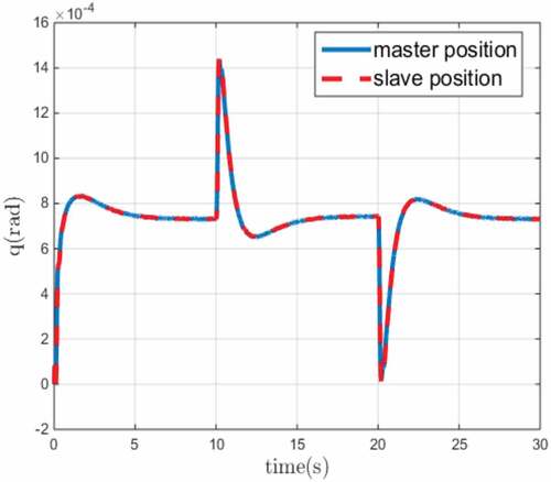
The exogenous force signals applied by the human operator in joint space are shown in Figure 1. The exogenous force signals are assumed to be square waves with amplitude 10N passing from the first order filter $\frac{1}{s+1}$. The position signals of the master and slave robot in joint space are also depicted in Figure 2 for the first joint and Figure 3 for the second joint. In both figures, the position of master and slave robots are depicted by solid blue line and dashed red line, respectively. The results demonstrate that the position of the slave robot tracks the position of the master robot with appropriate performance.

Figure 1. The force signals exerted by the human operator

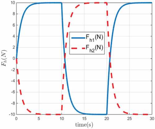
Figure 2. The position tracking for the first joint

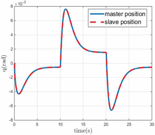
Figure 3. The position tracking for the second joint

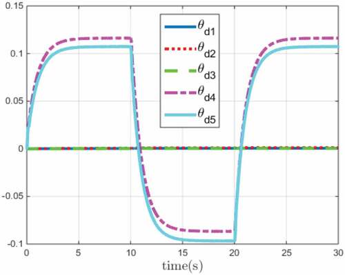
Furthermore, the estimation of the kinematic parameters and dynamic parameters of the master robot are shown in Figures 4 and 5, respectively. Since the parameter estimation of the slave robot have a similar behavior, the estimated dynamic and kinematic parameters are not shown to shorten the length of the article. As the results show, the estimated parameters have almost fixed values at steady state after short transitions. In fact, after each step change to the reference, the estimated parameters are affected accordingly. For instance, this issue is apparent at $t=10s$ in both Figures 4 and 5. Then, the estimated parameters reach to steady state after some transition. The estimated parameters remain in the steady state until the next change in the exogenous force at $t=20s$. Although the update lows fluctuate after any change on the exogenous force, the position tracking is always satisfactory. Such behavior is expected in any adaptive control system.

Figure 4. The convergence of the kinematic parameters for the master robot

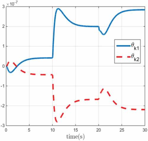
Figure 5. The convergence of the dynamic parameters for the master robot

6. Conclusions

This paper investigates the adaptive control design problem for teleoperation systems in the presence of time delay and uncertainty in both the dynamic and kinematic parameters. A control structure including control and adaptation laws are presented for the master and slave sides. The stability analysis of closed loop system is presented by considering the mentioned issues. Simulation results show the effectiveness of the proposed control structure. In the future studies, the effect of flexibility in the slave robot and multiple master robots can be considered. Another extension of the proposed approach is its combination with impedance control for implementation in sensitive applications such as telesurgery.

Additional information

Funding

The authors received no direct funding for this research.

Notes on contributors

Afshin Javid

The first author have received the M.Sc. degree from Islamic Azad University–South Tehran Branch, Tehran, Iran, while the second author is an associate professor there. Both authors are interested in developing advanced control methodologies with application in robotic systems. The authors conducted this research to solve the problems regarding kinematic uncertainty in the tele-robotic systems. This research is developed based on the previous investigation of the authors which was presented at an international conference.

References

- Abdeetedal, M., Rezaee, H., Talebi, H. A., & Abdollahi, F. (2018, Aug 31). Optimal adaptive Jacobian internal forces controller for multiple whole-limb manipulators in the presence of kinematic uncertainties. Mechatronics, 53, 1–18. doi:10.1016/j.mechatronics.2018.05.005
- Agand, P., Motaharifar, M., & Taghirad, H. D. (2017, October 1). Decentralized robust control for teleoperated needle insertion with uncertainty and communication delay. Mechatronics, 46, 46–59. doi:10.1016/j.mechatronics.2017.06.004
- Anderson, R. J., & Spong, M. W. (1989). Bilateral control of teleoperators with time delay. IEEE Transactions on Automatic Control, 34, 494–501. doi:10.1109/9.24201
- Cheah, C. C., Liu, C., & Slotine, J. J. (2006, March). Adaptive tracking control for robots with unknown kinematic and dynamic properties. The International Journal of Robotics Research, 25(3), 283–296. doi:10.1177/0278364906063830
- Chopra, N., Spong, M. W., & Lozano, R. (2008, August). Synchronization of bilateral teleoperators with time delay. Automatica, 44(8), 2142–2148. doi:10.1016/j.automatica.2007.12.002
- de Wit, C. C., Siciliano, B., & Bastin, G., editors. (2012, December). Theory of robot control. London: Springer Science & Business Media.
- Ferrell, W. R. (1966). Delayed force feedback. Human Factors: the Journal of the Human Factors and Ergonomics Society, 8, 449–455. doi:10.1177/001872086600800509
- Hashtrudi-Zaad, K., & Salcudean, S. E. (2002, February). Transparency in time-delayed systems and the effect of local force feedback for transparent teleoperation. IEEE Transactions on Robotics and Automation, 18(1), 108–114. doi:10.1109/70.988981
- Iqbal, J., Ullah, M. I., Khan, A. A., & Irfan, M. (2015, July). Towards sophisticated control of robotic manipulators: An experimental study on a pseudo-industrial arm. Strojniškivestnik-Journal of Mechanical Engineering, 61(7–8), 465–470. doi:10.5545/sv-jme.2015.2511
- Javid, A., & Ali Nekoui, M. (2018, October 23). An adaptive controller for bilateral teleoperation systems with uncertain kinematics and dynamics. In 2018 6th RSI International Conference on Robotics and Mechatronics (IcRoM) (pp. 59–64). Tehran: Iran University of Science & Technology.
- Lawrence, D. A. (1993, October). Stability and transparency in bilateral teleoperation. IEEE Transactions on Robotics and Automation, 9(5), 624–637. doi:10.1109/70.258054
- Liu, X., Tavakoli, M., & Huang, Q. (2010, October 18). Nonlinear adaptive bilateral control of teleoperation systems with uncertain dynamics and kinematics. InIntelligent Robots and Systems (IROS). 2010 IEEE/RSJ International Conference on (pp. 4244–4249). IEEE.
- Motaharifar, M., Talebi, H. A., Abdollahi, F., & Afshar, A. (2015, August). Nonlinear adaptive output-feedback controller design for guidance of flexible needles. IEEE/ASME Transactions on Mechatronics, 20(4), 1912–1919. doi:10.1109/TMECH.2014.2359181
- Nuño, E., Ortega, R., & Basañez, L. (2010, January). An adaptive controller for nonlinear teleoperators. Automatica, 46(1), 155–159. doi:10.1016/j.automatica.2009.10.026
- Polushin, I. G., Liu, X. P., & Lung, C. H. (2012, June). Stability of bilateral teleoperators with generalized projection-based force reflection algorithms. Automatica, 48(6), 1005–1016. doi:10.1016/j.automatica.2012.02.043
- Polushin, I. G., & Marquez, H. J. (2003, January). Stabilization of bilaterally controlled teleoperators with communication delay: An ISS approach. International Journal of Control, 76(8), 858–870. doi:10.1080/0020717031000116515
- Polushin, I. G., Tayebi, A., & Marquez, H. J. (2006, June). Control schemes for stable teleoperation with communication delay based on IOS small gain theorem. Automatica, 42(6), 905–915. doi:10.1016/j.automatica.2006.02.020
- Shahdi, A., & Sirouspour, S. (2009, February). Adaptive/robust control for time-delay teleoperation. IEEE Transactions on Robotics, 25(1), 196–205. doi:10.1109/TRO.2008.2010963
- Sharifi, I., Talebi, H. A., & Motaharifar, M. (2017, March). Robust output feedback controller design for time‐delayed teleoperation: Experimental results. Asian Journal of Control, 19(2), 625–635. doi:10.1002/asjc.1387
- Spong, M. W., Hutchinson, S., & Vidyasagar, M. (2006, December). Robot modeling and control. New York, NY: Wiley.