Numerical simulation of collision-free near-shortest path generation for Dubins vehicle via Hamilton–Jacobi–Bellman equation: A case study

Abstract

Motivated by modeling an unmanned aerial vehicle at a constant altitude plane above ground level as Dubins vehicle with signed upper-bounded curvature as constrained input and the flight path as Dubins path, the class of flight paths we study is restricted to the paths composed by path segments with zero or constant curvature satisfying the curvature constraint. We start with time-optimal control formulation incorporating mixed constraints for Dubins vehicle in cluttered planar environment and derive the associated Hamilton-Jacobi-Bellman (HJB) equation for the value function from the necessary time-optimality condition. The Kruzkov transform is used to modify the HJB equation for scaling of the solution to be bounded near the obstacles. Numerical solutions based on the fast-sweeping methods with consistent, monotone upwind Godunov Hamiltonian and semi-Lagrange methods are implemented for solving the two-point boundary value problem of modified HJB equation. Comparative validation simulations suggest the appropriateness of both schemes for the numerical collision-free shortest path via Kruzkov transformed HJB equation but with different convergence rate. Two schemes both perform satisfactory path planning, while Godunov Hamiltonian scheme provides more accurate in order of convergence. It is also found by example simulations that the grid resolution and time-step size required for switching structure is finer than that of the convergence criterion.

Keywords:

• Dubins path
• HJB equation
• Godunov Hamiltonian scheme
• semi-Lagrange scheme
• obstacle avoidance
• unmanned aerial vehicles

PUBLIC INTEREST STATEMENT

Unmanned aerial vehicles (UAVs) are emerging in commercial missions such as package delivery in cities, monitoring of typhoon or air quality PM 2.5. To achieve the mission goal, generation of flyable paths is crucial to the efficient operation of uavs with operating and vehicle constraints. Dubins vehicle is an ideal model for a UAV moving forward at constant speed at constant low altitude with curvature constraint. Dubins paths are the shortest path linking two configurations for a Dubins vehicle in the absence of obstacles. In the presence of obstacles such as radar sites and prohibited areas, Dubins path can be extended via numerical time- optimal control (bang-singular-bang) corresponding to the case of Dubins-like path composed by line and left or right turn of minimum turning radius. Assessment of accuracy of numerically obtained paths demonstrates the appropriateness of the numerical methods for path generation for given boundary conditions and obstacle distributions.

1. Introduction

State-to-state transfer is a common mobility task for bringing a system from an initial state to a target state. Among the many admissible state-to-state transfer trajectories in which the dynamics of the system is explicitly accounted for, the optimal maneuvering of unmanned vehicles that requires minimizing a cost functional, i.e., generation of constrained optimal input and state trajectories (or optimization-based physically realizable trajectory generation) or even better feedback motions, is challenging. In finding the input/control command that could be saturated on the convex compact set of constrained input, the optimal control formulations are powerful for optimal utilization of actuation capabilities. By following the standard optimal control formulation for the motion of a dynamic system described by state equations, it is possible that optimization of a multitude of cost functional (e.g. time-to-go, energy expenditure, distance or their mixture), especially for missions or tasks which are repeatedly executed a number of times by a dynamic system can be achieved. To solve for the state and control trajectories while optimizing a cost function subject to physical and environmental limitations described by the equality or inequality state and control constraints can be viewed as a type of model-based path planning or kinodynamic motion planning (Wolek & Woolsey, 2017). A wealth of numerical methods and tools has developed to optimize the control input and state trajectories, while their accuracies or efficiencies are validated across a variety of model systems and problems (Bardi & Capuzzo-Dolcetta, 2008; Consolini et al., 2019; Szuster & Hendzel, 2018; Tonon et al., 2017). For example, a tool FALCON.m (http://www.fsd.mw.tum.de/software/falcon-m/) for Matlab is developed to solve a wide variety of optimal control problems. PRONTO for trajectory optimization is another example (Aguiar et al., 2017).

A well- known optimal constrained trajectory that has been extensively studied is the time-optimal trajectory along which the optimizing bang-bang switching control command respecting the safe handling envelope drives the system from a start state to a goal state (belonging to a goal manifold) in minimum time. Time-optimal control and fastest possible motion generation have been employed for efficient operation of practical kinematic systems in the aerospace, mechatronics, vehicle and robotics applications, such as variable-stiffness-actuated (VSA) systems (Zhakatayev et al., 2017), double integrator (Castro & Koiller, 2013; Sundar & Shiller, 1997), the differential drive mobile robot (e.g. Poonawala & Spong, 2017; Manor et al., 2018), Dubins vehicle (Kaya, 2017; Takei & Tsai, 2013), car-like vehicle (Bertolazzi and Frego, 2018)- (Desaulniers, 1996), unmanned aerial vehicles (UAVs) (Consolini et al., 2019; Patten et al., 1994; Techy & Woolsey, 2009; Zollars et al., 2018), and aerospace systems (Zhu et al., 2017). The state-to-state transfer time depends on the aggressiveness of maneuver, given the input constraints, boundary conditions (in terms of position, velocity and acceleration). A computationally practical approach to time-optimal trajectory planning is the decoupled approach. Decoupled approach assumes that a geometric path is preplanned first for the system, so that time-optimal trajectory planning reduces to the generation of optimal velocity (a time scaling function) along the prespecified geometric path that meets the kinodynamic limits on the velocity and acceleration derived from the system dynamics are considered separately (see e.g. Bertolazzi and Frego, 2018; Jamhour & Andr’e, 1996; Zdesar & Škrjanc, 2018). Fast, accurate and robust numerical integration is developed for the decoupled approach to generate a time-optimal velocity profile by construction of the admissible region of safe speed for each vehicle position in the phase plane of distance-velocity (Pham, 2014). The decoupled approach is not fully dynamic optimization, since the shape and length of the path are not changed by the time-scaling function simultaneously (Zdesar & Škrjanc, 2018) during the optimization.

A general formulation of time-optimal state-to-state transfer trajectory planning in the cluttered environment and its numerical schemes can incorporate the mixed constraints, i.e., the path or safety constraints of obstacles with general shapes, not only input saturation constraint. It reduces to a two-point boundary value problem of a type of Hamilton–Jacobi–Bellman (HJB) partial differential equations (PDEs). HJB PDEs are derived from the first-order necessary conditions for the optimality of trajectory and control for a dynamic system based on Pontryagin Maximum Principle (PMP) or Dynamic Programming Principle (DPP). Central to numerically solve the HJB PDEs is the concept of viscosity solution defined by (Crandall & Lions, 1984), (Michael, 1983). They showed that any monotone (thus first order), finite difference methods (FDMs), consistent numerical Hamiltonian would yield the numerical solution of HJB equation, i.e. the value function (i.e. the value of the minimum cost), converge to the viscosity solution. Other numerical methods to approximate the value function (i.e. travel time or cost-to-go) solutions to the HJB PDEs associated with the time-optimal control problems, for example, pseudospectral method (orthogonal collocation method) where a proper choice of collocation points is crucial (Gong et al., 2009; Mehrali-Varjani et al., 2018), adaptive sparse grid method (Bokanowski et al., 2013), radial basis function (Ferretti et al., 2017) based on interpolation and collocation, continuation methods (Zhu et al., 2017), among others are also popular in numerical nonlinear optimal control, but they are beyond the scope of the paper. Very useful comparisons are provided among the performance of different numerical schemes for solving the HJB equations, usually limited to one or two dimensions due to curse of dimensionality (Falcone, 2013; Font & Pedregal, 2018; Mehrali-Varjani et al., 2018; Kang & Wilcox, 2017; Zhu et al., 2017). Falcone (2013) showed that the numerical solutions of HJB equation resulting from time-optimal control problems are feasible for systems with at most dimension 3 but can be raised up to 10 with a combination of policy iteration and value iteration schemes.

A constant speed UAV at constant low altitude above ground level is modeled as a Dubins vehicle (Chen et al., 2018; Lugo-Cárdenas et al., 2014; Techy & Woolsey, 2009; Tsourdos et al., 2010; Zollars et al., 2018). It is essential to determine a flyable, even aggressive path or trajectory for constrained UAV flight. Among the flyable paths, Dubins path is the shortest curvature-constrained path which connects the initial and final positions and matches heading directions at both ends in the plane in the absence of obstacles. First introduced in 1957 (Dubins, 1957), Dubins work on shortest bounded-curvature paths, now called Dubins path, is widely employed in generation of wheeled mobile robot trajectory and flyable level flight paths of UAVs (see e.g. Chen et al., 2018; Lugo-Cárdenas et al., 2014; Techy & Woolsey, 2009; Tsourdos et al., 2010; Wu et al., 2000; Yang & Kapila, 2002), Due to the nature of Dubins path that is composed by tangential circular arcs for meeting the boundary conditions and straight lines (see Section 2.2) in the absence of obstacles, we restrict the families of desired constrained flight paths in cluttered environment to Dubins-like paths, i.e. the class of flight paths that begins and ends with circular arcs with minimum turning radius suitable for serving as a near-optimal tangent-continuous reference generator for UAV flyable path at constant low altitude. The reformulation of Dubins path based on optimality principle as a time-optimal collision-free trajectory of Dubins vehicle (Castro & Koiller, 2013; Kaya, 2017; Takei & Tsai, 2013) is followed in this paper. A commonly adopted two-level sequential strategy for vehicle steering is first design a path at the higher level, then a path following control design at the lower level. By contrast, from the control design point of view, a great advantage of this reformulation is, that it naturally results in optimal state feedback control and state trajectory simultaneously for steering the vehicle, and provides the insights into the problem and solution structure. More importantly, it allows the consideration of path constraints resulting from obstacles that introduce additional significant difficulty, and thus extending the computation of shortest paths into more realistic and sophisticated situations (cluttered environments), not analytically solvable even for the simple double integrator (Sundar & Shiller, 1997). Instead of the HJB equation considered by (Takei & Tsai, 2013), we consider a slightly modified HJB equation via Kruzkov transform to avoid unboundedness in the initial condition (such as the region neighboring the obstacle) to assure the existence of viscosity solution and computational feasibility. The obtained approximate numerical value function that generates approximation to viscosity solution of HJB equation is used for numerical time-optimal path generation. For revealing the optimality of numerically obtained control and state trajectories of considered HJB equation of Dubins vehicle, the algorithms of our implementation choice to demonstrate are two historical numerical iterative algorithms, Godunov numerical Hamiltonian and semi-Lagrange scheme. The two algorithms are two typical methods satisfying the conditions of convergence (Tsai et al., 2017), which produce intermediate solutions ensuring a decrease in value function for every iteration, regardless of initial conditions, to converge to the final outcome. To implement those schemes, fast sweeping method is an efficient method that demonstrates impressive numerical results (Tsai et al., 2017; Zhao, 2005, 2016). The method is faster with complexity $O\left(N\right)$ and easier to implement than fast marching method whose complexity is $\mathrm{O}\left(\mathrm{N}\mathrm{l}\mathrm{o}\mathrm{g}\mathrm{N}\right)$, where $N$ is the number of grid points used in the computational domain. with fast sweeping method. As is well known, numerical methods based on discretization into grids will round the state (in particular, the vehicle heading) to elements of a fixed set of discretized states, and these roundoff errors can accumulate. The propagation of errors gives traversal time error, thus the optimality of the numerical schemes needs to be checked. The aim of this paper is to assess the optimality or accuracy of the collision-free paths obtained by the numerical implementations with comparison to analytical Dubins-like paths composed by two typical path primitives of line segments and circular arcs satisfying the curvature constraint and paths generated by Hybrid A*. A thorough investigation of the numerical issues of HJB equation for time-optimal trajectory generation of Dubins vehicle is beyond the scope of the paper.

The rest of the paper is organized as follows. Section 2 contains the introduction of Dubins path and time-optimal control reformulation of Dubins path along with the associated derivation of HJB equation summarized mainly from (Takei & Tsai, 2013). The modified HJB equation by Kruzkov transform is presented. The DPP is proven to be satisfied in the time-optimal problem and the value function is the unique viscosity solution of the equation. Section 3 presents two historical numerical methods for solving the modified HJB equation. In Section 4, feasibility study of numerical schemes is studied by verifying the solution accuracy or optimality via comparisons with the analytical Dubins path in a computational domain without obstacles and then extends to a computational domain with obstacles by comparisons with analytical Dubins-like paths and with the paths generated by Hybrid A*. In Section 5, we conclude the paper.

2. Generation of time-optimal trajectory for Dubins vehicle via HJB equation

Notations:

1. The workspace $\mathrm{\Omega }\subseteq R^2$is an open and connected set with any point $\mathbf{x}=\left(\mathrm{x},\mathrm{y}\right)\in \mathrm{\Omega }$.

2. ${\mathrm{\Omega }}_{free}=\mathrm{\Omega }\mathrm{\setminus }\cup \{P_k|k=1,\dots ,N\}$ is the free space in which the vehicle can move, where $\{P_k|k=1,\dots ,N\}$ are $\mathrm{N}$ obstacles in $\mathrm{\Omega }.$ Here, “\” denotes set difference operation.

3. The configuration space ${\mathrm{\Omega }}_{pose}={\mathrm{\Omega }}_{free}\times \left[0,2\pi \right]$ with any configuration denoted as $\mathbf{z}=\left(\mathrm{x},\mathrm{y},\theta \right)\in {\mathrm{\Omega }}_{pose.}$

4. $\left({\mathrm{x}}_{\mathrm{A}},{\mathrm{y}}_{\mathrm{A}},{\theta }_{\mathrm{A}}\right),\left({\mathrm{x}}_{\mathrm{B}},{\mathrm{y}}_{\mathrm{B}},{\theta }_{\mathrm{B}}\right)\in {\mathrm{\Omega }}_{pose}$ denote the given initial and final configurations, respectively.

5. T is the total time for travel or motion in ${\mathrm{\Omega }}_{pose}$ of the concerned Dubins vehicle.

6. The state trajectory at time $\mathrm{t}\in \left[0,T\right]$ of Dubins vehicle with current control $\alpha$ at $\mathrm{t}$ and initial condition $\left(\mathrm{x}\left(0\right),\mathrm{y}\left(0\right),\theta \left(0\right)\right)=\left({\mathrm{x}}_{\mathrm{A}},{\mathrm{y}}_{\mathrm{A}},{\theta }_{\mathrm{A}}\right)$ which is at $\mathrm{t}=0$ is denoted as $\left(\mathrm{x}\left(\mathrm{t}\right),\mathrm{y}\left(\mathrm{t}\right),\theta \left(\mathrm{t}\right)\right)\equiv z_{\left(x_A,y_A,{\theta }_A\right)}^{\alpha }\in {\mathrm{\Omega }}_{pose}$.

7. The set of admissible input

8. $\rho$ is minimum radius of left or right turning.

9. The minimum distance between a point $\mathbf{x}$ and the obstacle $P_k$ is denoted: $\mathrm{d}\mathrm{i}\mathrm{s}\mathrm{t}\left(\mathbf{x},\mathrm{\partial }{P}_k\right):=\underset{\mathbf{y}\in \mathrm{\partial }{P}_k}{inf}\mathrm{d}\mathrm{i}\mathrm{s}\mathrm{t}\left(\mathbf{x},\mathbf{y}\right)$, where$\mathrm{d}\mathrm{i}\mathrm{s}\mathrm{t}\left(\mathbf{x},\mathbf{y}\right)=\mathbf{x}-\mathbf{y}$ is the Euclidean distance between $\mathbf{x},\mathbf{y}\in \mathrm{\Omega }$.

10. $\mathrm{u}\left(\mathrm{x},\mathrm{y},\theta \right)$ denotes the value function, solution to HJB equation.

11. $\mathrm{\nabla }\mathrm{u}=\left({\mathrm{u}}_{\mathrm{x}},{\mathrm{u}}_{\mathrm{y}},{\mathrm{u}}_{\theta }\right)$ denotes the gradient of value function $\mathrm{u}\left(\mathrm{x},\mathrm{y},\theta \right)$.

12. ${\mathrm{t}}_{\mathrm{s}\mathrm{w}1},{\mathrm{t}}_{\mathrm{s}\mathrm{w}2}$ two switching times for CSC Dubins path.

2.1. Kinematics of Dubins vehicle

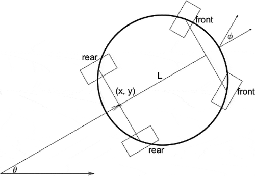
A Dubins vehicle platform (Figure 1) which is a very popular simplified four-wheeled model of high-fidelity vehicle with curvature constraint has been used as the unmanned ground, aerial or underwater vehicles. It attracts special interests in the study of UAV trajectory generation when the UAV fly only forward during a level flight with a constant altitude. In this paper, a Dubins vehicle is assumed a particle vehicle which can only move forward with constant speed $\mathrm{v}$ and with path maximal curvature bounded with.

Figure 1. A Dubins vehicle example considered in the paper.

With the arc length parametrization, the kinematics of a Dubins vehicle model with rolling and without slipping constraints is described as

(2.1) $\left\{\begin{array}{c}\frac{\mathrm{d}\mathrm{x}}{\mathrm{d}\mathrm{s}}=vcos\theta \left(s\right)\\ \frac{\mathrm{d}\mathrm{y}}{\mathrm{d}\mathrm{s}}=vsin\theta \left(\mathrm{s}\right)\\ \left|\frac{\mathrm{d}\theta }{\mathrm{d}\mathrm{s}}\right|\le \frac{1}{\rho }\end{array}\right.$(2.1)

where $\mathrm{s}$ is the arc-length along the path; $\left(\mathrm{x},\mathrm{y},\theta \right)\in {\mathrm{\Omega }}_{pose}$is the configuration of Dubins vehicle with tangent direction $\theta \left(\cdot \right)\in \left[0,2\pi \right)$ along the path, and it defines a unit tangent vector${\left[\mathrm{c}\mathrm{o}\mathrm{s}\theta ,\mathrm{s}\mathrm{i}\mathrm{n}\theta \right]}^{\mathrm{T}}$ along the path at the point $\mathrm{s}$; $\mathrm{v}$ is the constant speed of vehicle;

In Figure 1, $\rho =\frac{1}{{\kappa }_{max}}=\frac{{\omega }_{max}}{\mathrm{v}}$ is the minimal turning radius with ${\kappa }_{max}=\left(\mathrm{t}\mathrm{a}\mathrm{n}{\varphi }_{max}\right)/L$ and ${\omega }_{max}$ is maximal angular velocity (turn rate), where ${\varphi }_{max}$ is the maximum of steering angle $\varphi$ by front wheels and $L$ is the distance between the front and real axels of wheels.

The curvature is bounded due to bounded steering angle or minimum turn rate.

Now by changing the parameter $\mathrm{s}$ in (2.1) to time $\mathrm{t}>0$ via a time-scaling function $\mathrm{s}=\mathrm{s}\left(\mathrm{t}\right).$ Since $\frac{\mathrm{d}\theta }{\mathrm{d}\mathrm{t}}=\frac{\mathrm{d}\theta }{\mathrm{d}\mathrm{s}}\frac{\mathrm{d}\mathrm{s}}{\mathrm{d}\mathrm{t}}=\frac{\alpha \left(\mathrm{t}\right)}{\rho }\mathrm{v}$ with input $\alpha \left(\mathrm{t}\right)\in \left[-1,1\right]$, we obtain the following model:

(2.2) $\left\{\begin{array}{c}\frac{\mathrm{d}\mathrm{x}}{\mathrm{d}\mathrm{t}}=vcos\theta \left(\mathrm{t}\right)\\ \frac{\mathrm{d}\mathrm{y}}{\mathrm{d}\mathrm{t}}=vsin\theta \left(\mathrm{t}\right)\\ \frac{\mathrm{d}\theta }{\mathrm{d}\mathrm{t}}=\frac{\alpha \left(\mathrm{t}\right)}{\rho }v,\alpha \left(\mathrm{t}\right)\in \left[-1,1\right]\end{array}\right.$(2.2)

with a constraint on maximal angular velocity or equivalently maximal curvature (as $\alpha =\pm 1$),where + for left (counterclockwise, ccw) turn,—for right (clockwise, cw) turn. The signed curvature $\frac{\alpha \left(\mathrm{t}\right)}{\rho }$can be positive or negative that controls the rate of change of tangent direction (turn rate), for the motion of vehicle.

For more compactly, we denote:

(2.3) $\left(\begin{array}{c}\frac{\mathrm{d}\mathrm{x}}{\mathrm{d}\mathrm{t}}\\ \frac{\mathrm{d}\mathrm{y}}{\mathrm{d}\mathrm{t}}\\ \frac{\mathrm{d}\theta }{\mathrm{d}\mathrm{t}}\end{array}\right)=f\left(\mathrm{x},\mathrm{y},\theta ,\alpha \right):=\left[\begin{array}{c}\mathrm{v}\mathrm{c}\mathrm{o}\mathrm{s}\theta \\ \mathrm{v}\mathrm{s}\mathrm{i}\mathrm{n}\theta \\ \frac{\alpha }{\rho }\mathrm{v}\end{array}\right],\alpha \left(\mathrm{t}\right)\in \left[-1,1\right]$(2.3)

2.2. Brief on Dubins path and shortest path with obstacle-avoidance

The Dubins vehicle (2.2) has only three types of forward motion: straight, left turn and right turn with lowered bounded turning radius as the input.

The Dubins path is composed by concatenating circular arcs with maximum curvature and line segment tangential to circular arcs, so that at most three control input sequence of $\alpha \left(\mathrm{t}\right)=0,1,-1$ are sufficient to characterize the Dubins path.

This corresponds to, respectively, zero curvature (line) or constant speed forward translation, maximum curvature left(ccw) turn, maximum curvature right (cw) turn.

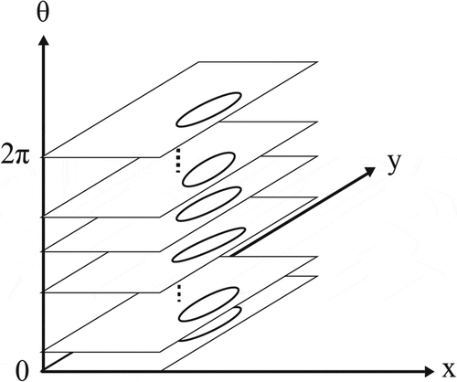
Figure 2. Discretization of configuration space as a finite set of slices. Each slice represents a two-dimensional subset of the discretized state space in the computational domain with heading of each node $\left(\mathrm{x},\mathrm{y}\right)$ in the slice chosen within the set of ${\mathrm{N}}_{\theta }$ discretized values over $\left[0,2\pi \right]$ (in the simulations, ${\mathrm{N}}_{\theta }=80$).

For given initial and final configurations, there are six types of shortest paths which is characterized in two families, namely CCC type and CSC type, where C denotes either the Left (L) or Right (R) turn circular arc of maximal curvature $\left(\frac{1}{\rho }\right)$, and S denote the straight line segment that is the common tangent line segment to the two circles tangential with the start and final poses. For the CSC type path (bang-singular-bang with two switching points) (Bui et al., 1994), the first turn is to turn from initial heading to the one end of line segment and the last turn is to turn from the other end of segment to the final heading. It is similar for the CCC type path (bang-bang type) except the middle one is a consecutive circular arc with beginning and end poses connecting to the end pose of first arc and the beginning of third arc, respectively. It is known that CSC has four possibilities: LSL and RSR, LSR and RS, while CCC has two possibilities: RLR and LRL of which the intermediate circular arc has an angle larger than $\rho \pi$ (Dubins, 1957). In general, CSC is more generic and common to occur than CCC for the distance pair of initial and final points is larger than $6\rho$ (Techy & Woolsey, 2009). So, for the case of state-to-state transfer with two end points far apart, the scenario in this paper’s (and others e.g. (Hota & Ghose, 2010; Pharpatara et al., 2015; Yang & Kapila, 2002) simulations, it takes the form of CSC (Kaya, 2017). It is clear that CSC type path is feasible for tangent-continuous constrained level flight path for UAVs.

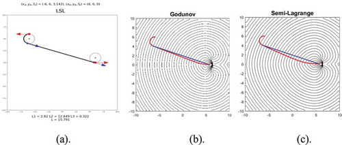
Figure 3. Example 2 (free environment). (a). The analytical CSC Dubins path. The length is about 15.79. (b). Level curves (black contours) and the path (red line) computed with Godunov Hamiltonian scheme. The length is 15.8162. The numerical value function $\mathrm{u}\left({\mathrm{x}}_A,{\mathrm{y}}_A,{\theta }_A\right)=15.9959$. (c) Level curves and the path computed with semi-Lagrange scheme. The length is 15.9784, slightly longer. The numerical value function $\mathrm{u}\left({\mathrm{x}}_A,{\mathrm{y}}_A,{\theta }_A\right)=16.0187$. For visualization, the tangential line segment to the entry and exit circles of (a) is $\mathrm{y}=-0.333\mathrm{x}+1.946$. It links from the first switching/tangential point (−6.3162, 4.0513) to another switching/tangential point (5.6838, 0.0513). The tangential line segment is superimposed onto the numerical trajectories of (b) and (c) (blue lines). The largest error in (b), (c) with respect to the optimal path is at the vincinity of the target.

However, though the tangent direction of Dubins path is continuous along the entire path, there are curvature (i.e. angular velocity) discontinuities in the junction of line and circular arc. Due to zero angular/rotational velocity and zero linear/translational velocity at two junctions of CSC path, there should be three acceleration-deceleration motion sequences along the first arc, straight line segment and the other arc of CSC path based on velocity limit curve generated from the state-dependent acceleration/input constraint and unicycle kinematics.

The work (Lugo-Cárdenas et al., 2014; Tsourdos et al., 2010; Yang & Kapila, 2002) aiming for application to UAV level flight path at low altitude provide a geometric construction of CSC type paths composed by four possible paths, the shortest of which is the Dubins path and is in closed form. It is also the way in the paper to determine the desired exact Dubins path with given initial and goal poses without obstacles. Note that the minimum radius turning circle of Dubins path for shortest path length could be relaxed to a range of admissible radii for UAV applications to offer flexibility in generation of Dubins-like paths (Chen et al., 2018). In (Manor et al., 2018; Wu et al., 2000), time-optimal velocity planning is studied for Dubins paths. Previous work (Castro & Koiller, 2013; Desaulniers, 1996; Liang et al., 2015; Sundar & Shiller, 1997;Yang et al.; Yang & Kapila, 2002) studied the length-shortest path which avoids obstacles.

(Liang et al., 2015) showed that length-minimal path should be composed of arc segments and line segments, and finding the shortest path which avoids obstacles is an NP hard problem. The works (Castro & Koiller, 2013; Desaulniers, 1996; Sundar & Shiller, 1997; Yang et al.; Yang & Kapila, 2002) (for only one circular obstacle) showed that the shortest path comprises of arc segments of maximum curvature, line segments and portion of the boundary of the obstacle.

2.3. Kruzkov transformed HJB equation for shortest path with obstacle-avoidance

Take advantage of the boundary-value problem of HJB equation resulting from Hamiltonian formulation to time-optimal trajectory generation problem was proposed and analyzed in (Castro & Koiller, 2013; Takei & Tsai, 2013; Sundar & Shiller, 1997). Because in the context, the speed $\mathrm{v}$ of Dubins vehicle (2.2) moving forward is constant, it is noted that the shortest path between two configurations is also time-optimal trajectory. The literature (Kaya, 2017; Takei & Tsai, 2013) reformulated the Dubins path (shortest curvature-constrained path in the plane) as the time-optimal trajectory generation of the control problem. In this approach, without obstacles, mathematically, the value function (the value of length-minimal Dubins path linking any initial pose to the given goal pose, as defined in (2.4)) is the solution to the HJB equation, whose ordinary differential equations for characteristic lines (in (2.12)) provides the necessary conditions of optimality of the control via PMP or DDP (see THEOREM 1) and state (position and heading) trajectory. The reformulation of characteristic line equations yields stationary solutions of bang-bang type (CCC type Dubins curve) where switching between $\alpha \left(\mathrm{t}\right)=1\mathrm{a}\mathrm{n}\mathrm{d}\alpha \left(\mathrm{t}\right)=-1$ may occur, or a concatenation of bang and singular arcs as bang-singular-bang type (CSC type Dubins curve) where at most two switchings between $\alpha \left(\mathrm{t}\right)=1,\alpha \left(\mathrm{t}\right)=0$ and between $\alpha \left(\mathrm{t}\right)=0,\alpha \left(\mathrm{t}\right)=-1$ may occur (Bui et al., 1994). Therefore, this allows the extension of Dubins path to the computation of shortest path or time-optimal trajectory of Dubins vehicle in cluttered environment (Takei & Tsai, 2013), where the obstacles are represented by environment or path constraints imposed on the motion of (2.2), and in 3D environment (Hota & Ghose, 2010; Pharpatara et al., 2015), or incorporation the effect of wind into the UAV flight (Techy & Woolsey, 2009).

We start the reformulation of HJB equation via PMP or DDP from the constrained optimal control problem whose cost is identity during the travel time which is required for the Dubins vehicle to move from the initial configuration to the goal configuration with the following constraints.

• (i) The vehicle model (2.2) with constant speed .

• (ii) The set of admissible control ${\mathbf{A}}_{\mathrm{a}\mathrm{d}}$ due to actuator saturation (equivalent to define the maximum angular velocity or maximum curvature of Dubins vehicle) is compact, convex.

• (iii) Safety/obstacle avoidance/state constraints on account of obstacles or forbidden zones: Let the signed distance field

${\mathrm{\Psi }}_k\left(\mathbf{x}\right)=\left\{\begin{array}{c}dist\left(\mathbf{x},\mathrm{\partial }{P}_k\right),ifx\notin P_k\\ -dist\left(\mathbf{x},\mathrm{\Omega }\mathrm{\setminus }\mathrm{\partial }{P}_k\right),ifx\in P_k\end{array}\right.$ for $\mathrm{k}=1,2,\dots ,\mathrm{N}$.

be positive, since ${\varphi }_k\left(\mathbf{x}\right)\le 0$ if and only if $\mathbf{x}\in P_k$.

The state constraints enforced by the obstacles to be avoided define the feasible region by ${\mathrm{\Psi }}_k\left(\mathbf{x}\left(\mathrm{t}\right)\right)\le$0, $\mathrm{t}\in \left[0,T\right].$For circular obstacle, the collision condition simplified to a safety zone represented by a circular constraint function $\mathbf{x}-r_k\le d_s$, where $d_s$ is a user-defined safety distance to account for the size of the vehicle, so that the robot could be reasonably shrunk into a point.

• (i) The boundary conditions are given: ${\mathbf{z}}_A=\left({\mathrm{x}}_{\mathrm{A}},{\mathrm{y}}_{\mathrm{A}},{\theta }_{\mathrm{A}}\right)$is the initial pose where the constant speed Dubins vehicle starting from $\left({\mathrm{x}}_{\mathrm{A}},{\mathrm{y}}_{\mathrm{A}}\right)\in {\mathrm{\Omega }}_{free}$; ${\mathbf{z}}_{\mathrm{B}}=\left({\mathrm{x}}_{\mathrm{B}},{\mathrm{y}}_{\mathrm{B}},{\theta }_{\mathrm{B}}\right)$ is the final pose where the vehicle reaches the goal $\left({\mathrm{x}}_{\mathrm{B}},{\mathrm{y}}_{\mathrm{B}}\right)\in {\mathrm{\Omega }}_{free}$. The final pose could be relaxed to be a compact region $\mathrm{\Sigma }$ for different simulation purposes.

Now, the value function (or so called cost-to-go function in control theory) of the problem can be so defined the minimum time cost of the path from an initial state $\left(\mathrm{x},\mathrm{y},\theta \right)$ to the state$\left({\mathrm{x}}_{\mathrm{B}},{\mathrm{y}}_{\mathrm{B}},{\theta }_{\mathrm{B}}\right)$ (or $\left\{\left({\mathrm{x}}_{\mathrm{B}},{\mathrm{y}}_{\mathrm{B}},{\theta }_{\mathrm{B}}\right)\in \mathrm{\Sigma }\right\}$):

(2.4) $\mathrm{u}\left(\mathrm{x},\mathrm{y},\theta \right)=\mathrm{i}\mathrm{n}\mathrm{f}\left\{T\ge 0:\alpha \in {\mathbf{A}}_{\mathbf{a}\mathbf{d}}\right\}$(2.4)

Since$\alpha \in {\mathbf{A}}_{\mathbf{a}\mathbf{d}}$is with all aforementioned constraints satisfied, the definition is both valid with or without obstacles. If there is no feasible path ${\mathbf{z}}_{\left(\mathrm{x},\mathrm{y},\theta \right)}^{\alpha \left(\cdot \right)}$ then we take the convention $\mathrm{u}\left(\mathrm{x},\mathrm{y},\theta \right)=\mathrm{\infty }$.

Remark. Only convex state constraints resulting from nonlinear inequality constraints representing obstacle avoidance are considered, more complex nonconvex state constraints require additional transformation or convexification. In this formulation, obstacles are hard constraints so that the trajectory is dynamically feasible and is guaranteed to be collision-free, in addition to time-optimal. Therefore, for guaranteed obstacle avoidance, obstacle is better represented as state constraint as above, instead of augmenting into the cost function.

The following restates essential principles and theorems used for derivation of the HJB equation for the Dubins vehicle (2.2) from the value function (2.4) using variational arguments.

THEOREM 1 (Bardi & Capuzzo-Dolcetta, 2008; Tonon et al., 2017): If the initial pose $\left(\mathrm{x},\mathrm{y},\theta \right)$ is given, $u\left(\mathrm{x},\mathrm{y},\theta \right)$ is defined by (2.4), then it satisfies the DPP (where the time step$\tau$ is so small such that $0<\tau <\mathrm{u}\left(\mathrm{x},\mathrm{y},\theta \right)$):

(2.5) $\mathrm{u}\left(\mathrm{x},\mathrm{y},\theta \right)=inf\left\{\tau +\mathrm{u}\left(\mathrm{x}\left(\tau \right),\mathrm{y}\left(\tau \right),\theta \left(\tau \right)\right):\mathrm{o}\mathrm{v}\mathrm{e}\mathrm{r}\mathrm{a}\mathrm{l}\mathrm{l}{\mathbf{z}}_{\left(x,y,\theta \right)}^{\alpha \left(\cdot \right)},\alpha \in {\mathbf{A}}_{\mathrm{a}\mathrm{d}}\right\}$(2.5)

Now applying Taylor expansion to $\mathrm{u}$ in (2.5), dividing by $\tau$ and let $\tau \to 0$, we transform (2.5) to obtain the follwoing:

Applying (2.2) to , since all possibly desired paths must satisfy (2.2) under any $\alpha \in {\mathbf{A}}_{\mathrm{a}\mathrm{d}}$, the above equation yields

(2.6) $-1=\underset{\alpha \left(\cdot \right)\in {\mathbf{A}}_{\mathrm{a}\mathrm{d}}}{\mathrm{i}\mathrm{n}\mathrm{f}}\left\{\mathrm{v}\mathrm{c}\mathrm{o}\mathrm{s}\theta {\mathrm{u}}_{\mathrm{x}}+\mathrm{v}\mathrm{s}\mathrm{i}\mathrm{n}\theta {\mathrm{u}}_{\mathrm{y}}+\frac{\alpha \left(\mathrm{t}\right){\mathrm{u}}_{\theta }}{\rho }\mathrm{v}\right\}$(2.6)

This concludes the optimal state feedback control, i.e. the optimal mapping from the optimal state trajectory to the optimal control trajectory, is determined by the sign of ${\mathrm{u}}_{\theta }$ which coincides the bang-bang principle that only one actuator is saturated (reaches the border of the input constrained set) at a time

(2.7) ${\alpha }^{\ast }\left(\mathrm{x},\mathrm{y},\theta \right)=-sgn\left({\mathrm{u}}_{\theta }\right)\in \left\{0,\pm 1\right\}$(2.7)

(2.7) coincides the bang-bang principle that only one actuator is saturated (reaches the border of the input constrained set) at a time. Thus, (2.6) leads to the HJB equation as introduced in (Takei & Tsai, 2013) which the value function $\mathrm{u}$ satisfies:

(2.8) $-\mathrm{v}cos\left(\theta \right){\mathrm{u}}_{\mathrm{x}}-\mathrm{v}\mathrm{s}\mathrm{i}\mathrm{n}\left(\theta \right){\mathrm{u}}_{\mathrm{y}}+\frac{\left|{\mathrm{u}}_{\theta }\right|}{\rho }\mathrm{v}-1=0$(2.8)

which has the boundary conditions:

(2.9) $\mathrm{u}\left(\mathrm{x},\mathrm{y},\theta \right)=0,\mathrm{i}\mathrm{f}\left(\mathrm{x},\mathrm{y},\theta \right)\in \mathrm{\Sigma }$(2.9)

(2.10) $\mathrm{u}\left(\mathrm{x},\mathrm{y},\theta \right)=\mathrm{\infty },\mathrm{i}\mathrm{f}\left(\mathrm{x},\mathrm{y},\theta \right)\in {\cup }_i{P}_i\times \left[0,2\pi \right]$(2.10)

(2.11) $\mathrm{u}\left(\mathrm{x},\mathrm{y},2\pi \right)=\mathrm{u}\left(\mathrm{x},\mathrm{y},0\right),if\left(x,y\right)\in {\mathrm{\Omega }}_{free}$(2.11)

where, (2.9) is trivial from the definition of (2.4), The infinite boundary condition (2.10) describes when the vehicle collides with obstacles, it will never go any further to the final pose. (2.11) is the periodic boundary condition because $\left(\mathrm{x},\mathrm{y},0\right)$, $\left(\mathrm{x},\mathrm{y},2\pi \right)$ denote the same pose of the vehicle.

Since for linear/nonlinear first-order PDE, there is also a resolution method called the method of characteristics. As the PDE is (2.8), the equations of characteristic lines are:

(2.12) $\left\{\begin{array}{c}\frac{\mathrm{d}\mathrm{x}}{\mathrm{d}\mathrm{t}}=vcos\theta \\ \frac{\mathrm{d}\mathrm{y}}{\mathrm{d}\mathrm{t}}=vsin\theta \\ \frac{\mathrm{d}\theta }{\mathrm{d}\mathrm{t}}=-\frac{\mathrm{s}\mathrm{i}\mathrm{g}\mathrm{n}\left({\mathrm{u}}_{\theta }\right)}{\rho }v=\frac{{\alpha }^{\ast }\mathrm{v}}{\rho }\end{array}\right.\mathrm{w}\mathrm{i}\mathrm{t}\mathrm{h}\mathrm{i}\mathrm{n}\mathrm{i}\mathrm{t}\mathrm{i}\mathrm{a}\mathrm{l}\mathrm{c}\mathrm{o}\mathrm{n}\mathrm{d}\mathrm{i}\mathrm{t}\mathrm{i}\mathrm{o}\mathrm{n}\mathrm{s}\left(\begin{array}{c}x\left(0\right)\\ y\left(0\right)\\ \theta \left(0\right)\end{array}\right)=\left(\begin{array}{c}{\mathrm{x}}_{\mathrm{A}}\\ {\mathrm{y}}_{\mathrm{A}}\\ {\theta }_{\mathrm{A}}\end{array}\right)$(2.12)

Remarks. (i) Since (2.7), the optimal control at any $\mathrm{t}>0$ coincides to the bang-bang principle, it is necessary to make assumption that the obstacle boundaries have curvature larger than $\frac{1}{\rho }$.

(ii) HJB equation (2.8)(2.8) $-\mathrm{v}cos\left(\theta \right){\mathrm{u}}_{\mathrm{x}}-\mathrm{v}\mathrm{s}\mathrm{i}\mathrm{n}\left(\theta \right){\mathrm{u}}_{\mathrm{y}}+\frac{\left|{\mathrm{u}}_{\theta }\right|}{\rho }\mathrm{v}-1=0$(2.8) derived from value function (2.4) also leads to the result that Hamiltonian is zero along the time-optimal trajectories of Dubins vehicle (2.2) for free terminal time (Szuster & Hendzel, 2018) and zero terminal cost (Mehrali-Varjani et al., 2018).

(iii) For any starting pose $\left(\mathrm{x},\mathrm{y},\theta \right)$ such that $\mathrm{u}\left(\mathrm{x},\mathrm{y},\theta \right)$ is finite, there is an optimal control ${\alpha }^{\ast }\in {\mathbf{A}}_{\mathrm{a}\mathrm{d}}$ which navigates the vehicle from $\left(\mathrm{x},\mathrm{y},\theta \right)$ to $\left({\mathrm{x}}_{\mathrm{B}},{\mathrm{y}}_{\mathrm{B}},{\theta }_{\mathrm{B}}\right)\in \mathrm{\Sigma }$. From THEOREM 1, the value function decreases as the vehicle follows ${\alpha }^{\ast }$. Therefore, $\mathrm{u}\left(\mathrm{x},\mathrm{y},\theta \right)$ could not be a local minimum of the value function if $\mathrm{u}\left(\mathrm{x},\mathrm{y},\theta \right)$ is only finite.

(iv) A practical advantage of the optimal control in state feedback form (2.7) resulting naturally from the value function solution of the HJB equation (Guo & Wu, 2017) is robust with respect to computation and modeling errors (Mehrali-Varjani et al., 2018). Only the gradient of optimal value function (or the optimal value function over a small neighborhood) of the current state, is required for constructing time-optimal state feedback control (2.7). In addition, the HJB equation approach allows the construction of whole characteristic lines (2.12) for finding a time-optimal trajectories between any given pair of initial and final configurations in the free configuration space, while analytical or geometric construction based on Dubins path is feasible only for one specific pair of initial-final configurations and has the advantage of constant computation time, independent of the spatial and temporal resolutions or the number of grids and time step size.

However, on the region where either the obstacles occupy or no feasible path exists, the value function is infinite that causes ill numerical issues. To tackle with it, let’s introduce the Kruzkov transform (Falcone, 2013; Tonon et al., 2017):

(2.13) $w=\left\{\begin{array}{c}1-{\mathrm{e}}^{-u},u<\mathrm{\infty }\\ 1,u=\mathrm{\infty }\end{array}\right.$(2.13)

So THEOREM 1 (or the DPP (Bardi & Capuzzo-Dolcetta, 2008)) should be rewritten for the corresponding new value function:

(2.14) $w\left(\mathrm{x},\mathrm{y},\theta \right)=inf\left\{1-e^{-\tau }+e^{-\tau }w\left(\mathrm{x}\left(\tau \right),\mathrm{y}\left(\tau \right),\theta \left(\tau \right)\right):\mathrm{o}\mathrm{v}\mathrm{e}\mathrm{r}\mathrm{a}\mathrm{l}\mathrm{l}{\mathbf{z}}_{\left(\mathrm{x},\mathrm{y},\theta \right)}^{\alpha \left(\cdot \right)}\mathrm{w}\mathrm{i}\mathrm{t}\mathrm{h}\alpha \left(\cdot \right)\in {\mathbf{A}}_{\mathrm{a}\mathrm{d}}\right\}$(2.14)

With this transform, we could derive again via above process the following transformed PDE:

(2.15) $w-\mathrm{v}cos\left(\theta \right)w_{\mathrm{x}}-\mathrm{v}\mathrm{s}\mathrm{i}\mathrm{n}\left(\theta \right)w_{\mathrm{y}}+\frac{\mathrm{v}}{\rho }\left|w_{\theta }\right|-1=0$(2.15)

which satisfies the corresponding boundary conditions:

(2.16) $\left\{\begin{array}{c}w\left(\mathrm{x},\mathrm{y},\theta \right)=0,if\left(\mathrm{x},\mathrm{y},\theta \right)\in \mathrm{\Sigma }\\ w\left(\mathrm{x},\mathrm{y},\theta \right)=1,if{\mathrm{\Psi }}_k\left(\mathrm{x},\mathrm{y}\right)>0,\theta \in \left[0,2\pi \right]forallk\\ w\left(\mathrm{x},\mathrm{y},2\pi \right)=w\left(\mathrm{x},\mathrm{y},0\right),if{\mathrm{\Psi }}_k\left(\mathrm{x},\mathrm{y}\right)>0forallk\end{array}\right.$(2.16)

For simplicity, we write $\mathrm{H}=\mathrm{H}\left(\mathrm{D}w\right):=-\mathrm{v}cos\left(\theta \right)w_{\mathrm{x}}-\mathrm{v}\mathrm{s}\mathrm{i}\mathrm{n}\left(\theta \right)w_{\mathrm{y}}+\frac{\mathrm{v}}{\rho }\left|w_{\theta }\right|-1$ unless an ambiguity occurs.

Now, the Kruzkov transformed value function (2.13) which is well-defined by (2.4) is the solution of (2.15) with boundary conditions (2.16). But what kind of solution is it? It is known that the Dubins vehicle does not satisfy the small-time locally controllable condition (or STLC condition) introduced in (Bardi & Capuzzo-Dolcetta, 2008; Takei & Tsai, 2013). That is equivalent to say $\mathrm{w}$ is discontinuous on a neighborhood of $\left({\mathrm{x}}_{\mathrm{B}},{\mathrm{y}}_{\mathrm{B}},{\theta }_{\mathrm{B}}\right)\in \mathrm{\Sigma }$. Mathematically, there is not always the classical smooth solution for a general HJB equation with initial/boundary conditions. Therefore, several concepts of solutions (like, weak solutions, generalized solutions, viscosity solutions … etc.) are raised to overcome this drawback. In these solutions, the viscosity solution is well accepted as a reasonable solution. The “reasonable” means it may occur (or appear) in the real physical world. Another advantage of taking it as solution is it shares many good properties, including, existence theorem (by the method of vanishing viscosity or Perron’s method), uniqueness theorem and stability (The uniform limit of solutions is a viscosity solution). However, in this case, we do not require the viscosity solution to be necessarily bounded and uniformly continuous. It belongs to a more general kind of solution called discontinuous viscosity solution, introduced in (Bardi & Capuzzo-Dolcetta, 2008; Takei & Tsai, 2013). In most cases, numerical schemes are required to solve the value function, or the time-optimal collision-free trajectory generation of Dubins vehicle (2.2). We should mention that there is a wealth of literature on numerical solutions of HJB equations. It is desirable to know which numerical schemes for which problem give the correct interpretation of results. The main goal of the case study of Dubins paths in this paper is to reveal the numerical issues related to accurate time-optimal trajectory computation for Dubins vehicle through the application of two numerical schemes for the considered HJB equation.

Remarks. (i) In the case of constant speed, (2.2) is differentiated to obtain

$\frac{{\mathrm{d}}^2}{\mathrm{d}{\mathrm{t}}^2}\left(\begin{array}{c}x\\ y\\ \theta \end{array}\right)=\left[\begin{array}{c}-sin\theta \\ cos\theta \\ 0\end{array}\right]\frac{\alpha \left(\mathrm{t}\right)}{\rho }{\mathrm{v}}^2,\alpha \left(\mathrm{t}\right)\in \left[-1,1\right]$

for a path composed of straight line and circular arcs so that $\frac{\mathrm{d}\alpha }{\mathrm{d}\mathrm{t}}=0.$The term $\frac{\alpha \left(\mathrm{t}\right)}{\rho }{\mathrm{v}}^2$ is the normal acceleration of the vehicle orthogonal to velocity, while the tangential acceleration is always zero for following a Dubins-like path composed of straight line segments and tangential circular arcs.

(ii) Depending on the level of complexity and accuracy of models required, the modeling issues such as incorporation of other quantities as state or control variables are related to model-based time-optimal trajectory and control. Differential drive mobile robot is a typical Dubins vehicle. It can be modeled as torque-controlled system, and when the vehicle is driven as fast as possible, its bang-bang control (input torque profile is at its limit) was solved by PMP (Poonawala & Spong, 2017). An extended acceleration-controlled Dubins vehicle model of (2.2) is to use instead of variable speed v (Ben-Asher et al., 2020; Wolek et al., 2016), the constrained tangential acceleration ${\alpha }_1=\frac{\mathrm{d}\mathrm{v}}{\mathrm{d}\mathrm{t}},\hspace{0.17em}{\alpha }_1\le {\alpha }_{1\mathrm{b}}$ as one input, in addition to the angular velocity input ${\alpha }_2=$ $\frac{\alpha \left(\mathrm{t}\right)}{\rho }\mathrm{v}$ (or equivalently the lateral/normal acceleration$\frac{\alpha \left(\mathrm{t}\right)}{\rho }{\mathrm{v}}^2$) that is orthogonal to the path tangent/velocity vector (Manor et al., 2018) as Dubins vehicle (2.2). The inclusion of non-zero tangential acceleration in vehicle model complicates the time-optimal solution. In (Manor et al., 2018), the solution to time-optimal trajectory of extended Dubins vehicle model involves the simple quadrature, and the gradient is computed by IPOPT or FALCON.m. Another aspect regarding the model is that he bound of admissible control/curvature in (2.2) is assumed symmetric so that both right and left turn are allowed, as well as zero input that yields straight line motion. The work (Fedotov & Patsko, 2018) considers the general bound on the admissible control, which can be asymmetric and not include zero input. Another work (Zollars et al., 2018) considers the use of angular acceleration (second derivative of heading) as the control input to Dubins vehicle.

3. Two numerical schemes

HJB equations are a general type of PDEs which comes from many different fields, like optimal control and trajectory optimization of mechatronic systems studied in this paper, differential games (Botkin et al., 2011), geometrical optics and computer vision. Eikonal equation is one well-known example of HJB equations that motivates the FSM and other numerical techniques. This section introduces the methods of our numerical implementation for two-point boundary value problem resulting from the necessary time-optimality condition.

3.1. Brief on numerical methods for HJB PDE

A HJB PDE can be solved numerically in different ways. It is well understood that there is no general numerical method for all kinds of HJB equations in terms of accuracy and efficiency. FDM and finite element method (FEM) are two dominant numerical methods for solving PDEs. The former is via direct discretization called finite differences for approximating gradient of value function and the latter uses a linear combination of basic functions such as polynomials or trigonometric polynomials to approximate solutions of variational formulations. Because the HJB equations and hyperbolic PDEs of conservation laws have many mathematical similarities in common, advances in the conceptual principles and higher-order methods for conservation laws are borrowed as effective solvers for the HJB equations (Kao et al., 2004; Tsai et al., 2017; Zhao, 2005, 2016). Firstly, Crandall and Lions (1984) and Michael (1983) first proposed not only an adequate weak solution for HJB equations, namely, viscosity solution, but also along with a principle that any monotone, differenced form with consistent numerical Hamiltonian must converges to its viscosity solution (Crandall & Lions, 1984). Now it is well understood that the convex HJB equation can be solved with monotone upwind scheme on general meshes, such as discussed in (Wang et al., 2000).

For a time-independent HJB equation, as the discretization of HJB equation (2.15)(2.15) $w-\mathrm{v}cos\left(\theta \right)w_{\mathrm{x}}-\mathrm{v}\mathrm{s}\mathrm{i}\mathrm{n}\left(\theta \right)w_{\mathrm{y}}+\frac{\mathrm{v}}{\rho }\left|w_{\theta }\right|-1=0$(2.15) is determined, a suitable iteration method is needed because the equation is lack of time-evolution. The FSM is a well-known iteration method which is firstly invented in (Zhao, 2005). It is a powerful and effective method for computing first-order linear or nonlinear PDE solution due to two reasons: (i) it matches the corresponding upwind direction that allows information along characteristics efficiently; and (ii) it is an iterative method which applies the Gauss-Seidel method to accelerate convergence based on the idea of alternating the order that the grid nodes are visited with different directions in which characteristic lines might be along (Zhao, 2005, 2016). To (i), it can be shown that a consistent upwind scheme is a monotone differenced form and therefore, it converges to the viscosity solution with at most first-order accurate (Crandall & Lions, 1984). The Hamiltonian in Godunov scheme from solving conservation laws is one example of such schemes. For solving stationary HJB equation, FSM iteratively evaluates the values upwind (i.e. propagates the information upward to a neighboring grid with subsequent path cost decreased) or along characteristic lines for updating the solution. FSM is faster with complexity O (N) and easier to implement than FMM which is with complexity (NlogN) (where N is the number of grid points used in the grid system) (Zhao, 2005, 2016). To the other key ingredient, the motivation behind it is the information of solution of the HJB equation propagates along characteristics. All characteristics can be divided into a finite number of pieces according to their directions and each one can be covered by one of the sweeping orderings simultaneously. The number of iterations is proportional to the maximum number of pieces for all characteristics. Moreover, values at all grid points are monotonically non-increasing with iterations. Once the correct value at a grid point is obtained it will not be changed in later iterations (Zhao, 2016).

3.2. Solving numerical schemes by fast sweeping method (FSM)

Though both time-optimal control and state trajectories can be obtained by numerical methods of solving Kruzkov modified HJB equation, implementation issues encountered are: (i) The numerical solvers are iterative in nature, where the update direction and the step size of each iteration need to be computed. (ii) In addition, choice of initial guess and avoiding stuck in local minima such as saddle trajectories are required for fast and accurate convergent solution. A choice of an appropriate numerical scheme is essential to obtain a satisfying solution for the specific problem considered here with a compromise between accuracy (time step for numerical integration and state grid resolution) and speed or real-time feasibility (computation time). The choice should be on the basis of implementing numerical solvers, possibly combined with the knowledge of the problem or the system. In this section, among a large class of numerical methods available for solving the value function of the discrete finite-time HJB equation, we use the fast-sweeping method (FSM) (Takei & Tsai, 2013; Tsai et al., 2017; Zhao, 2005, 2016). For FSM, ordering of grid nodes is based on causality principle. Two historical numerical schemes, numerical Hamiltonian in Godunov scheme and semi-Lagrange method, are introduced here, where (2.14) is the foundation of semi-Lagrange scheme (Bardi & Capuzzo-Dolcetta, 2008; Takei & Tsai, 2013) and (2.15) is the foundation of Godunov scheme. One reason for the choice of the methods to use is both methods are based on FDM, which is robust and easy to implement. The other is accuracy of first-order methods suffices for presenting time-optimal, collision-avoidance trajectory generation via HJB equation approach. The optimality (approximation error) of the paths obtained using various numerical algorithms is controlled by the grid resolution and time discretization, which are shown later in simulations.

3.3. Discretization of Kruzkov transformed HJB

3.3.1. Godunov scheme

We first discretize the transformed HJB Equation (2.15)(2.15) $w-\mathrm{v}cos\left(\theta \right)w_{\mathrm{x}}-\mathrm{v}\mathrm{s}\mathrm{i}\mathrm{n}\left(\theta \right)w_{\mathrm{y}}+\frac{\mathrm{v}}{\rho }\left|w_{\theta }\right|-1=0$(2.15) in state space. By spatial discretization of the computational domain of configuration space ${\mathrm{\Omega }}_{pose}$ (as depicted in Figure 2) into ${\mathrm{N}}_x\times {\mathrm{N}}_y\times {\mathrm{N}}_{\theta }$ grid points with grid size $h_x,h_y$, respectively, in x-,y- variables which corresponds to the discrete $\theta$ - variable with grid size $h_{\theta }$ in [0, $2\pi$]. Let the notation

${\mathrm{W}}_{ijk}:=\mathrm{w}\left(x_i,y_j,{\theta }_k\right)$

be the approximation value function of $\mathrm{w}$ at the grid point $\left(x_i,y_j,{\theta }_k\right)$.

The derivatives of $\mathrm{w}$ with respect to the arguments are then approximated by the corresponding finite difference expressions. Thus, the approximated sided- differences with respect to $\mathrm{x}$ is defined:

${\mathrm{\Delta }}_x^{-}{W}_{ijk}=\frac{W_{i,j,k}-W_{i-1jk}}{h_x}$

${\mathrm{\Delta }}_x^{+}{W}_{ijk}=\frac{W_{i+1,j,k}-W_{ijk}}{h_x}$

for ${\mathrm{w}}_x$. Similar notations could be defined to approximate the derivatives ${\mathrm{w}}_y$ and ${\mathrm{w}}_{\theta }$. Finally, as mentioned above, a suitable numerical Hamiltonian make the numerical solution converges to the desired viscosity solution. A numerical Hamiltonian $\hat{\mathrm{H}}\left(a^{-},a^{+},b^{-},b^{+},c^{-},c^{+}\right)$ with six variables needs to be monotone, if $\hat{\mathrm{H}}\left(\uparrow ,\downarrow ,\uparrow ,\downarrow ,\uparrow ,\downarrow \right)$ holds, where $\uparrow ,\downarrow$means $\hat{\mathrm{H}}$ monotonically non-decreasing, non-increasing in the variables, respectively; and consistent, if $\hat{\mathrm{H}}\left(u,u;v,v;w,w\right)=\mathrm{H}\left(u,v,w\right)$ holds.

Thus a consistent, monotone and Lipschitz continuous of all variables numerical Hamiltonian $\hat{\mathrm{H}}$ for the HJB Equation (2.15)(2.15) $w-\mathrm{v}cos\left(\theta \right)w_{\mathrm{x}}-\mathrm{v}\mathrm{s}\mathrm{i}\mathrm{n}\left(\theta \right)w_{\mathrm{y}}+\frac{\mathrm{v}}{\rho }\left|w_{\theta }\right|-1=0$(2.15) leads to the following form:

$W_{ijk}+\hat{\mathrm{H}}\left({\mathrm{\Delta }}_x^{-}{W}_{ijk},{\mathrm{\Delta }}_x^{+}{W}_{ijk};{\mathrm{\Delta }}_y^{-}{W}_{ijk},{\mathrm{\Delta }}_y^{+}{W}_{ijk};{\mathrm{\Delta }}_{\theta }^{-}{W}_{ijk},{\mathrm{\Delta }}_{\theta }^{+}{W}_{ijk}\right)=0$

As being introduced in (Kao et al., 2004; Tsai et al., 2017; Zhao, 2005), the Godunov Hamiltonian scheme for a nonnegative, Lipschitz continuous and strictly convex Hamiltonian (which (3.15) satisfies) is provided as the following:

(3.1) $H^G\left(p^{-},p^{+},q^{-},q^{+},r^{-},r^{+}\right)=\underset{p\in I\left[p^{-},p^{+}\right]}{\mathrm{e}\mathrm{x}\mathrm{t}}\underset{q\in I\left[q^{-},q^{+}\right]}{\mathrm{e}\mathrm{x}\mathrm{t}}\underset{r\in I\left[r^{-},r^{+}\right]}{\mathrm{e}\mathrm{x}\mathrm{t}}H\left(p,q,r\right)$(3.1)

where

$\underset{p\in I\left[p^{-},p^{+}\right]}{\mathrm{e}\mathrm{x}\mathrm{t}}=\left\{\begin{array}{c}\underset{p\in \left[p^{-},p^{+}\right]}{\mathrm{m}\mathrm{i}\mathrm{n}}if{p}^{-}\le p^{+}\\ \underset{p\in \left[p^{+},p^{-}\right]}{\mathrm{m}\mathrm{a}\mathrm{x}}if{p}^{+}<p^{-}\end{array}\right.;$

$p^{\pm }$, $q^{\pm }$, $r^{\pm }$ are variables with respect to the different finite difference to $\mathrm{x}$, $\mathrm{y}$ and $\theta$ with $+$ for forward difference and $-$ for backward difference.

By substituting sided- differences into (3.1), it becomes:

(3.2) $\begin{array}{rl}& W_{i}jk+H^G\left({\mathrm{\Delta }}_x^{-}{W}_{ijk},{\mathrm{\Delta }}_x^{+}{W}_{ijk},{\mathrm{\Delta }}_y^{-}{W}_{ijk},{\mathrm{\Delta }}_y^{+}{W}_{ijk},{\mathrm{\Delta }}_{\theta }^{-}{W}_{ijk},{\mathrm{\Delta }}_{\theta }^{+}{W}_{ijk}\right)=\\ & W_{ijk}+(\underset{p\in I\left[{\mathrm{\Delta }}_x^{-}{W}_{ijk},{\mathrm{\Delta }}_x^{+}{W}_{ijk}\right]}{\mathrm{e}\mathrm{x}\mathrm{t}}-\mathrm{v}cos\left({\theta }_k\right)\mathrm{p})+(\underset{q\in I\left[{\mathrm{\Delta }}_y^{-}{W}_{ijk},{\mathrm{\Delta }}_y^{+}{W}_{ijk}\right]}{\mathrm{e}\mathrm{x}\mathrm{t}}-\mathrm{v}sin\left({\theta }_k\right)\mathrm{q})+(\underset{r\in I\left[{\mathrm{\Delta }}_{\theta }^{-}{W}_{ijk},{\mathrm{\Delta }}_{\theta }^{+}{W}_{ijk}\right]}{\mathrm{e}\mathrm{x}\mathrm{t}}\frac{\mathrm{v}}{\rho }\left|\mathrm{r}\right|)-1=0\end{array}$(3.2)

After brute computation one case by another, each $ext$ term becomes:

(3.3) $\left\{\begin{array}{c}\underset{p\in I\left[{\mathrm{\Delta }}_x^{-}{W}_{ijk},{\mathrm{\Delta }}_x^{+}{W}_{ijk}\right]}{ext}-\mathrm{v}cos\left({\theta }_{\mathrm{k}}\right)p=-\mathrm{v}\left|\mathrm{c}\mathrm{o}\mathrm{s}{\theta }_{\mathrm{k}}\right|\frac{W_{i+i_k,j,k}-W_{ijk}}{h_x}\\ \underset{q\in I\left[{\mathrm{\Delta }}_y^{-}{W}_{ijk},{\mathrm{\Delta }}_y^{+}{W}_{ijk}\right]}{ext}-\mathrm{v}sin\left({\theta }_{\mathrm{k}}\right)q=-\mathrm{v}\left|\mathrm{s}\mathrm{i}\mathrm{n}{\theta }_{\mathrm{k}}\right|\frac{W_{i,j+j_k,k}-W_{ijk}}{h_y}\\ \underset{r\in I\left[{\mathrm{\Delta }}_{\theta }^{-}{W}_{ijk},{\mathrm{\Delta }}_{\theta }^{+}{W}_{ijk}\right]}{ext}\frac{\mathrm{v}}{\rho }\left|r\right|=\frac{\mathrm{v}}{\rho }max\left\{\frac{W_{ijk}-W_{ijk+1}}{h_{\theta }},\frac{W_{ijk}-W_{ijk-1}}{h_{\theta }},0\right\}\end{array}\right.$(3.3)

where $i_k=sgn\left(\mathrm{c}\mathrm{o}\mathrm{s}{\theta }_k\right)$, $j_k=sgn\left(\mathrm{s}\mathrm{i}\mathrm{n}{\theta }_k\right)$.

Now, applying the fast sweeping method with Gauss-Seidel-iterations whose appropriate ordering of grids gets the numerical solution. Note, we can solve $W_{ijk}$ from (3.2), (3.3) to obtain the following:

(3.4) $W_{ijk}^{\ast }=\frac{1+\mathrm{v}\left|\mathrm{c}\mathrm{o}\mathrm{s}{\theta }_k\right|\frac{W_{i+i_k,j,k}}{h_x}+\mathrm{v}\left|\mathrm{s}\mathrm{i}\mathrm{n}{\theta }_k\right|\frac{W_{i,j+j_k,k}}{h_y}+\frac{\mathrm{v}}{\rho }min\left\{\frac{W_{ijk+1}}{h_{\theta }},\frac{W_{ijk-1}}{h_{\theta }}\right\}}{\frac{\mathrm{v}\left|\mathrm{c}\mathrm{o}\mathrm{s}{\theta }_k\right|}{h_x}+\frac{\mathrm{v}\left|\mathrm{s}\mathrm{i}\mathrm{n}{\theta }_k\right|}{h_y}+\frac{\mathrm{v}}{\rho h_{\theta }}+1}$(3.4)

if last $ext$ of (3.3) is nonzero and obtain

(3.5) $W_{ijk}^{\ast \ast }=\frac{1+\mathrm{v}\left|\mathrm{c}\mathrm{o}\mathrm{s}{\theta }_k\right|\frac{W_{i+i_k,j,k}}{h_x}+\mathrm{v}\left|\mathrm{s}\mathrm{i}\mathrm{n}{\theta }_k\right|\frac{W_{i,j+j_k,k}}{h_y}}{\frac{\mathrm{v}\left|\mathrm{c}\mathrm{o}\mathrm{s}{\theta }_k\right|}{h_x}+\frac{\mathrm{v}\left|\mathrm{s}\mathrm{i}\mathrm{n}{\theta }_k\right|}{h_y}+1}$(3.5)

if the last $\mathrm{e}xt$ of (3.3) is zero. Since the transformed HJB Equation (2.15)(2.15) $w-\mathrm{v}cos\left(\theta \right)w_{\mathrm{x}}-\mathrm{v}\mathrm{s}\mathrm{i}\mathrm{n}\left(\theta \right)w_{\mathrm{y}}+\frac{\mathrm{v}}{\rho }\left|w_{\theta }\right|-1=0$(2.15) is time-independent, solving (3.2) needs iteration method. Since (3.3) has two possibilities of evaluations while (3.4) has only one. By the principle of FSM, the updated value is the minimum of all candidates (3.4), (3.5) and $W_{ijk}^n$:

$W_{ijk}^{n+1}=min\left\{W_{ijk}^{\ast },W_{ijk}^{\ast \ast },W_{ijk}^n\right\}$

In the end, for computational implementation, the initial value is set by the following:

(3.6) $W_{ijk}^0=\left\{\begin{array}{c}0,if\left(x_i,y_j,{\theta }_k\right)=\left({\mathrm{x}}_f,{\mathrm{y}}_f,{\theta }_f\right)\\ 1,otherwise\end{array}\right.$(3.6)

And the convergence criterion for the iteration methods in this study is set in the infinity norm as

$\parallel W_{ijk}^{n+1}-W{ }_{ijk}^n{\parallel }_{\mathrm{\infty }}<ϵ$

with a small positive stopping tolerance$ϵ$. The tolerance is used to control the computation accuracy and the required computation time. Note that error in the infinity norm is always larger than error in the 1-norm (Manor et al., 2018).

Godunov Hamiltonian scheme is first-order accurate by truncation error, but it is shown in (Crandall & Lions, 1984; Michael, 1983; Takei & Tsai, 2013) that the order of accuracy is only half ($\mathrm{O}\left(\sqrt{h}\right)$, $h$ is the grid size of each variable) commonly happens even when the desired viscosity solution is discontinuous. We list Algorithm 1, the pseudo code of solving Godunov scheme by FSM.

Algorithm1. Solving Godunov scheme by FSM:

INPUT: A suitable array $W_{ijk}^0$ with a grid system ${\mathrm{\Omega }}_h$ for $\mathrm{\Omega }$;

OUTPUT: The approximate solution ${\mathrm{W}}_{ijk}^n$ of the HJB equation.

1. Initialize $W_{ijk}^0\equiv 1$

For n = 1, 2, … until convergence

FSM: alternating sweeping orderings for $\mathrm{i}$,$\mathrm{j}$, $\mathrm{k}$ and Gauss-Seidel type iteration.

2. Compute $W_{ijk}^{\ast }$by (3.3) and $W_{ijk}^{\ast \ast }$by (3.4)

3. Update $W_{ijk}^{n+1}\leftarrow \mathrm{m}\mathrm{i}\mathrm{n}\{W_{ijk}^{\ast },W_{ijk}^{\ast \ast },W_{ijk}^n\}$

end_FSM

4. Update values on boundaries by (2.16) for $W_{ijk}^{n+1}$

end_For

3.3.2. Semi-Lagrange scheme

Semi-Lagrange schemes are also another popular numerical way to solve HJ equation in general. It is based on roughly discretizing and approximating the formulation of HJB (2.14) and characteristic equations (2.12(2.12) $\left\{\begin{array}{c}\frac{\mathrm{d}\mathrm{x}}{\mathrm{d}\mathrm{t}}=vcos\theta \\ \frac{\mathrm{d}\mathrm{y}}{\mathrm{d}\mathrm{t}}=vsin\theta \\ \frac{\mathrm{d}\theta }{\mathrm{d}\mathrm{t}}=-\frac{\mathrm{s}\mathrm{i}\mathrm{g}\mathrm{n}\left({\mathrm{u}}_{\theta }\right)}{\rho }v=\frac{{\alpha }^{\ast }\mathrm{v}}{\rho }\end{array}\right.\mathrm{w}\mathrm{i}\mathrm{t}\mathrm{h}\mathrm{i}\mathrm{n}\mathrm{i}\mathrm{t}\mathrm{i}\mathrm{a}\mathrm{l}\mathrm{c}\mathrm{o}\mathrm{n}\mathrm{d}\mathrm{i}\mathrm{t}\mathrm{i}\mathrm{o}\mathrm{n}\mathrm{s}\left(\begin{array}{c}x\left(0\right)\\ y\left(0\right)\\ \theta \left(0\right)\end{array}\right)=\left(\begin{array}{c}{\mathrm{x}}_{\mathrm{A}}\\ {\mathrm{y}}_{\mathrm{A}}\\ {\theta }_{\mathrm{A}}\end{array}\right)$(2.12) ). The first-order scheme is also convergent at most half order accurate to the viscosity solution (Takei & Tsai, 2013). In our numerical simulations, that the actual order of accuracy is low. There are possible two reasons: (i) the constraint of order of accuracy of scheme used; (ii) the viscosity solution (same as the value function (2.13)) is discontinuous. The first-order semi-Lagrange scheme with linear interpolation is by first to choose the time step $\tau \le \frac{min\left\{h_x,h_y,h_{\theta }\right\}}{v}$ (this constraint is followed from THEOREM 1) and apply the locally bang-bang control in each time step to (2.14), then (2.12) can be integrated over time to determine the state at each grid. We use forward Euler method, because of its simplicity of implementation, to obtain

$\left(x_i^{\ast },y_j^{\ast },{\theta }_k^{\ast }\right)=(x_i,y_j,{\theta }_k)+\tau f\left((x_i,y_j,{\theta }_k)\right),\alpha \in \left\{0,\pm 1\right\}$

Since there are three choices for control $\mathrm{U}\in \left\{0,\pm 1\right\},$ we obtain three possible results of such $\left(x_i^{\ast },y_j^{\ast },{\theta }_k^{\ast }\right)$. $W_{ijk}^{\ast }$is the minimal value of these three choices which are computed, respectively, by the linear interpolation of $W_{ijk}^n$on neighboring grids around $\left(x_i^{\ast },y_j^{\ast },{\theta }_k^{\ast }\right)$. Again, the updated values by the main idea of FSM is to make the updated value minimal:

$W_{ijk}^{n+1}=min\left\{1-exp\left(-\tau \right)+exp\left(-\tau \right)W_{ijk}^{\ast },W_{ijk}^n\right\}$

The same convergence criterion on Godunov scheme is used to terminate the iteration of FSM.

The following Algorithm 2 is a pseudo code for FSM with semi-Lagrange scheme.

Algorithm 2. Solving the semi-Lagrange scheme by FSM:

INPUT: A suitable time step $\tau$, array $W_{ijk}^0$ with a grid system ${\mathrm{\Omega }}_h$ for $\mathrm{\Omega }$;

OUTPUT: The approximate solution ${\mathrm{W}}_{ijk}^n$ of the HJB equation.

1. Initialize $W_{ijk}^n\equiv 1$

For n = 1, 2, … until convergence

FSM: alternating sweeping orderings for $\mathrm{i}$,$\mathrm{j}$, $\mathrm{k}$ and Gauss-Seidel type iteration.

2. Compute $W_{ijk}^{\ast }$

3. Update $W_{ijk}^{n+1}\leftarrow min\left\{1-exp\left(-\tau \right)+exp\left(-\tau \right)W_{ijk}^{\ast },W_{ijk}^n\right\}$

end_FSM

4. Update values on boundaries by (2.16) for $W_{ijk}^{n+1}$

end_For

3.4. Numerical methods for solving characteristic lines equations

Once the value function in the transformed HJB equation ($W_{ijk}$) is computed numerically, one can convert to the original value function (2.4) of original HJB equation ($U_{ijk}$), and thus their numerical derivatives. The resulting closed-loop Dubins vehicle kinematics (2.2) with optimal input (2.7) and initial configuration $\left({\mathrm{x}}_{\mathrm{A}},{\mathrm{y}}_{\mathrm{A}},{\theta }_{\mathrm{A}}\right)$ yields the characteristics equations of HJB equaiton:

(3.6) $\left\{\begin{array}{c}\frac{\mathrm{d}\mathrm{x}}{\mathrm{d}\mathrm{t}}=vcos\theta \\ \frac{\mathrm{d}\mathrm{y}}{\mathrm{d}\mathrm{t}}=vsin\theta \\ \frac{\mathrm{d}\theta }{\mathrm{d}\mathrm{t}}=-\frac{\mathrm{s}\mathrm{g}\mathrm{n}\left({\mathrm{u}}_{\theta }\right)}{\rho }v\end{array}\right.$(3.6)

(3.7) $\left[\begin{array}{c}x\left(0\right)\\ y\left(0\right)\\ \theta \left(0\right)\end{array}\right]=\left[\begin{array}{c}{\mathrm{x}}_{\mathrm{A}}\\ {\mathrm{y}}_{\mathrm{A}}\\ {\theta }_{\mathrm{A}}\end{array}\right]$(3.7)

This gives how the system state evolves under time-optimal control sequence. The control is represented as a sequence of gradient of value function of HJB equation, which is analytically piecewise constant of 0, 1, −1, and the state is piecewise-constant trajectory solved from the Dubins vehicle kinematics. The optimal trajectory segment corresponding to $\alpha =1$ can be obtained by integrating (3.6). The resulting trajectory takes the form

$\left\{\begin{array}{c}x\left(\mathrm{t}\right)=vsin\theta \left(\mathrm{t}\right)+{\mathrm{c}}_1\\ y\left(\mathrm{t}\right)=vcos\theta \left(\mathrm{t}\right)+{\mathrm{c}}_2\\ \theta \left(\mathrm{t}\right)=vt+{\theta }_{\mathrm{A}}\end{array}\right.$

where ${\mathrm{c}}_1,\hspace{0.17em}{\mathrm{c}}_2$are constants. Clearly, this is a circle for (x, y) with center (${\mathrm{c}}_1,\hspace{0.17em}{\mathrm{c}}_2$) and radius v. Similarly, for $\alpha =-1$, where the heading is fully reversed. For $\alpha =0$, the optimal trajectory takes the form

$\left\{\begin{array}{c}x\left(\mathrm{t}\right)=vcos\theta \left(\mathrm{t}\right)+{\mathrm{l}}_1\\ y\left(\mathrm{t}\right)=vsin\theta \left(\mathrm{t}\right)+{\mathrm{l}}_2\\ \theta \left(\mathrm{t}\right)={\theta }_{\mathrm{A}}\end{array}\right.$

Typically, sampling instants are when the control inputs are applied. Let the time discretization step size be $\mathrm{\Delta }\mathrm{t}.$To compute the optimal control based on approximation of gradient of value function ${\mathrm{u}}_{\theta }$, one can use forward Euler method with the piecewise constant gradient

${\mathrm{u}}_{\theta }\left({\mathrm{t}}_{\mathrm{n}}+\mathrm{\Delta }\mathrm{t}\right)=\left({\mathrm{U}}_{ijk+1}\left({\mathrm{t}}_{\mathrm{n}}+\mathrm{\Delta }\mathrm{t}\right)-{\mathrm{U}}_{ijk-1}\left({\mathrm{t}}_{\mathrm{n}}+\mathrm{\Delta }\mathrm{t}\right)\right)/\left(2{\mathrm{h}}_{\theta }\right)$

computed by the centered-difference on the given numerical value function ${\mathrm{U}}_{ijk}$ on all of the grid points. By propagating the initial configuration (3.7) and (3.6) via optimal control, the Dubins vehicle model (2.2) along the state and control trajectories is discretized, yielding a discrete-time dynamical system controlled discretely of the form

(3.7) $\left\{\begin{array}{c}x\left({\mathrm{t}}_{\mathrm{n}}+\mathrm{\Delta }\mathrm{t}\right)=x\left({\mathrm{t}}_{\mathrm{n}}\right)+\mathrm{\Delta }tvcos(\theta \left({\mathrm{t}}_{\mathrm{n}}+\mathrm{\Delta }\mathrm{t}\right)-\mathrm{\Delta }tv\frac{\mathrm{s}\mathrm{g}\mathrm{n}\left({\mathrm{u}}_{\theta }\left({\mathrm{t}}_{\mathrm{n}}\right)\right)}{\rho }\\ y\left({\mathrm{t}}_{\mathrm{n}}+\mathrm{\Delta }\mathrm{t}\right)=y\left({\mathrm{t}}_{\mathrm{n}}\right)+\mathrm{\Delta }tvsin(\theta \left({\mathrm{t}}_{\mathrm{n}}+\mathrm{\Delta }\mathrm{t}\right)-\mathrm{\Delta }tv\frac{\mathrm{s}\mathrm{g}\mathrm{n}\left({\mathrm{u}}_{\theta }\left({\mathrm{t}}_{\mathrm{n}}\right)\right)}{\rho }\\ \theta \left({\mathrm{t}}_{\mathrm{n}}+\mathrm{\Delta }\mathrm{t}\right)=\theta \left({\mathrm{t}}_{\mathrm{n}}\right)-\mathrm{\Delta }tv\frac{\mathrm{s}\mathrm{g}\mathrm{n}\left({\mathrm{u}}_{\theta }\left({\mathrm{t}}_{\mathrm{n}}\right)\right)}{\rho }\end{array}\right.$(3.7)

$\left[\begin{array}{c}x\left(0\right)\\ y\left(0\right)\\ \theta \left(0\right)\end{array}\right]=\left[\begin{array}{c}{\mathrm{x}}_{\mathrm{A}}\\ {\mathrm{y}}_{\mathrm{A}}\\ {\theta }_{\mathrm{A}}\end{array}\right]$

where $\mathrm{\Delta }\mathrm{t}\mathrm{v}$ is the linear travel distance of Dubins vehicle (approximately the arc length $\mathrm{s}\left({\mathrm{t}}_{\mathrm{n}}+\mathrm{\Delta }\mathrm{t}\right)-\mathrm{s}\left({\mathrm{t}}_{\mathrm{n}}\right)$ in one time step$\mathrm{\Delta }\mathrm{t})$. Or to compute the grid-dependent trajectory ${\mathrm{z}}_{\mathrm{n}}:={\mathbf{z}}_{\left({\mathrm{x}}_{\mathrm{A}},{\mathrm{y}}_{\mathrm{A}},{\theta }_{\mathrm{A}}\right)}^{\mathrm{s}\mathrm{g}\mathrm{n}\left({\mathrm{u}}_{\theta }\left({\mathrm{t}}_{\mathrm{n}}\right)\right)}=\left(\mathrm{x}\left({\mathrm{t}}_{\mathrm{n}};{\mathrm{u}}_{\theta }\left({\mathrm{t}}_{\mathrm{n}}\right)\right),\mathrm{y}\left({\mathrm{t}}_{\mathrm{n}};{\mathrm{u}}_{\theta }\left({\mathrm{t}}_{\mathrm{n}}\right)\right),\theta \left({\mathrm{t}}_{\mathrm{n}};{\mathrm{u}}_{\theta }\left({\mathrm{t}}_{\mathrm{n}}\right)\right)\right)$ by a forward integration of determined by the input sequence via Dubins vehicle kinematics, in each iteration (3.8) is written in compact form as

${\mathrm{z}}_{\mathrm{n}}^{+}={\mathrm{z}}_{\mathrm{n}}+\left[\begin{array}{c}cos(\theta \left({\mathrm{t}}_{\mathrm{n}}+\mathrm{\Delta }\mathrm{t}\right)\\ sin(\theta \left({\mathrm{t}}_{\mathrm{n}}+\mathrm{\Delta }\mathrm{t}\right)\\ 0\end{array}\right]\mathrm{\Delta }\mathrm{t}\mathrm{v}+\left[\begin{array}{c}-1\\ -1\\ -1\end{array}\right]\mathrm{\Delta }\mathrm{t}\mathrm{v}\frac{\mathrm{s}\mathrm{g}\mathrm{n}\left({\mathrm{u}}_{\theta }\left({\mathrm{t}}_{\mathrm{n}}\right)\right)}{\rho },{\mathrm{z}}_0={\mathrm{z}}_{\mathrm{A}}:=\left[\begin{array}{c}{\mathrm{x}}_{\mathrm{A}}\\ {\mathrm{y}}_{\mathrm{A}}\\ {\theta }_{\mathrm{A}}\end{array}\right]$

where we denote

${\mathrm{z}}_{\mathrm{n}}^{+}=\left[\begin{array}{c}x\left({\mathrm{t}}_{\mathrm{n}}+\mathrm{\Delta }\mathrm{t}\right)\\ y\left({\mathrm{t}}_{\mathrm{n}}+\mathrm{\Delta }\mathrm{t}\right)\\ \theta \left({\mathrm{t}}_{\mathrm{n}}+\mathrm{\Delta }\mathrm{t}\right)\end{array}\right]$, ${\mathrm{z}}_{\mathrm{n}}$=$\left[\begin{array}{c}x\left({\mathrm{t}}_{\mathrm{n}}\right)\\ y\left({\mathrm{t}}_{\mathrm{n}}\right)\\ \theta \left({\mathrm{t}}_{\mathrm{n}}\right)\end{array}\right]$.

This model is used to generate a system of characteristics lines in each iteration from any ${\mathrm{z}}_0$ at t = 0 to arbitrary ${\mathrm{z}}_{\mathrm{B}}={\left({\mathrm{x}}_{\mathrm{B}},{\mathrm{y}}_{\mathrm{B}},{\theta }_{\mathrm{B}}\right)}^T$ at $\mathrm{t}\approx \mathrm{T}$ in free space. The numerical path will be a finite sequence of such characteristic line in each iteration, verified as approaching the time-optimal collision-free trajectory from an initial pose ${\mathrm{z}}_0$ to the final pose ${\mathrm{z}}_{\mathrm{N}}.$ However, as the numerical experiments in Section 4 show, the grid resolution and time discretization step would be sufficiently small.

3.4.1. Applications of CSC Dubins path parametrized by switching times

In particular, we establish some properties for verifying the switching structure of numerically obtained CSC type Dubins path. For steering a Dubins vehicle along a CSC Dubins path, given a time step size, the applied control is ${\alpha }_1,{\alpha }_2,{\alpha }_3\in \left\{-1,0,1\right\}.$The time-optimal open- loop control for CSC path is bang-singular-bang sequence, which can be parametrized in terms of two switching points between two segments or three durations of the first, second and the last path segment. Let the two control switchings of curvature at ${\mathrm{t}}_{\mathrm{s}\mathrm{w}1}={\mathrm{s}}_{\mathrm{s}\mathrm{w}1}\mathrm{T}\in \left(0,\mathrm{T}\right],{\mathrm{t}}_{\mathrm{s}\mathrm{w}2}={\mathrm{s}}_{\mathrm{s}\mathrm{w}2}\mathrm{T}\in \left({\mathrm{t}}_{\mathrm{s}\mathrm{w}1},\mathrm{T}\right]$ happen at configuration z(${\mathrm{t}}_{\mathrm{s}\mathrm{w}1}$), z$({\mathrm{t}}_{\mathrm{s}\mathrm{w}2}$) at path length ${\mathrm{s}}_{\mathrm{s}\mathrm{w}1},{\mathrm{s}}_{\mathrm{s}\mathrm{w}2},$respectively. From (3.6), it is seen that the position $\left(\mathrm{x},\mathrm{y}\right)$ depends only on$\theta$. Note that$\theta \left({\mathrm{t}}_{\mathrm{s}\mathrm{w}1}\right)=\theta \left({\mathrm{t}}_{\mathrm{s}\mathrm{w}2}\right)$is the slope angle of the tangential line of CSC Dubins path. For simplicity, consider the control command sequence of $\alpha \left(\mathrm{t}\right)$ to be −1, 0,-1 for LSL type Dubins path. The heading changes linearly with slope$-\frac{\mathrm{v}}{\rho }$ on the first segment duration [0,${\mathrm{t}}_{\mathrm{s}\mathrm{w}1}]$ from ${\theta }_{\mathrm{A}}$, maintain a constant heading $\theta \left({\mathrm{t}}_{\mathrm{s}\mathrm{w}1}\right)$ on the second segment duration [${\mathrm{t}}_{\mathrm{s}\mathrm{w}1},{\mathrm{t}}_{\mathrm{s}\mathrm{w}2}],$and finally another linear change of slope $-\frac{\mathrm{v}}{\rho }$ from $\theta \left({\mathrm{t}}_{\mathrm{s}\mathrm{w}1}\right)$ to ${\theta }_{\mathrm{B}}$ on the duration [${\mathrm{t}}_{\mathrm{s}\mathrm{w}2},\mathrm{T}]$of final segment. By integrating the third equation of (3.6) from initial configuration with optimal input sequence −1, 0, −1, the final heading is obtained as

${\theta }_{\mathrm{B}}=\theta \left(\mathrm{T}\right)=\underset{0}{\overset{{\mathrm{t}}_{\mathrm{s}\mathrm{w}1}}{\int }}\frac{\alpha \left(\mathrm{t}\right)}{\rho }\mathrm{v}\mathrm{d}\mathrm{t}+\underset{{\mathrm{t}}_{\mathrm{s}\mathrm{w}1}}{\overset{{\mathrm{t}}_{\mathrm{s}\mathrm{w}2}}{\int }}\frac{\alpha \left(\mathrm{t}\right)}{\rho }\mathrm{v}\mathrm{d}\mathrm{t}+\underset{{\mathrm{t}}_{\mathrm{s}\mathrm{w}2}}{\overset{\mathrm{T}}{\int }}\frac{\alpha \left(\mathrm{t}\right)}{\rho }\mathrm{v}\mathrm{d}\mathrm{t}=-\frac{\mathrm{v}}{\rho }\left(\mathrm{T}+{\mathrm{t}}_{\mathrm{s}\mathrm{w}1}-{\mathrm{t}}_{\mathrm{s}\mathrm{w}2}\right)$

Thus, $\mathrm{T}+{\mathrm{t}}_1-{\mathrm{t}}_2$ is a constant. Similarly, from

${\mathrm{x}}_{\mathrm{B}}=\mathrm{x}\left(\mathrm{T}\right)=\underset{0}{\overset{\mathrm{T}}{\int }}\mathrm{v}\mathrm{c}\mathrm{o}\mathrm{s}\theta \left(\mathrm{t}\right)\mathrm{d}\mathrm{t}=\mathrm{v}\left(\mathrm{s}\mathrm{i}\mathrm{n}{\theta }_{\mathrm{B}}-\mathrm{s}\mathrm{i}\mathrm{n}{\theta }_{\mathrm{A}}\right)=\underset{0}{\overset{\mathrm{T}+{\mathrm{t}}_{\mathrm{s}\mathrm{w}1}-{{\mathrm{t}}_{\mathrm{s}\mathrm{w}2}}_2}{\int }}\mathrm{v}\mathrm{c}\mathrm{o}\mathrm{s}\theta \left(\mathrm{t}\right)\mathrm{d}\mathrm{t}+\underset{\mathrm{T}+{\mathrm{t}}_{\mathrm{s}\mathrm{w}1}-{\mathrm{t}}_{\mathrm{s}\mathrm{w}2}}{\overset{\mathrm{T}}{\int }}\mathrm{v}\mathrm{c}\mathrm{o}\mathrm{s}\theta \left(\mathrm{t}\right)\mathrm{d}\mathrm{t}$

The first integral on right-hand-side is a constant since $\mathrm{T}+{\mathrm{t}}_{\mathrm{s}\mathrm{w}1}-{\mathrm{t}}_{\mathrm{s}\mathrm{w}2}$ is a constant. It implies that the interval${\mathrm{t}}_{\mathrm{s}\mathrm{w}2}-{\mathrm{t}}_{\mathrm{s}\mathrm{w}1}$ in the second integral is also constant, regardless of that T is a priori unknown. Therefore, for CSC type Dubins path, $\mathrm{T}+{\mathrm{t}}_{\mathrm{s}\mathrm{w}1}-{\mathrm{t}}_{\mathrm{s}\mathrm{w}2}$ is the total time interval for two arcs, while ${\mathrm{t}}_{\mathrm{s}\mathrm{w}2}-{\mathrm{t}}_{\mathrm{s}\mathrm{w}1}$ denotes the time interval of line segment portion of the path. Both time intervals are constant, and can be a priori determined solely from the given boundary conditions and minimum turning radius. Therefore, there are two control (curvature) switching times but only one control switching time ${\mathrm{t}}_{\mathrm{s}\mathrm{w}1}$ is an unknown constant to be determined optimally by time-optimal control over [0,T] (Fedotov & Patsko, 2018; Poonawala & Spong, 2017). This corresponds to the Dubins path of CSC type has to determine the first tangential point on the initial turning circular arc of minimum radius $\rho$. It can be determined analytically (via Euclidean geometry) or numerically, as we demonstrate in the following section. Therefore, in addition to the switching structure revealed, an important characteristic of CSC Dubins path (for UAV flight for example) is that the path length is predictable before the path is actually computed or executed.

Remark (analytical justification of CSC type Dubins path). Instead of time-discretized equation of motion (3.8) for numerically obtained CSC type Dubins path, or geometric computation of Dubins path, the optimal trajectory takes the following form by integrating the Dubins vehicle kinematics corresponding to $\alpha =1,-1,0$.

• If $\alpha =1$ (left bang), then

$\left\{\begin{array}{c}x\left(\mathrm{t}\right)=vsin\theta \left(\mathrm{t}\right)+{\mathrm{C}}_1\\ y\left(\mathrm{t}\right)=vcos\theta \left(\mathrm{t}\right)+{\mathrm{C}}_2\\ \theta \left(\mathrm{t}\right)=vt+{\mathrm{C}}_3\end{array}\right.$

where ${\mathrm{C}}_1,{\mathrm{C}}_2,{\mathrm{C}}_3$ are constants. This is a circle equation in $\left(\mathrm{x},\mathrm{y}\right)$ with center $\left({\mathrm{C}}_1,{\mathrm{C}}_2\right)$and radius $\mathrm{v}$.

• If $\alpha =-1$ (right bang), then similarly the optimal path is a circle with the heading fully reversed.

• If $\alpha =0$ (no bang), then

$\left\{\begin{array}{c}x\left(\mathrm{t}\right)=vcos\theta \left(\mathrm{t}\right)+{\mathrm{L}}_1\\ y\left(\mathrm{t}\right)=vsin\theta \left(\mathrm{t}\right)+{\mathrm{L}}_2\\ \theta \left(\mathrm{t}\right)={\mathrm{L}}_3\end{array}\right.$

where ${\mathrm{L}}_1,{\mathrm{L}}_2,{\mathrm{L}}_3$ are constants. This is a line equation with slope ${\mathrm{L}}_3.$ It is the common tangent required to connect the two incoming and departing circles of maximum curvature passing, respectively, the initial and the target configurations, if the distance between them is large enough, as Dubins path verifies.

4. Validation of numerical results

For different initial and final configurations, there are different valid trajectories that can be generated. In the absence of obstacles, the curvature-constrained shortest path is unique and hence global optimal. Geometric analysis of the optimal trajectories and understanding of the vehicle physics are necessary for a satisfying computational approach for optimal maneuvering based on PMP, as proposed in (Zhu et al., 2017). Following this, we bring together the numerical solutions of HJB equation for time-optimal control of Dubins vehicle and well-established geometry of Dubins path to provide the insights into the problem and solution structure. In this section, for a case study of numerical issues such as solution validation and error analysis, we restrict the Dubins path (optimal state trajectory) to the CSC type resulting from bang-singular-bang control input sequence (Yang & Kapila, 2002), one of the most commonly occurred shortest paths (Techy & Woolsey, 2009), for simplicity of demonstrating and verifying the numerical results of time-optimal state-to-state transfer trajectory. For CSC type path, its analytical algebraic solution in the absence of obstacles can be computed exactly using geometric method. This known exact solution is used in the first two examples for the validation of feasibility (satisfaction of the input constraint) and time (or length)-optimality of input and state trajectories simultaneously obtained with both numerical solvers. In cluttered environment, even simple obstacles add significant complexity (with challenging geometry and topology of solution space) to the shortest path problem. We will demonstrate in last two test examples that the numerically obtained paths satisfy the safety and curvature constraints (the input and state constraints) at the expense of sacrificing the travel time. In addition, we will compare the numerical path and heading with those obtained analytically or by Hybrid A* in these examples. Level curves for the numerical schemes are also shown.

In the following simulations, the C++ implementations of numerical schemes follow the outline of Algorithm1 and Algorithm 2 running on a notebook PC with 1.60 GHz CPU: 8GB RAM. The workspace in all simulations is given by a bounded square domain $\mathrm{\Omega }=\left[-10,10\right]\times \left[-10,10\right].$ The inadmissible regions (no-fly zones) introduced by obstacles are represented as identical unit circles defined by their centers. The Dubins vehicle is a point with constant vehicle velocity $\mathrm{v}=1$ and the minimum turning radius $\rho =1.$The Dubins vehicle is required to steer from any initial configuration $\left({\mathrm{x}}_{\mathrm{A}},{\mathrm{y}}_{\mathrm{A}},{\theta }_{\mathrm{A}}\right)$in the free workspace to a distant goal configuration $\left({\mathrm{x}}_{\mathrm{B}},{\mathrm{y}}_{\mathrm{B}},{\theta }_{\mathrm{B}}\right)$ in the free workspace without collisions with the obstacles in least amount of time. In the simulations presented here, the convergence is defined as if the state error norm of the successive iteration is less than a stopping tolerance $ϵ={10}^{-10}$ as aforementioned in Section 3.2, not too fine with respect to the accuracy of numerically computed gradient.

A way of visualizing the value function is through level sets, i.e. the level curves of the viscosity solution (level-curve field). The level curve is formed from the set of all points corresponding to contours of the value function (2.4) at the same time$\mathrm{t}>0$. Thus, to obtain the level curves, it is necessary to consider all the $\left(\mathrm{x},\mathrm{y},\theta \right)$corresponding to value function with the same travel time $\mathrm{t}$:

(3.8) $L_t:=\left\{\left(\mathrm{x},\mathrm{y}\right)\in {\mathrm{\Omega }}_{free}:u_{min}\left(\mathrm{x},\mathrm{y}\right)=\mathrm{t},\mathrm{f}\mathrm{o}\mathrm{r}\mathrm{a}\mathrm{n}\mathrm{y}\mathrm{t}\mathrm{i}\mathrm{m}\mathrm{e}\mathrm{t}>0\right\}.$(3.8)

Where $u_{min}\left(\mathrm{x},\mathrm{y}\right)=\underset{\theta \in \left[0,2\pi \right)}{min}\left\{u\left(x,y,\theta \right):\left(x,y,\theta \right)\in {\mathrm{\Omega }}_{pose}\right\}$. Then the time-optimal path starting from an initial configuration has a heading$\theta$normal to the level curves. In terms of the optimal vector filed $f\left(\mathrm{x},\mathrm{y},\theta ,{\alpha }^{\ast }\right)$ of Dubins vehicle (2.3) moving along time-optimal path, the optimal heading is the projection of $f\left(\mathrm{x},\mathrm{y},\theta ,{\alpha }^{\ast }\right)$onto the x-y plane, which should be normal to the level curves at each point $\left(\mathrm{x},\mathrm{y}\right)$ along the path (cf. Figure 2). This is used in the following simulation to visualize the heading error of each numerically obtained path.

4.1. Example 1. Dubins path in an environment without obstacles in the workspace (Ground truth comparison)

In the first example, we present validation-based performance studies on the accuracy, and computation time of time-optimal trajectory and switching structure (number, types and times of control switching). We are given the initial pose $\left({\mathrm{x}}_{\mathrm{A}},{\mathrm{y}}_{\mathrm{A}},{\theta }_{\mathrm{A}}\right)=\left(-8,0,0\right),\mathrm{t}\mathrm{h}\mathrm{e}$goal pose $\left({\mathrm{x}}_{\mathrm{B}},{\mathrm{y}}_{\mathrm{B}},{\theta }_{\mathrm{B}}\right)=\left(6,0,0\right)$. Note that as ${\theta }_A={\theta }_{\mathrm{B}}$, the shortest state-to-state transfer path is the straight line between the given two poses. The exact solution, i.e. CSC Dubins path, has analytical expression for a pair of initial and final poses and thus its length is known (Dubins, 1957). To verify the appropriateness of the numerical schemes for time-optimal trajectory generation, the optimality of the numerical trajectories that are obtained after hundreds of iterations of running numerical schemes (or convergence of numerical trajectories to Dubins path) is checked in this simulation.

4.1.1. Accuracy assessment

The numerical HJB solvers with user-specified tolerance to determine the optimal state and control trajectories are iterated by increasing the precision of the discretization in state and control (number of grids used). Table 1 provides an accuracy assessment of the resulting numerical solutions. It shows the $L^2$errors and the orders of accuracy of each numerical method in terms of the error measured in $L^2$ norm with respect to the Dubins paths. The order of accuracy $p$ is obtained by $L^2$error denoted by $\mathrm{E}\mathrm{r}\mathrm{r}\mathrm{o}{\mathrm{r}}_{L^2}={\left(\sum _{ijk}{\left|U_{ijk}-u\left(x_i,y_j,{\theta }_k\right)\right|}^2\mathrm{\Delta }x\mathrm{\Delta }y\mathrm{\Delta }\theta \right)}^{1/2}$, where $U_{ijk}$ is obtained by inversely Kruzkov transforming the convergent result $W_{ijk}$. Table 1 reveals the following observations. For numerical methods, the discretization of state and admissible control sets causes approximation errors and the propagation of errors through Dubins vehicle motion, and thus traversal time error. This is due to motion transition where control is applied can occur only at grids and at sampling times. As shown in Table 1, the error norm decreases as the resolution is finer at the price of increased computation time. As is usually the case, it is essential that the rate of convergence and accuracy for calculating time-optimal state-to-state transfer path is also inherently limited by the grid resolution of discretizing configuration space (the number of grids) and time discretization step size of integrating Dubins vehicle kinematics equation, however the effectiveness is algorithm-specific. As indicated in this simulation, both methods match the results and estimates by Crandall and Lions (Crandall & Lions, 1984), i.e. $\mathrm{E}\mathrm{r}\mathrm{r}\mathrm{o}{{\mathrm{r}}_{L^2}}_{}\mathrm{O}\left(\mathrm{\Delta }{\mathrm{x}}^p\right)$, where $p$ is nearly $\frac{1}{2}$. From our numerical simulations, the order of accuracy by using Godunov Hamiltonian scheme is slightly better than that by semi-Lagrange scheme, i.e. less approximation error of time-optimal path is induced by the use of Godunov scheme. The accuracy enhancement (correct grids closer to optimal trajectory are selected) of Godunov scheme over semi-Lagrange scheme is even better as the resolution of discretization is finer (e.g. grid number in the computational domain is larger than 80).

Table 1. Numerical trajectory accuracy assessment of numerical solutions $U_{ijk}$ of different numerical schemes with respect to every analytical Dubins paths from $\left(x_i,y_j,{\theta }_k\right)\in {\mathrm{\Omega }}_{pose}$ with different grid number of grid system

Grid number in each variable (${\mathbf{N}}_{\mathbf{x}}={\mathbf{N}}_{\mathbf{y}}$)$\mathbf{E}\mathbf{r}\mathbf{r}\mathbf{o}{\mathbf{r}}_{L^2}$	50	80	100	120	$p$
Godunov	1.39277	0.941925	0.844875	0.805802	0.5264
Semi-Lagrange	1.25114	0.97327	0.89949	0.85573	0.3871

The order of accuracy $p$ is obtained by $Erro{r_{L^2}}_{}O\left(\mathrm{\Delta }{x}^p\right)$

4.1.2. Computational demand

For computation time, the analytical Dubins path has a closed-form, thus it can be computed accurately and fast, suitable for online computation. On the contrary, an advantage offered by the time-optimal trajectory of Dubins vehicle computed by numerical schemes (such as Gudunov numerical Hamiltonian and semi-Lagrange in this paper) for HJB boundary value problems is that it is in feedback form. However, accuracy of computation of switching structure, which may be required in some applications, depend strictly on the resolution for each state variable discretization and time discretization. In addition to that, Table 2 shows the computation time of each numerical scheme with respect to the grid number $\mathrm{N}=$ ${\mathrm{N}}_{\mathrm{x}}\times {\mathrm{N}}_{\mathrm{y}}$ in Cartesian space with the same spatial resolution in x-, y-coordinates. Note that a reduction of grid resolution by a factor r, the number N of grid points in the computational domain increases by a factor ${\mathrm{r}}^2$. As expected, solving a HJB PDE with fast sweeping method spends a computation time proportional to total number N. The reported time in Table 2 is high since it covers all pairs of arbitrary initial and final configurations in the free configuration space of computational domain (finding solutions over the entire configuration space), instead of yields a single trajectory of state and control. The computation time of both state validity check and finite difference gradient over the whole discretized state space adds significantly to the overall time required. In all cases, the computational time grows quickly with the spatial resolution, while that of Godunov scheme varies slower than that of semi-Lagrange scheme. For further analysis of the computation time, Tables 3 and 4 show detailed computation time of the steps of running Algorithm 1 and Algorithm 2, respectively, for Table 2. To verify the presented numerical algorithms, since the objective is to reach the goal with shortest distance under the kinodynamic constraints, we implement a discrete approximation algorithm Hybrid A* (Dolgov et al., 2008). Hybrid A* is a classical search method A*, a common option for shortest path planning, in conjunction with an admissible heuristic. This heuristic estimates the distance from current configuration to the goal configuration and that from the initial state to the current state the Dubins vehicle would actually follow. There are a number of heuristics that can be defined, for example, the admissible heuristic can be built on the known Dubins path or Euclidean distance without obstacles in the search space of configuration space. Instead of Euclidean distance, the length of Dubins path is much closer to the minimum distance a Dubins vehicle must travel to reach the target from the start in constrained configuration space. The length of Dubins path is more appropriate as admissible heuristic of Hybrid A*. Hybrid A* searches the lowest cost state as the next state until the goal state is reached, however, the admissible heuristic might be able to generate only suboptimal solutions or even optimal solutions in very rare situations. To apply Hybrid A*, the state space is discretized into ${\mathrm{N}}_x\times {\mathrm{N}}_y\times {\mathrm{N}}_{\theta }$ grid, where the discretization of orientation increases the dimension of search space of Hybrid A*. To find the path, Hybrid A* needs to expand to search the decent direction $\theta$ that minimizes the travel time by setting one more tuning parameter of path step size l to determine the next path point from current point and control the segment size of the discretized path produced by the search. The family of oriented points found by Hybrid A* with given initial configuration, set of discretized orientations and path step size l for path optimization, ignoring the smoothness of path, fully describes a piecewise path that would not be smooth. We set path step size one (l = 4 grid size) for the constant velocity Dubins vehicle in the simulation. We carry out simulation experiment of this example whereas running Hybrid A* using the heuristic of Dubins path on a different but better notebook PC (Intel i5-7200, RAM12G with Python) with path step size equal to 4 grid size. In addition, a fairly coarse orientation discretization for fast computation causes a large variation of orientation, while finer resolution of state discretization to increase the accuracy of solution will cause the size ${\mathrm{N}}_x\times {\mathrm{N}}_y\times {\mathrm{N}}_{\theta }$of search space grow quickly, thus the computation time. In our implementation, the orientation is discretized into ${\mathrm{N}}_{\theta }=80$states. It is noted that the path step size of numerical methods in our implementation is path step size $\mathrm{\Delta }\mathrm{t}=\frac{min\left\{h_x,h_y,h_{\theta }\right\}}{10}$ and ${\mathrm{N}}_{\theta }=80.$ Therefore, the accuracy of numerical methods at a given resolution is higher than Hybrid A* search.

Table 2. Computation time for convergence of each numerical scheme in Example 1 with ${\mathrm{N}}_{\theta }=80$

Grid number in each variable (${\mathbf{N}}_{\mathbf{x}}={\mathbf{N}}_{\mathbf{y}}$) Fast sweeping time cost (s)	50	80	100	120	150
Godunov	7.529	37.65	80.751	160.768	362.178
semi-Lagrange	10.271	80.712	233.839	539.234	1485.91

The time costs increase as grid number increases. In our simulation results, Than semi-Lagrange scheme, Godunov scheme not only saves more time but is closer to complexity $O\left(N\right)$, where $N=N_x\times N_y\times N_{\theta }$, which is known as the ideal one of FSM.

Table 3. Detailed computation time (s) in each step of Algorithm 1 of Godunov numerical Hamiltonian scheme for Table 2

Grid number Alg. 1 step #	50	80	100	120	150
1.	0.002	0.012	0.023	0.034	0.085
2.	5.781	28.900	62.288	123.957	279.707
3.	0.799	4.135	8.736	17.555	39.613
4.	0.947	4.603	9.704	19.222	42.773

Step 2 and Step 3 is the main body of FSM. The time costs increase moderately with the resolution.

Table 4. Detailed computation time (s) in each step of Algorithm 2 of semi-Lagrange scheme for Table 2

grid number Alg. 2 Step #	50	80	100	120	150
1.	0.003	0.007	0.013	0.023	0.042
2.	9.25	78.617	205.625	482.843	1323.54
3.	0.95	5.977	13.747	28.766	66.886
4.	0.939	5.796	12.726	26.09	60.652

The time cost of semi_Lagrange scheme is much larger than Godunov scheme.

In summary, Tables 1 and 2 together show that numerical path accuracy of the schemes based on FSM can be improved by employing higher resolution square grid at the cost of linearly increased computational effort. The example 1 also shows significant benefits in both accuracy and computation time by Godunov scheme over those by semi-Lagrange scheme in high-resolution grid. Tables 1 and 2 carefully represents time costs in each step of each algorithm introduced in Section 3.3.

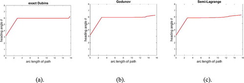
Figure 4. Example 2 (free environment, continued). Plot of heading angle $\theta$ vs arc-length s of Figure 3. (a) Analytical. The heading changes linearly with slope $\frac{\mathrm{v}}{\rho }=1$ along the first (entry) circular arc from initial heading ${\theta }_{\mathrm{A}}$ to the first tangential point heading at ${\mathrm{t}}_{\mathrm{s}\mathrm{w}1}$, then maintains at this heading until another tangential point with the same heading on the final (exit) circular arc at ${\mathrm{t}}_{\mathrm{s}\mathrm{w}2}$, and then another linear change of heading from this tangential point to final heading ${\theta }_{\mathrm{B}}$ at T. the net heading change along the entire path is ${\theta }_{\mathrm{B}}-{\theta }_{\mathrm{A}}.$ (b) Godunov (c) semi-Lagrange.

4.2. Example 2 (Dubins path)

Thanks to the availability of the exact solution of the considered HJB equation, which a closed-form explicit expression is obtained directly as Dubins path, it is possible to compare the influence of numerical HJB solvers derived from necessary optimality condition due to discretization on the quality of each path resulted from both numerical schemes in terms of the accuracy or optimality. In this example, we compare the analytical Dubins path with numerically obtained characteristic line of HJB equation based on numerical value function which has the effect of numerical errors. We are given the initial pose $\left({\mathrm{x}}_{\mathrm{A}},{\mathrm{y}}_{\mathrm{A}},{\theta }_{\mathrm{A}}\right)=\left(-6,6,\pi \right)$and the final pose $\left({\mathrm{x}}_{\mathrm{B}},{\mathrm{y}}_{\mathrm{B}},{\theta }_{\mathrm{B}}\right)=\left(6,0,0\right)$. For numerically solving the modified HJB equation, the 3D uniform (equidistant) Cartesian grid of size $80\times 80\times 80\mathrm{i}\mathrm{s}\mathrm{u}\mathrm{s}\mathrm{e}\mathrm{d},\mathrm{w}\mathrm{h}\mathrm{e}\mathrm{r}\mathrm{e}\mathrm{i}\mathrm{t}\mathrm{h}\mathrm{o}\mathrm{l}\mathrm{d}\mathrm{s}\mathrm{t}\mathrm{h}\mathrm{a}\mathrm{t}{\mathrm{h}}_x={\mathrm{h}}_y=\mathrm{0.25.}$The analytical Dubins path has the length $\rho \pi +\sqrt{160}$.

It could be visualized in Figure 3 that good collision-free trajectories close to the time-optimal trajectory (the analytical Dubins path) are obtained by numerical schemes. Figure 4 shows plots of heading angle $\theta$ vs arc-length s, where it is seen that that the final heading angle is achieved by numerical trajectories. The numerical results also verify that additional necessary optimality conditions for the Dubins path of the type LSL (Techy & Woolsey, 2009) within the families of CSC aforementioned, but here L denotes left (counterclockwise) turn, is the sum of angles of the initial and final circular arcs, each within $\left[0,2\pi \right)$, is less than$2\pi .$ This validates that the solutions obtained by numerical and analytical method are in excellent agreement. Furthermore, the path and length computed by Godunov Hamiltonian scheme is closer and more accurate to the analytical Dubins path than by semi-Lagrange method. And the overall convergence rate of semi-Lagrange scheme is lower than Godunov scheme.

In a cluttered environment of Examples 3 and 4 presented in the following, analytical collision-free Dubins-like paths could be generated via beginning and ending tangential circular arcs and line segments, as an alternative open-loop approach to numerical methods (Liang et al., 2015; Yang et al.; Yang & Kapila, 2002) for comparison. In simulation Examples 3 and 4, by taking advantage of Dubins path as part of collision-free path generation: it follows the boundary of the circular obstacle when in close proximity, and follows the tangential line when between two circles to shorten the path.

Figure 5. Example 3 (cluttered environment). (a) The analytical collision-free path around the obstacle encountered while navigating from initial pose to final pose. It composed of two line segments and one very small contact arc around the obstacle boundary. The length is 16.1258. (b) The level curves (black contours) and the collision-free path (red line) computed with finite set of values of value function at grids obtained by Godunov Hamiltonian scheme. The length is 16.1648. (c) The collision-free path computed with finite set of values of value function at grids obtained by semi-Lagrange scheme. The length is 16.2344, slightly longer. The numerical discretization spacing in x-, y-coordinates is ${\mathrm{h}}_x={\mathrm{h}}_y=0.25$.

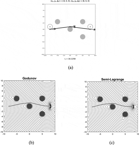
4.3. Example 3 (Time-optimal collision-free path planning)

Same as Example 2, except the initial pose $\left({\mathrm{x}}_{\mathrm{A}},{\mathrm{y}}_{\mathrm{A}},{\theta }_{\mathrm{A}}\right)=\left(-8,0,0\right)$, and the final pose $\left({\mathrm{x}}_{\mathrm{B}},{\mathrm{y}}_{\mathrm{B}},{\theta }_{\mathrm{B}}\right)=\left(8,0,0\right)$. In the absence of obstacles, the Dubins path is the horizontal line segment from$\mathrm{x}=-8\mathrm{t}\mathrm{o}8.$ Suppose there are four circular obstacles of radius 1 with center located at $\left(-5.0,3.0\right)$, $\left(0.0,0.0\right)$, $\left(5.0,3.0\right)$, $\left(5.0,-3.0\right)$, respectively. To compute the collision-avoidance time-optimal trajectory computed by numerically solving the characteristics ODEs of HJB equation, the time step is set as $\mathrm{\Delta }\mathrm{t}=\frac{min\left\{h_x,h_y,h_{\theta }\right\}}{10}$ with ${\mathrm{h}}_x={\mathrm{h}}_y=0.25$. On the other hand, for single circular obstacle avoidance, it suffices to use the tangential lines connections between the initial turning circle and an entrance point on the obstacle circle with radius greater or equal to 1, follow the obstacle boundary to another exit point on the obstacle circle, then exit from this point on the obstacle circle to the goal turning circle (Yang & Kapila, 2002). This analytical path based on geometric construction for this example has the length $2\rho \left(\pi -2\theta \right)+2\sqrt{65-{\left(2\rho \right)}^2}$,where

$\theta =arctan\left(\frac{\sqrt{65-{\left(2\rho \right)}^2}}{2\rho }\right)+{tan}^{-1}\left(\frac{1}{8}\right)$

In Figure 5, we show the numerical collision-free paths and an analytical path for this example, and the evolution of heading change, which depends on the discretization of orientation, along the path is shown in Figure 6.

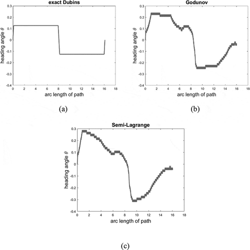
Figure 6. Example 3 (cluttered environment, continued). Plot of the heading angle $\theta$ along the path parametrized arc-length $\mathrm{s}$ of Figure 5. (a) analytical profile: most portions of the path are straight line segments with fixed heading. (b) Godunov scheme. (c) semi-Lagrange scheme. The errors in heading in both numerical schemes are significant, and the heading error propagates through the Dubins vehicle kinematics to the motion. The changes in heading are mostly artifacts resulting from numerical errors.

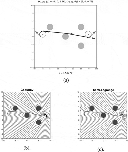
4.4. Example 4 (Planning with nonparallel poses)

Same as Example 3, except a different setting of initial and goal poses. The initial pose is $\left({\mathrm{x}}_{\mathrm{A}},{\mathrm{y}}_{\mathrm{A}},{\theta }_{\mathrm{A}}\right)=\left(-8,0,\frac{3\pi }{4}\right)$ and the goal pose is $\left({\mathrm{x}}_{\mathrm{B}},{\mathrm{y}}_{\mathrm{B}},{\theta }_{\mathrm{B}}\right)=\left(8,0,\frac{\pi }{4}\right)$. We see from Figure 7 that Godunov Hamiltonian scheme finds a path slightly shorter (faster) than the one found by semi-Lagrange scheme, thus closer to the analytical length-minimal (time-optimal) path. The analytical path based on geometric construction has length $\rho \left({\theta }_1+{\theta }_2+{\theta }_3\right)+\sqrt{65-8\sqrt{2}}+\sqrt{61-8\sqrt{2}}$, where

${\theta }_1=\frac{3\pi }{4}+{tan}^{-1}\left(\frac{\sqrt{2}}{16-\sqrt{2}}\right)$

${\theta }_2=\frac{\pi }{2}-{tan}^{-1}\left(\frac{\sqrt{61-8\sqrt{2}}}{2}\right)-2{tan}^{-1}\left(\frac{\sqrt{2}}{16-\sqrt{2}}\right)$

${\theta }_3=\frac{3\pi }{4}-{tan}^{-1}\left(\frac{\sqrt{61-8\sqrt{2}}}{2}\right)-{tan}^{-1}\left(\frac{\sqrt{2}}{16-\sqrt{2}}\right)$

Figure 7 shows the paths obtained analytically and numerically. Figure 8 demonstrates the heading evolution along the analytical Dubins path and the numerically obtained paths in this simulation.

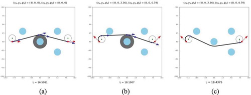
Figure 7. Example 4 (cluttered environment, same as Example 3). (a) The analytical Dubins-like collision-free path around the obstacle. The length is 17.8772. (b) The level curves and the obstacle-avoiding path computed with Godunov Hamiltonian scheme. The length is 17.8946. (c) The level curves and the obstacle-avoiding path computed with semi-Lagrange scheme. The length is 17.9100, slightly longer. The numerical discretization spacing in x-, y-coordinates is ${\mathrm{h}}_x={\mathrm{h}}_y=0.25$.

In practice, suppose the selection of obstacle to be avoided at the current vehicle position is determined. It is advisable to set a safety zone for the obstacle to be avoided to account for the vehicle size and the uncertainties in the detected obstacles, map, control and modeling. To explicitly avoid generating paths that are too close to the obstacle, a clearance is added to augment or dilate the obstacle to enlarge the area that obstacle may occupy so that the distance between the vehicle and the obstacle is kept from a safety zone. The clearance is used to account for the magnitude of uncertainties in obstacle geometry and location sensed by the sensors, inaccuracy in navigation and the vehicle size. To show the effect of setting clearance around the obstacle, two collision-free paths for Example, 3, 4 are shown, respectively, in Figure 9, where the obstacle to be avoided is enlarged by expanding the radius of the obstacles to radius 2.0 for setting a safety margin around the obstacles. We see that the obtained Dubins-like path has a path length a little longer with a larger turn but keeps a larger distance to the obstacle for the benefit of safety. As can be seen, the paths depicted in Figures 5, 7 and 9 composed by the path primitives consisting of circular arcs and line segments respect the safety constraint in clufsttered environment, either following the border of an obstacle or very close to the border of an obstacle when in close proximity to shorten the length, as mentioned previously. In Figure 10, we show another class of valid paths generated with Hybrid A* using the heuristic of Dubins path or Euclidean distance (Dolgov et al., 2008) for Example3 and Example 4 in a cluttered environment. The resulting path generated by Hybrid A* in Example 3 is comparable to Dubins-like path in length since a large portion of the path is straight. However, the path generated by Hybrid A* search method in Example 4 contains more small detours in turning motion due to grid resolution to meet the curvature constraint, thus longer and needs path smoothing for Dubins vehicle. For these examples, the path can be searched within 1–2 s. However, for more accurate search, the computation time dramatically increases.

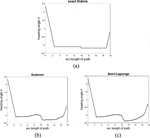
Figure 8. Example 4 (continued). Plot of heading angle $\theta$along the arc-length $\mathrm{s}$ of Figure 6. (a) The analytical profile corresponding to five path segments (three circular arcs and two line segments). (b)Godunov scheme. (c) semi-Lagrange scheme. The largest error in (b), (c) is at the vicinity of obstacle boundary, where heading is to be changed for transition from one path segment to another.

In the case of more complex environment, waypoint navigation of Dubins vehicle is applied so that a UAV visits a sequence of subgoals sequentially (Yang & Kapila, 2002) and remains constant speed between consecutive waypoints to collect or deliver data. The ordering and configuration of the waypoints could be determined a priori, and the desired state (configuration) corresponds to the waypoint to be reached. In our approach of considering only the Dubins-like path, continuously planning Dubins-like path connecting two waypoints could be simply based on Dubins path or applying the numerical approaches based on HJB equation, as we have demonstrated by the above instances of path generation. The computation time increases with the number of waypoints to be traversed by Dubins vehicle. Very recently, in (Chen & Shima, 2019), shortest Dubins paths of 18 types constituted by a concatenation of the successive Dubins paths of CSC or CCC types between two consecutive configurations are derived for passing through three consecutive points with specified initial and terminal headings, where the optimal heading at the intermediate waypoint can be iteratively determined by finding the zero of a polynomial. It is clear that other path primitives such as Bezier curves or B-spline curves (Rousseau et al., 2019), not discussed here, could be employed for waypoint navigation with complex flight trajectories to accomplish different tasks.

Figure 9. Collision-free Dubins-like paths as the obstacle radius is enlarged to 2.0 for maintaining a clearance to the obstacle along the calculated path for (a) Example 3 (b) Example 4, (c) another collision-free Dubins-like path composed by circular arcs and line segments for Example 4. In (a), (b), the generated path contains an arc skirting the clearance circle, i.e. that contacts the boundary of enlarged obstacle.

4.4.1. Remarks on errors sources

The switching structure (i.e. discontinuities of control) of state and control trajectories such as the exact switching time ${\mathrm{t}}_{\mathrm{s}\mathrm{w}2}$ of CSC Dubins path, as evident from Figure 4, is not detected accurately or aligned with the time grids when approximating the bang-singular-bang solutions using state space discretization based numerical methods with fixed time step size for numerical integration using forward Euler method. The error in heading, which ideally is tangent to the path, for numerically obtained trajectory is more evident in Figure 6. A thorough analysis of the overall numerical error should consider several factors: (1) After discretization, the accuracy of numerical methods for the boundary value problem of HJB equation for the approximation of value function is inherently limited by the resolution due to the way in which the gradient of value function is approximated. This is because the Dubins vehicle is allowed to change the values of state, control (i.e. gradient of optimal value function) only at the state space grids and time grids at which the control and path constraints are only enforced, while the constraints may be violated and control switching can occur between the space grids and time grids in real situations. The approximate value function over the entire state space is obtained by interpolation between neighboring grids, thus incurs additional interpolation error (Kang & Wilcox, 2017). Thus, it is essential to apply the higher order more accurate Runge-Kutta method or use a smaller time step size for integrating the Dubins vehicle kinematics to produce more accurate state at a grid for fixed state-space resolution or use more and finer grids for solving HJB equation. (2) The propagation of numerical errors through vehicle motion and constraint sets from the view of computational performance.

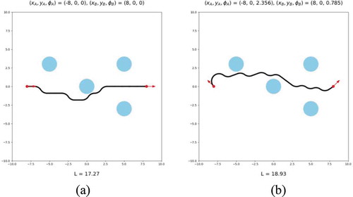
Figure 10. Path generated by Hybrid A* with square grid size 0.25, 16-discrete headings and step size 1 (a) Example 3. The length is 17.27. (b) Example 4. The length is 18.93.

To sum up, due to discretization, only a subset of possible motions is generated and this limits the accuracy, besides the interpolation error and error propagation through the integration of vehicle equation over time. The overall numerical error tendency in Table 1 leads to a general conclusion about accuracy improvement by finer grid resolution, despite the numerical schemes used to compute the time-optimal trajectory. Specifically, Table 1 reveals that a finer grid leads to moderate accuracy improvement for Godunov scheme over the semi-Lagrange scheme. A general strategy is that we can use the information of switching time$\mathrm{s}{\mathrm{t}}_{\mathrm{s}\mathrm{w}1},{\mathrm{t}}_{\mathrm{s}\mathrm{w}2}$ (Section 3.4) obtained during simulations to (re)set the time step or using variable time step size until a satisfactory accuracy (or aggressiveness in our case) is achieved.

5. Conclusion

UAV is an emerging technology, and Dubins vehicle is an ideal kinematic model for constant speed UAV level flight at low constant altitude above ground level in two-dimensional plane. Dubins path is the analytical shortest path between two configurations for a Dubins vehicle. This paper focuses on a class of CSC Dubins-like paths that begin and end with circular arcs of radius not larger than minimum turning radius, precisely composed by a middle line segment connected to tangential circular arcs for heading change at the initial and final configurations. This class of path is feasible for tangent-continuous constrained level flight path generator of constant-speed Dubins vehicle. The path is generated as feedback motion using the approach of HJB equation derived from the necessary condition of time-optimality of state (position and heading) and input (curvature) trajectory in cluttered environment (Takei & Tsai, 2013) modified via Kruzkov transform to tackle with the scaling of the initial condition (such as in the region neighboring the obstacle). The HJB equation approach produces feedback time-optimal control and trajectory, and allows the construction of whole characteristic lines for time-optimal trajectories for any pair of initial-final configurations on a computational domain. For optimal trajectory computing techniques, all of which requires the choice of an analytical method or most often numerical methods. We implement two historical numerical schemes for modified HJB equation to reveal the appropriateness and what resolution of the state, control and time discretization is required for time-optimal trajectory by each numerical scheme. For computational efficiency and path quality, it is seen by a reference to the path produced by Hybrid A* search, the numerical HJB solvers are appropriate. The nearness of trajectories obtained by numerical schemes to the analytical Dubins path of CSC type in a map without obstacles is observed even for a few number of grids, and is enhanced if the grid resolution is finer. Furthermore, Godunov numerical scheme exhibits better performance in generating a position, heading trajectory and curvature profile of Dubins vehicle, guaranteeing collision-free and near time-optimal in cluttered environment. However, to obtain accurate switching structure of time-optimal trajectory that may be essential for some applications, it is observed that in addition to finer grid resolution, time step for generating characteristic lines of Dubins vehicle should be correspondingly smaller than the convergence requirement, preferably taking advantage of the switching time information obtained from the simulations. In the future, it is thus possible to online generate collision-free time-optimal trajectory of Dubins vehicle such as level flight of UAV with optimal state feedback control for more complex scenarios, for example, pursuit-evasion game (such as racing drones) or incorporation of the vehicle motion constraints such as kinodynamic constraints such as vehicle handling limits (velocity and acceleration constraints), in addition to curvature constraint considered in this paper, via HJB equation approach with newest class of faster numerical schemes, and compare with other flyable paths. Furthermore, additional input such as the velocity of Dubins vehicle can be considered (Ben-Asher et al., 2020; Wolek et al., 2016), and complex switching structure can be generated.

Acknowledgements

The authors are grateful to the reviewers’ comments that improve the paper.

Additional information

Funding

This work was supported by the IIS, Academia Sinica [Internal Grant].

Notes on contributors

Jing-Sin Liu

Jing-Sin Liu received his PhD degree from National Taiwan University in 1990. He is an Associate Research Fellow at Institute of Information Science, Academia Sinica, an IEEE Senior Member. The group lead by J.-S. Liu has steadily studied different computational methodologies of path planning for unmanned vehicles. Our work focuses on the nonholonomic path optimization in the presence of obstacles for unicycle or Dubins vehicle subject to curvature constraint. The methodologies employed are fast marching method, fluid dynamics (harmonic functions) method, metaheuristics and numerical nonlinear optimal control including learning-based methods in the presence of uncertainties. This paper is a lasting work on shortest path planning, which is equivalent to time-optimal trajectory planning in the case of constant speed Dubins vehicle, to see if the numerical methods, which is iterative thus expensive in nature, can acquire an accurate solution with a limited time budget.

References

- Aguiar, A. P., Bayer, F. A., Hauser, J., Häusler, A. J., Notarstefano, G., Pascoal, A. M., & Saccon, A. (2017). Constrained optimal motion planning for autonomous vehicles using PRONTO. In Sensing and control for autonomous vehicles (pp. 207–32). Springer.
- Bardi, M., & Capuzzo-Dolcetta, I. (2008). Optimal control and viscosity solutions of Hamilton-Jacobi-Bellman equations. Springer Science and Business Media.
- Ben-Asher, J. Z., Wetzler, M., & Rimon, E. D. (2020). Time optimal trajectories for a mobile robot under nonsliding and radius-of-turn constraints. Journal of Dynamic Systems, Measurement, and Control, 142(6), 11. https://doi.org/10.1115/1.4046331
- Bertolazzi, E., & Frego, M. (2018). Semianalytical minimum‐time solution for the optimal control of a vehicle subject to limited acceleration. Optimal Control Applications & Methods, 39(2), 774–791. https://doi.org/10.1002/oca.2376
- Bokanowski, O., Garcke, J., Griebel, M., & Klompmaker, I. (2013). An adaptive sparse grid semi-Lagrangian scheme for first order Hamilton-Jacobi Bellman equations. Journal of Scientific Computing, 55(3), 575–605. https://doi.org/10.1007/s10915-012-9648-x
- Botkin, N., Hoffmann, K. H., Mayer, N., & Turova, V. (2011). Computation of value functions in nonlinear differential games with state constraints. IFIP conference on system modeling and optimization (pp. 235–244). Berlin, Heidelberg: Springer.
- Bui, X. N., Boissonnat, J. D., Soueres, P., & Laumond, J. P. (1994). Shortest path synthesis for Dubins non-holonomic robot. IEEE International Conference on Robotics and Automation, 1, 2–7. https://doi.org/10.1109/ROBOT.1994.351019
- Castro, A. L., & Koiller, J. (2013). On the dynamic Markov-Dubins problem: From path planning in robotics and biolocomotion to computational anatomy. Regular and Chaotic Dynamics, 18(1–2), 1–20. https://doi.org/10.1134/S1560354713010012
- Chen, Q. Y., Lu, Y. F., Jia, G. W., Li, Y., Zhu, B. J., & Lin, J. C. (2018). Path planning for UAVs formation reconfiguration based on Dubins trajectory. Journal of Central South University, 25(11), 2664–2676. https://doi.org/10.1007/s11771-018-3944-z
- Chen, Z., & Shima, T. (2019). Shortest Dubins paths through three points. Automatica, 105, 368–375. https://doi.org/10.1016/j.automatica.2019.04.007
- Consolini, L., Laurini, M., & Locatelli, M. (2019). Graph-based algorithms for the efficient solution of optimization problems involving monotone functions. Computational Optimization and Applications, 73, 101-128. https://doi.org/10.1007/s10589-019-00070-4
- Crandall, M. G., & Lions, P. L. (1984). Two Approximations of Solutions of Hamilton-Jacobi Equations. Mathematics of Computations, 43(167), 1–19. https://doi.org/10.1090/S0025-5718-1984-0744921-8
- Desaulniers, G. (1996). On shortest paths for a car-like robot maneuvering around obstacles. Robotics and Autonomous Systems, 17(3), 139–148. https://doi.org/10.1016/0921-8890(96)80512-4
- Dolgov, D., Thrun, S., Montemerlo, M., & Diebel, J. (2008). Practical search techniques in path planning for autonomous driving. 1st international symposium search technology and artificial intelligence and robotics, Chicago, USA.
- Dubins, L. E. (1957, July). On curves of minimal length with a constraint on average curvature, and with prescribed initial and terminal positions and tangents. American Journal of Mathematics, 79(3), 497–516. https://doi.org/10.2307/2372560
- Falcone, M. (2013). Recent results in the approximation of nonlinear optimal control problems. International conference on large-scale scientific computing (pp. 15–32). Berlin, Heidelberg: Springer.
- Fedotov, A. A., & Patsko, V. S. (2018). Investigation of reachable set at instant for the Dubins’ car, 58th Israel annual conference on aerospace sciences, IACAS 2018 (pp.1655–1669). Tel-Aviv and Haifa, Israel.
- Ferretti, G., Ferretti, R., Junge, O., & Schreiber, A. (2017). An adaptive multilevel radial basis function scheme for the HJB equation. IFAC-PapersOnLine, 50(1), 1643–1648. https://doi.org/10.1016/j.ifacol.2017.08.331
- Font, R., & Pedregal, P. (2018). Some numerical tests for an alternative approach to optimal feedback control. Journal of the Franklin Institute, 355(15), 7011–7026. https://doi.org/10.1016/j.jfranklin.2018.08.004
- Gong, Q., Lewis, R., & Ross, M. (2009). Pseudospectral motion planning for autonomous vehicles. Journal of Guidance, Control, and Dynamics, 32(3), 1039–1045. https://doi.org/10.2514/1.39697
- Guo, B. Z., & Wu, T. T. (2017). Numerical solution to optimal feedback control by dynamic programming approach: A local approximation algorithm. Journal of Systems Science and Complexity, 30(4), 782–802. https://doi.org/10.1007/s11424-017-5149-1
- Hota, S., & Ghose, D. (2010). Optimal path planning for an aerial vehicle in 3D space. 49th IEEE conference on decision and control (pp. 4902–4907). Atlanta, Georgia, USA.
- Jamhour, E., & Andr’e, P. J. (1996). Planning smooth trajectories along parametric paths. Mathematics and Computers in Simulation, 41(5–6), 615–626. https://doi.org/10.1016/0378-4754(95)00105-0
- Kang, W., & Wilcox, L. C. (2017). Mitigating the curse of dimensionality: Sparse grid characteristics method for optimal feedback control and HJB equations. Computational Optimization and Applications, 68(2), 289–315. https://doi.org/10.1007/s10589-017-9910-0
- Kao, C.-Y., Osher, S., & Qian, J. (2004, May). Lax-Friedrichs sweeping scheme for static Hamilton-Jacobi equations. Journal of Computational Physics, 196(1), 367–391. https://doi.org/10.1016/j.jcp.2003.11.007
- Kaya, C. Y. (2017). Markov-Dubins path via optimal control theory. Computational Optimization and Applications, 68(3), 719–747. https://doi.org/10.1007/s10589-017-9923-8
- Liang, H., Zhong, W., & Chunhui, Z. (2015, July 28). Point-to-point near-optimal obstacle avoidance path for the unmanned aerial vehicle. 34th Chinese control conference, Hangzhou, China.
- Lugo-Cárdenas, I., Flores, G., Salazar, S., & Lozano, R. (2014). Dubins path generation for a fixed wing UAV. IEEE international conference on unmanned aircraft systems (ICUAS), 2014 (pp. 339–346). Wyndham Grand Orlando Resort, Orlando, FL USA.
- Manor, G., Ben-Asher, J. Z., & Rimon, E. (2018). Time optimal trajectories for a mobile robot under explicit acceleration constraints. IEEE Transactions on Aerospace and Electronic Systems, 54(5), 2220–2232. https://doi.org/10.1109/TAES.2018.2811158
- Mehrali-Varjani, M., Shamsi, M., & Malek, A. (2018). Solving a class of Hamilton-Jacobi-Bellman equations using pseudospectral methods. Kybernetika, 54(4), 629–647. https://doi.org/10.14736/kyb-2018-4-0629
- Michael, G. (1983). Crandall and Pierre-Louis Lions, viscosity solutions of Hamilton-Jacobi equations. Transaction of the American Mathematical Society, 277(1), 1–42. https://doi.org/10.1090/S0002-9947-1983-0690039-8
- Patten, W. N., Wu, H. C., & Cai, W. (1994). Perfect parallel parking via Pontryagin’s principle. Journal of Dynamic Systems, Measurement, and Control, 116(4), 723–728. https://doi.org/10.1115/1.2899271
- Pham, Q. C. (2014). A general, fast, and robust implementation of the time-optimal path parameterization algorithm. IEEE Transactions on Robotics, 30(6), 1533–1540. https://doi.org/10.1109/TRO.2014.2351113
- Pharpatara, P., Hérissé, B., & Bestaoui, Y. (2015). 3D-shortest paths for a hypersonic glider in a heterogeneous environment. Workshop on Advanced Control and Navigation for Autonomous Aerospace Vehicles-ACNAAV 2015, 28(9), 186–191. https://doi.org/10.1016/j.ifacol.2015.08.081
- Poonawala, H. A., & Spong, M. W. (2017). Time-optimal velocity tracking control for differential drive robots. Automatica, 85, 153–157. https://doi.org/10.1016/j.automatica.2017.07.038
- Rousseau, G., Maniu, C. S., Tebbani, S., Babel, M., & Martin, N. (2019). Minimum-time B-spline trajectories with corridor constraints. Application to cinematographic quadrotor flight plans. Control Engineering Practice, 89, 190–203. https://doi.org/10.1016/j.conengprac.2019.05.022
- Sundar, S., & Shiller, Z. (1997). Optimal obstacle avoidance based on the Hamilton-Jacobi-Bellman equation. IEEE Transactions on Robotics and Automation, 13(2), 305–310. https://doi.org/10.1109/70.563653
- Szuster, M., & Hendzel, Z. (2018). Optimal control methods for mechatronic systems. In Intelligent optimal adaptive control for mechatronic systems (pp. 61–83). Springer Studies in Systems, Decision and Control.
- Takei, R., & Tsai, R. (2013). Optimal trajectories of curvature constrained motion in the Hamilton-Jacobi formulations. Journal of Scientific Computing, 54(2–3), 622–644. https://doi.org/10.1007/s10915-012-9671-y
- Techy, L., & Woolsey, C. A. (2009). Minimum-time path planning for unmanned aerial vehicles in steady uniform winds. Journal of Guidance, Control, and Dynamics, 32(6), 1736–1746. https://doi.org/10.2514/1.44580
- Tonon, D., Aronna, M. S., & Kalise, D. (2017). Optimal control: Novel directions and applications. Springer lecture notes in mathematics 2180.
- Tsai, Y.-H. R., Cheng, L.-T., Osher, S., & Zhao, H.-K. (2017). Fast sweeping algorithms for a class of Hamilton-Jacobi equations. SIAM Journal on Numerical Analysis, 41(2), 673–694. https://doi.org/10.1137/S0036142901396533
- Tsourdos, A., White, B., & Shanmugavel, M. (2010). Cooperative path planning of unmanned aerial vehicles. John Wiley and Sons.
- Wang, S., Gao, F., & Teo, K. L. (2000). An upwind finite-difference method for the approximation of viscosity solutions to Hamilton-Jacobi-Bellman equations. IMA Journal of Mathematical Control and Information, 17(2), 167–178. https://doi.org/10.1093/imamci/17.2.167
- Wolek, A., & Woolsey, C. A. (2017). Model-based path planning. In Sensing and control for autonomous vehicles (pp. 183–206). Springer lecture notes in control and information sciences, 474.
- Wolek, A., Cliff, E. M., & Woolsey, C. A. (2016). Time-optimal path planning for a kinematic car with variable speed. Journal of Guidance, Control, and Dynamics, 39(10), 2374–2390. https://doi.org/10.2514/1.G001317
- Wu, W., Chen, H., & Woo, P. Y. (2000). Time optimal path planning for a wheeled mobile robot. Journal of Robotic Systems, 17(11), 585–591. https://doi.org/10.1002/1097-4563(200011)17:11<585::AID-ROB1>3.0.CO;2-7
- Yang, D., Li, D., & Sun, H. 2D Dubins path in environment with obstacle. Mathematical Problems in Engineering, 2013. https://doi.org/10.1155/2013/291372
- Yang, G., & Kapila, V. (2002). Optimal path planning for unmanned air vehicles with kinematic and tactical constraints. 41st IEEE conference on decision and control (pp. 1301–1306), Las Vegas, NV, USA.
- Zdesar, A., & Škrjanc, I. (2018, January). Optimum velocity profile of multiple Bernstein-Bézier curves subject to constraints for mobile robots. ACM Transactions on Intelligent Systems and Technology 9(5). Article No. 56. https://doi.org/10.1145/3183891
- Zhakatayev, A., Rubagotti, M., & Varol, H. A. (2017). Time-optimal control of variable-stiffness-actuated systems. IEEE/ASME Transactions on Mechatronics, 22(3), 1247–1258. https://doi.org/10.1109/TMECH.2017.2671371
- Zhao, H. (2005). A fast sweeping method for Eikonal equations. Mathematics of Computation, 74(250), 603–627. https://doi.org/10.1090/S0025-5718-04-01678-3
- Zhao, H. (2016). The fast sweeping method for stationary Hamilton-Jacobi equations. In Handbook of numerical analysis chapter 22 (Vol. 17, pp. 585–601), Science Direct.
- Zhu, J., Trélat, E., & Cerf, M. (2017). Geometric optimal control and applications to aerospace. Pacific Journal of Mathematics for Industry, 9(8), 41. https://doi.org/10.1186/s40736-017-0033-4
- Zollars, M. D., Cobb, R. G., & Grymin, D. J. (2018). Simplex optimal control methods for urban environment path planning. 2018 AIAA information systems-AIAA Infotech@ aerospace (pp. 16), Kissimmee, Florida, USA.