Spatio-temporal characteristics of fertilizer utilization efficiency in China during 1999-2018: a biennial weight modified Russell model

Abstract

The excessive application of fertilizer in China’s agricultural production increases the planting cost, whilst leading to the deterioration of ecological environment. It is therefore of great significance to evaluate China’s fertilizer utilization efficiency (FUE) for agricultural sustainability. However, in spite of its importance in China’s agriculture system, the relevant literature is still scarce. To fill this gap, this study examines the FUE and its spatio-temporal characteristics in China by employing a biennial weight modified Russell model. The main findings are as follows. First, the FUE of China and the three functional areas for grain production fluctuated downward during the sample period. The mean FUE in the main grain-selling areas (0.9856) was the highest, followed by the grain balance areas (0.7843), and then the main grain-producing areas (0.7499). Second, there were 15 provinces with a mean FUE above 0.9. Shanghai (0.9981), Tibet (0.9976), Hainan (0.9975), and Beijing (0.9958) were the top four provinces regarding mean FUEs. Anhui (0.4867) and Shanxi (0.4778) had the lowest mean FUEs. Third, the total difference within China was increased by 31.8% over the sample period. The intra-regional contribution, the net inter-regional contribution, and the inter-regional intensity of transvariation accounted for 29.5%, 43.4%, and 27.11% of the total difference.

Keywords:

• fertilizer
• efficiency
• data envelopment analysis

1. Introduction

Agriculture is the national economic base, particularly in China. Since China’s reform and opening-up, its agriculture system has undergone a historical transition, creating the miracle of feeding 20% of the world’s population with less than 9% of the world’s arable land area (Guan et al., 2016). China’s agricultural gross domestic product grew from 101.846 billion yuan in 1978 to 8,308.6 billion yuan in 2021, showing an average annual growth rate of over 10 percent. According to China Rural Statistical Yearbook, the total grain output rose from 304.765 million tons in 1978 to 682.85 million tons in 2021, showing an average annual growth rate of around 1.9 percent.¹ However, the long-term growth of Chinese agriculture is at the cost of high input factors, high waste of resources, and high emission of pollutants (Ren et al., 2021). The rising costs of labor and other factors, the increasing constraints of resources, and the progressively severe environmental pollution form significant barriers to the green development of agriculture (Huang et al., 2019; Xu et al., 2022b).

Fertilizers play a key role in ensuring the adequate supply of agricultural products and thus improving food security (Chukalla et al., 2020; Hellegers & van Halsema, 2021; Pronger et al., 2019). China consumes 35 percent of the world’s fertilizer (S. Zhang et al., 2022). Food and Agriculture Organization of the United Nations showed that China consumed 503.32 kg of fertilizer per hectare in 2016, about 3.58 times the world average of 140.55 kg (H. Liu et al., 2019). From 1979 to 2019, China’s fertilizer use increased from 10.86 million tons to 54.04 million tons, with an average annual growth rate of 4.1 percent. Excessive use of fertilizer increases the planting cost and leads to the deterioration of the ecological environment. In 2021, the Chinese central government called for continuous efforts to reduce the applied amount of fertilizer and increase its efficiency. Due to a vast territory with diverse climate and various soil types and uneven economic levels, there are significant spatial disparities in fertilizer utilization efficiency in China. That is unfavorable to controlling agricultural environmental pollution and thus hinders the coordinated implementation of policies to increase efficiency. Therefore, this paper examines the temporal and spatial characteristics of China’s fertilizer utilization efficiency (FUE), which is of great significance to accurately formulate regional fertilizer policies in order to narrow the differences of FUEs and promote the coordinated development of agricultural regions.

Most prior studies focus on agricultural total factor productivity (Guo & Liu, 2020; Hoang & Coelli, 2011; Huang et al., 2022; Xu et al., 2022a). The indicator measures the efficiency of all inputs. It is also a research framework that can be used to measure the efficiency of single factors, such as total factor energy productivity. Under the framework of the total factor productivity, many scholars have conducted research on single factor productivity, mainly focusing on labor efficiency, energy, and carbon efficiency (Long et al., 2018; J. X. Liu et al., 2021b; G. Y. Wu et al., 2022; J. Yang et al., 2016a; Zhang et al., 2019; Zheng et al., 2021). Long et al. (2018) investigated the environmental efficiency of China’s agriculture and its determinants during 1997–2014. G. Y. Wu et al. (2022) measured the agricultural eco-efficiency of China from the perspective of eco-civilization construction, agricultural nonpoint source pollution emissions, and carbon emissions. Fertilizer received little attention. Some studies used the terms total factor energy efficiency and total factor carbon productivity to refer to energy efficiency and carbon efficiency under the framework of total factor productivity (Borozan, 2018; Hu & Xiong, 2021; Li et al., 2018; Lin & Tan, 2016; Ohene-Asare et al., 2020). Measuring FUE in this study is also under the framework.

The existing literature mainly employs the production frontier theory to explore China’s FUE. This theory has two main approaches, stochastic frontier analysis (SFA) and data envelopment analysis (DEA). SFA is a parametric approach that sets the function form of frontier production technology and the distribution form of random terms in a parameter way in advance (Aigner et al., 1977; Granderson, 1997; Kumbhakar et al., 2000; Nishimizu & Page, 1982). However, SFA cannot consider the constraints of resources and environment, and the incorrect setting of its function form significantly affects the correctness of the results (Battese & Coelli, 1995; Greene, 2010; Habib & Ljungqvist, 2005). DEA, a nonparametric efficiency evaluation method, does not need to assure the form of the production function, and its result is endogenous from the data. Hence, DEA can avoid the deviation caused by the function setting. More importantly, it can incorporate undesirable outputs into the efficiency measurement framework. Therefore, it has become the primary method of evaluating green efficiency or green productivity, and this study also employs a DEA model. The traditional DEA is more sensitive to outliers than SFA because it relies too much on data. In addition, there is an infeasibility problem when solving DEA models. The occurrence of infeasibility is closely related to data characteristics (Fujii et al., 2014). However, we can take some measures to solve the above two problems.

DEA model has many sub-models, including three-stage DEA (Chao, 2017), inverse DEA (Lim, 2016), the meta-frontier DEA (Zhang et al., 2013), Chance-constrained DEA (Land et al., 1993), and the network DEA (Losa et al., 2020). The most suitable model should be selected according to the specific purpose (Rebolledo-Leiva et al., 2017; Yaqubi et al., 2016). Y. Yang et al. (2016b) employed the dynamic DEA model to calculate the environmental efficiency of corn production in Northeast China from 2005 to 2013 and found excessive fertilizer use. Wang et al. (2017) used the traditional DEA model to evaluate the fertilizer efficiency in the arid area of northwest China. They found that the application of fertilizer in this area could be reduced by 41.53%. Based on the panel data of 63 counties in Zhejiang from 2003 to 2017, Yang and Lin (2020) investigated the total factor substitution efficiency and its Spatio-temporal evolution of fertilizer input by the super-efficiency DEA model, locational Gini coefficient, and Tihl index. Some researchers measure FUE from other perspectives. Yadav (2003) and Gabriel et al. (2016) measure FUE based on farm pilot areas. Their disadvantage is that the trial area is limited and cannot be extended to the entire region.

However, several aspects of existing research can be further argued. First, the prior research seldom considers the undesired output when constructing the measurement framework of FUE. There is no consistent standard to select carbon emission sources. It is only ensured that the closer the calculated carbon emissions are to the actual values, the better the results for the model. Y. Yang et al. (2016b) included agricultural carbon emissions into the calculation framework as an undesirable output, but the calculation of agricultural carbon emissions was inaccurate. Second, the previous studies always tended to divide China into three regions from the perspective of geography: eastern, central, and western. Hitherto, little attention has been paid to the analysis of FUE from the perspective of functional areas for grain production, including main grain-producing areas (MGPAs), grain balance areas (GBAs), and main grain-selling areas (MGSAs).²

This study employs a biennial weight modified Russell model (BWMRM) to investigate China’s FUE and the spatio-temporal characteristics. The main contribution of this study includes the following three aspects. First, this study selects various agricultural carbon emission sources, while fully considering their heterogeneity. Straw burning is one of the carbon sources, to which very little attention has been paid. Burning different kinds of straw has different carbon intensity. Moreover, the carbon intensity of rice farming depends not only on the variety of rice (early rice, late rice, in-season rice), but also on the area where it is grown. In addition, the carbon intensity of the soil surface is also related to the type of crops grown on the soil. These scenarios are adequately taken into account in this study. Second, the study divides China into three regions based on their grain production: MGPAs, GBAs and MGSAs. Hence, the spatial heterogeneity of FUE in these regions can be investigated. Third, this study used the biennial environmental production technology to build a BWMRM which can reduce the impact of outliers and solve the infeasibility. This model has rarely been adopted in empirical analysis. This study is the first endeavor to employ BWMRM in examining FUE. Although the global frontier, a recently developed DEA approach, was widely used to address infeasibility, it was found ineffective (G. Liu et al., 2016).

2. Materials and methods

2.1. Data source

The sample includes data from 31 provinces in China (excluding Hong Kong, Macao, and Taiwan) from 1999 to 2018, obtained from the China Rural Statistical Yearbook, the China Agricultural Yearbook, and the China Animal Husbandry and Veterinary Yearbook.³

2.2. The selection of input and output indicators

Measuring FUE requires input and output indicators, which are shown in Table 1.

Table 1. Construction of input and output indicators

	Factor	Indicator
Input	Labor (L)	The number of agricultural practitioners (unit: million)
	Land (N)	Area sown with crops (unit: hectare)
	Machinery (E)	Electricity consumption of agricultural machinery (unit: kilowatts)
	Fertilizer (F)	Applying quantity of chemical fertilizer (unit: ton)
	Pesticide (P)	Consumption of chemical pesticides (unit: ton)
	Agricultural film (R)	The amount of agricultural film used (unit: ton)
	Agricultural water (W)	Actual irrigation area (unit: hectare)
	Farm animals (A)	The number of farm draft animals (unit: million)
Output	Desirable output (Y)	The actual agricultural production (Yuan)
	Undesirable output (C)	Agricultural carbon emissions (ton)

In this study, the agricultural carbon emission sources include five categories: (1) agricultural materials; (2) rice cultivation⁴; (3) soil surface releasing when planting crops; (4) livestock and poultry farming⁵; (5) straw burning. The five also include a variety of sub-sources, as shown in Table 2. Using carbon emission coefficients and conversion coefficients, we can convert the amount of agricultural carbon emission sources into carbon emissions. The specific calculation method of agricultural carbon emissions was according to Huang et al. (2019).

Table 2. Agricultural carbon emission sources

Sources	Sub-sources
Agricultural materials	Fertilizer, pesticides, plastic sheeting, diesel oil, and energy consumption for irrigation
Rice cultivation	Early rice, late rice, in-season rice
Soil Surface releasing when planting crops	Paddy rice, winter wheat, spring wheat, soybean, corn, and vegetables
Livestock and poultry farming	Cow, buffalo, cattle, mule, camel, donkey, horse, pig, sheep, goat, rabbit, and poultry
Straw burning	Rice, wheat, corn, rape, soybean, and cotton straw

2.3. BWMRM

Unlike other environmental technologies, such as the global frontier and sequential frontier, the biennial environmental production technology uses two-period decision-making units (DMUs) to construct the production frontier (Pastor et al., 2011; Shestalova, 2003). The technology is shown as Eq. (1)(1) $\begin{array}{c}\left.\sum _{j=1}^n{z}_j^t{b}_{jf}^t+\sum _{j=1}^n{z}_j^{t+1}{b}_{jf}^{t+1}=b_{jf},\sum _{j=1}^n{z}_j=1,z_j\ge 0;\mathrm{\forall }n,i,r,f\right\}\end{array}$(1) . $x$, $y,$ and $b$ denote inputs, desirable outputs, and undesirable outputs, respectively. For DMU $j$ $\left(j=1\dots n\right)$ in period $t\left(t=1\dots T\right)$, its input-output set is $\left(x^{j,t},y^{j,t},b^{j,t}\right)$, and $z$ is the intensity variable. $\sum _{j=1}^n{z}_j=1$ and $z_j\ge 0$ means variable returns to scale (VRS). According to Eq. (1(1) $\begin{array}{c}\left.\sum _{j=1}^n{z}_j^t{b}_{jf}^t+\sum _{j=1}^n{z}_j^{t+1}{b}_{jf}^{t+1}=b_{jf},\sum _{j=1}^n{z}_j=1,z_j\ge 0;\mathrm{\forall }n,i,r,f\right\}\end{array}$(1) ), technical regression may exist, different from the global and sequential frontier. Weak disposability, null-jointness, and the compact set, the three classic assumptions in productivity theory, are met.

$T=\left\{\left(x,y,b\right):\sum _{j=1}^n{z}_j^t{x}_{ji}^t+\sum _{j=1}^n{z}_j^{t+1}{x}_{ji}^{t+1}\le x_{ji},\sum _{j=1}^n{z}_j^t{y}_{jr}^t+\sum _{j=1}^n{z}_j^{t+1}{y}_{jr}^{t+1}\ge y_{jr},\right.$

(1) $\begin{array}{c}\left.\sum _{j=1}^n{z}_j^t{b}_{jf}^t+\sum _{j=1}^n{z}_j^{t+1}{b}_{jf}^{t+1}=b_{jf},\sum _{j=1}^n{z}_j=1,z_j\ge 0;\mathrm{\forall }n,i,r,f\right\}\end{array}$(1)

Chen et al. (2015) introduced the weighted Russell directional distance model (WRDDM) based on the directional Russell measure of inefficiency proposed by Fukuyama and Weber (2009). WRDDM can measure the contribution of each factor (input, output, and undesirable output) to the total inefficiencies, as shown in Eq. (2)(2) $z_j\ge 0;s_{j{ }^{\mathrm{\prime }}{y}_q}^t\ge 0;s_{j{ }^{\mathrm{\prime }}{b}_h}^t\ge 0;s_{j{ }^{\mathrm{\prime }}{x}_m}^t\ge 0;\sum _{j=1}^J{z}_j^t=1;J=1\dots .J.t=1,2,\dots ,T$(2) . Therefore, the model can determine the efficiency of each factor under the framework of total factor productivity, which is the core logic of FUE measurement in this paper. In addition, in the multiple inputs, desirable outputs, and undesirable outputs case, it can identify all the nonzero slacks associated with the input and output constraints and set weights on the contribution of these factors to the total inefficiencies.

${\vec{D}}_{j{ }^{\mathrm{\prime }}V}^{Rt}\left(x^t,y^t,b^t;g^t\right)={\beta }_{j{ }^{\mathrm{\prime }}t}^{Rt}=max{w}_x\left(\sum _{m=1}^M\frac{w_m^x{s}_{j{ }^{\mathrm{\prime }}{x}_m}^t}{g_{j{ }^{\mathrm{\prime }}{x}_m}^t}\right)+w_y\left(\sum _{q=1}^Q\frac{w_q^y{s}_{j{ }^{\mathrm{\prime }}{y}_q}^t}{g_{j{ }^{\mathrm{\prime }}{y}_q}^t}\right)+w_b\left(\sum _{h=1}^H\frac{w_h^b{s}_{j{ }^{\mathrm{\prime }}{b}_h}^t}{g_{j{ }^{\mathrm{\prime }}{b}_h}^t}\right)$

$s.t.$

$\sum _{j=1}^J{z}_j^t{x}_{jm}^t\le x_{j{ }^{\mathrm{\prime }}m}^t-s_{j{ }^{\mathrm{\prime }}{x}_m}^t,for\mathrm{\forall }m=1,2,\dots ,M$

$\sum _{j=1}^J{z}_j^t{y}_{jq}^t\ge y_{j{ }^{\mathrm{\prime }}q}^t+s_{j{ }^{\mathrm{\prime }}{y}_q}^t,for\mathrm{\forall }q=1,2,\dots ,Q$

$\sum _{j=1}^J{z}_j^t{b}_{jh}^t=b_{j{\hspace{0.17em}}_{\hspace{0.17em}}^{\prime }h}^t-s_{j{\hspace{0.17em}}_{\hspace{0.17em}}^{\prime }{b}_h^{\hspace{0.17em}}}^t,\hspace{0.17em}for\hspace{0.17em}\mathrm{\forall }h=1,2,\dots ,H$

(2) $z_j\ge 0;s_{j{ }^{\mathrm{\prime }}{y}_q}^t\ge 0;s_{j{ }^{\mathrm{\prime }}{b}_h}^t\ge 0;s_{j{ }^{\mathrm{\prime }}{x}_m}^t\ge 0;\sum _{j=1}^J{z}_j^t=1;J=1\dots .J.t=1,2,\dots ,T$(2)

BWMRM is based on the biennial environmental production technology and WRDDM. Hence, it has all their advantages. First, it is more flexible because the model does not need to be recomputed completely when one or more periods have been added to the original sample period. Second, it can avoid the infeasibility problem, an important issue when establishing a DEA model. Third, it can determine each factor’s inefficiency performance by setting their weight. Before specifying the specific weights, the combination of the biennial environmental production technology and WRDDM is a nonradial and non-directional biennial generalized directional distance function, as shown in Eq. (3)(3) $\begin{array}{c}{z}_j\hspace{0.17em}\ge 0;s_{j{ }^{\mathrm{\prime }}{y}_q}^{Bt}\ge 0;s_{j{ }^{\mathrm{\prime }}{b}_h}^{Bt}\ge 0;s_{j{ }^{\mathrm{\prime }}{x}_m}^{Bt}\ge 0;\sum _{j=1}^J{z}_j^t+\sum _{j=1}^J{z}_j^{t+1}=1;J=1\dots .J.t=1,2,\dots ,T\end{array}$(3) . Fourth, the model can reduce the impact of outliers and yield a robust result. There are two points in the model that illustrate this advantage. On the one hand, the weight is not endogenous and needs to be set subjectively. Therefore, for robustness, this study has two sets of weights. Like most studies, we consider inputs, desirable, and undesirable outputs as three categories of factors and assign the first set of weights. Meanwhile, we merge the desired and undesired output into one factor (output) category, then give the second set of weights. Finally, the inefficiencies under the two weights are averaged as the objective function for the robustness. Eq. (3)(3) $\begin{array}{c}{z}_j\hspace{0.17em}\ge 0;s_{j{ }^{\mathrm{\prime }}{y}_q}^{Bt}\ge 0;s_{j{ }^{\mathrm{\prime }}{b}_h}^{Bt}\ge 0;s_{j{ }^{\mathrm{\prime }}{x}_m}^{Bt}\ge 0;\sum _{j=1}^J{z}_j^t+\sum _{j=1}^J{z}_j^{t+1}=1;J=1\dots .J.t=1,2,\dots ,T\end{array}$(3) is for DMU $j$ in period $t$ with VRS under the biennial environmental production technology in period $t$. Superscript $B$ means the biennial environmental technology is employed, and subscript $V$ means VRS. Then, we can obtain FUE according to Eq. (4)(4) $\begin{array}{c}FU{E}_{jt}^{Bt}=\frac{F_j^t-s_{j{ }^{\mathrm{\prime }}}^{Bt}}{F_j^t}\end{array}$(4) . On the other hand, the biennial environmental production technology uses DMUs of two adjacent periods to form the production frontier. For instance, $FU{E}_{jt}^{Bt}$ is based on the biennial technology in period $t$ which uses observations of DMUs in periods $t$ and $t+1$. DMU $j$ in period $t$ is involved in constructing the production frontier in period $t-1$, too. Hence, for DMU $j$ in period $t$ under the biennial environmental production technology in period $t-1$, the model can be shown as Eq. (5)(5) $\begin{array}{c}{z}_j\ge 0;s_{j{ }^{\mathrm{\prime }}{y}_q}^{Bt-1}\ge 0;s_{j{ }^{\mathrm{\prime }}{b}_h}^{Bt-1}\ge 0;s_{j{ }^{\mathrm{\prime }}{x}_m}^{Bt-1}\ge 0;\sum _{j=1}^J{z}_j^t+\sum _{j=1}^J{z}_j^{t-1}=1;J=1\dots .J.t=1,2,\dots ,T\end{array}$(5) . In addition, the corresponding FUE is shown as Eq. (6)(6) $\begin{array}{c}FU{E}_{jt}^{Bt-1}=\frac{F_j^t-s_{j{ }^{\mathrm{\prime }}}^{Bt-1}}{F_j^t}\end{array}$(6) . Like the Malmquist productivity index, the study considers the geometrical mean of $FU{E}_{jt}^{Bt}$ and $FU{E}_{jt}^{Bt-1}$ as FUE of DMU $j$ in period $t$, which can improve the robustness of the result, shown as Eq. (7)(7) $\begin{array}{c}FU{E}_{jt}={\left(FU{E}_{jt}^{Bt}\ast FU{E}_{jt}^{Bt-1}\right)}^{0.5}\end{array}$(7) . As with most DEA models, there is no indication of statistical significance in this model.

The biennial generalized directional distance function can be transformed into a variety of models by the direction vector $g_{j{ }^{\mathrm{\prime }}}^t=\left(g_{j{ }^{\mathrm{\prime }}{x}_m}^t,g_{j{ }^{\mathrm{\prime }}{y}_q}^t,g_{j{ }^{\mathrm{\prime }}{b}_h}^t\right)$. When $g_{j{ }^{\mathrm{\prime }}}^t=\left(x_{j{ }^{\mathrm{\prime }}{x}_m}^t,y_{j{ }^{\mathrm{\prime }}{y}_q}^t,b_{j{ }^{\mathrm{\prime }}{b}_h}^t\right)$, this generalized model is BWMRM. This direction vector makes each factor’s inefficiency equal to the ratio of its slack to its original value and has been employed by many studies (Liu & Feng, 2019; G. Liu et al., 2016; G. Wu et al., 2019). According to Fujii et al. (2014) and Chen et al. (2015), this paper alternatively specifies the $\left(w_{1x},w_{1y},w_{1b}\right)$ as $\left(1/3,1/3,1/3\right)$ and $\left(w_{2x},w_{2y}\right)$ as $\left(1/2,1/2\right)$. The internal weight of a category of factor is the reciprocal of the number of subfactors, Hence, $\left(w_m^{1x},w_q^{1y},w_h^{1b}\right)$ is equal to $\left(1/M,1/Q,1/H\right)$ and $\left(w_m^{2x},w_q^{2y},w_h^{2b}\right)$ $\left(1/M,1/\left(Q+H\right),1/\left(Q+H\right)\right)$.

${\overrightarrow{D}}_{j^{\prime }V}^{Bt}\left(x^t,y^t,b^t;g^t\right)={\beta }_{j^{\prime }V}{ }^{Bt}=\max \frac{1}{2}{w}_{1x}\sum m=1M{w}_m^{1x}sj\prime x_{m}Btgj\prime x_{m}t+w_{1y}\sum q=1Q{w}_q^{1y}sj\prime y_{q}Btgj\prime y_{q}t++w_{1b}\sum h=1H{w}_h^{1b}sj\prime b_{h}Btgj\prime b_{h}t+\frac{1}{2}{w}_{2x}\sum m=1M{w}_m^{2x}sj\prime x_{m}Btgj\prime x_{m}t+w_{2y}\sum q=1Q{w}_q^{2y}sj\prime y_{q}Btgj\prime y_{q}t+\sum h=1H{w}_h^{2b}sj\prime b_{h}Btgj\prime b_{h}t]$s.t.

$\sum _{j=1}^J{z}_j^t{x}_{jm}^t+\sum _{j=1}^J{z}_j^{t+1}{x}_{jm}^{t+1}\le x_{j{ }^{\mathrm{\prime }}m}^t-s_{j{ }^{\mathrm{\prime }}{x}_m}^{Bt},for\mathrm{\forall }m=1,2,\dots ,M$

$\sum _{j=1}^J{z}_j^t{y}_{jq}^t+\sum _{j=1}^J{z}_j^{t+1}{y}_{jq}^{t+1}\ge y_{j{ }^{\mathrm{\prime }}q}^t+s_{j{ }^{\mathrm{\prime }}{y}_q}^{Bt},for\mathrm{\forall }q=1,2,\dots ,Q$

$\sum _{j=1}^J{z}_j^t{b}_{jh}^t+\sum _{j=1}^J{z}_j^{t+1}{b}_{jh}^{t+1}=b_{j{\hspace{0.17em}}_{\hspace{0.17em}}^{\prime }h}^t-s_{j{\hspace{0.17em}}_{\hspace{0.17em}}^{\prime }{b}_h^{\hspace{0.17em}}}^{Bt},\hspace{0.17em}for\hspace{0.17em}\mathrm{\forall }h=1,2,\dots ,H$

(3) $\begin{array}{c}{z}_j\hspace{0.17em}\ge 0;s_{j{ }^{\mathrm{\prime }}{y}_q}^{Bt}\ge 0;s_{j{ }^{\mathrm{\prime }}{b}_h}^{Bt}\ge 0;s_{j{ }^{\mathrm{\prime }}{x}_m}^{Bt}\ge 0;\sum _{j=1}^J{z}_j^t+\sum _{j=1}^J{z}_j^{t+1}=1;J=1\dots .J.t=1,2,\dots ,T\end{array}$(3)

(4) $\begin{array}{c}FU{E}_{jt}^{Bt}=\frac{F_j^t-s_{j{ }^{\mathrm{\prime }}}^{Bt}}{F_j^t}\end{array}$(4)

${\overrightarrow{D}}_{j^{\prime }V}^{Bt-1}\left(x^t,y^t,b^t;g^t\right)={\beta }_{j^{\prime }V}{ }^{Bt-1}=\max \frac{1}{2}{w}_{1x}\sum m=1M{w}_m^{1x}sj\prime x_{m}Btgj\prime x_{m}t+w_{1y}\sum q=1Q{w}_q^{1y}sj\prime y_{q}Btgj\prime y_{q}t++w_{1b}\sum h=1H{w}_h^{1b}sj\prime b_{h}Btgj\prime b_{h}t+\frac{1}{2}{w}_{2x}\sum m=1M{w}_m^{2x}sj\prime x_{m}Btgj\prime x_{m}t+w_{2y}\sum q=1Q{w}_q^{2y}sj\prime y_{q}Btgj\prime y_{q}t+\sum h=1H{w}_h^{2b}sj\prime b_{h}Btgj\prime b_{h}t]$s.t.

$\sum _{j=1}^J{z}_j^t{x}_{jm}^t+\sum _{j=1}^J{z}_j^{t-1}{x}_{jm}^{t-1}\le x_{j{ }^{\mathrm{\prime }}m}^t-s_{j{ }^{\mathrm{\prime }}{x}_m}^{Bt-1},for\mathrm{\forall }m=1,2,\dots ,M$

$\sum _{j=1}^J{z}_j^t{y}_{jq}^t+\sum _{j=1}^J{z}_j^{t-1}{y}_{jq}^{t-1}\ge y_{j{ }^{\mathrm{\prime }}q}^t+s_{j{ }^{\mathrm{\prime }}{y}_q}^{Bt-1},for\mathrm{\forall }q=1,2,\dots ,Q$

$\sum _{j=1}^{{ }^J}{z}_j^t{b}_{jh}^t+\sum _{j=1}^J{z}_j^{t-1}{b}_{jh}^{t-1}=b_{j{\hspace{0.17em}}_{\hspace{0.17em}}^{\prime }h}^t-s_{j{\hspace{0.17em}}_{\hspace{0.17em}}^{\prime }{b}_h^{\hspace{0.17em}}}^{Bt-1},\hspace{0.17em}for\hspace{0.17em}\mathrm{\forall }h=1,2,\dots ,H$

(5) $\begin{array}{c}{z}_j\ge 0;s_{j{ }^{\mathrm{\prime }}{y}_q}^{Bt-1}\ge 0;s_{j{ }^{\mathrm{\prime }}{b}_h}^{Bt-1}\ge 0;s_{j{ }^{\mathrm{\prime }}{x}_m}^{Bt-1}\ge 0;\sum _{j=1}^J{z}_j^t+\sum _{j=1}^J{z}_j^{t-1}=1;J=1\dots .J.t=1,2,\dots ,T\end{array}$(5)

(6) $\begin{array}{c}FU{E}_{jt}^{Bt-1}=\frac{F_j^t-s_{j{ }^{\mathrm{\prime }}}^{Bt-1}}{F_j^t}\end{array}$(6)

(7) $\begin{array}{c}FU{E}_{jt}={\left(FU{E}_{jt}^{Bt}\ast FU{E}_{jt}^{Bt-1}\right)}^{0.5}\end{array}$(7)

2.4. Kernel density estimation

As one of the nonparametric estimation methods, the Kernel density is mainly applicable to the probability density estimation of random variables. Suppose the density function of the random variable $X$ is:

(8) $\begin{array}{c}f\left(x\right)=\frac{1}{Nh}\sum _{i=1}^{N}K\left(\frac{X_i-x}{h}\right)\end{array}$(8)

$N$ is the number of observed values, and $X_i$ is the observed value. Each $X_i$ is independent of the other and has an identical distribution. $K$ is the kernel function, and $h$ is the window width. The kernel function $K$ is a weighting function or smooth conversion function, which should meet the requirements, as shown in Eq. (9)(9) $\begin{array}{c}\left\{\begin{array}{c}\underset{x\to \mathrm{\infty }}{lim}K\left(x\right)\cdot x=0\\ K\left(x\right)\ge 0\hspace{0.17em}{\int }_{-\mathrm{\infty }}^{+\mathrm{\infty }}K\left(x\right)dx=1\\ supK\left(x\right)<+\mathrm{\infty }\hspace{0.17em}{\int }_{-\mathrm{\infty }}^{+\mathrm{\infty }}K{\left(x\right)}^{2}dx<+\mathrm{\infty }\end{array}\right\}\end{array}$(9) . Commonly used kernel functions include Gaussian, Triangle, Quaritic, and Epanechnikov, and this study chooses Gaussian (Quah, 1993).

(9) $\begin{array}{c}\left\{\begin{array}{c}\underset{x\to \mathrm{\infty }}{lim}K\left(x\right)\cdot x=0\\ K\left(x\right)\ge 0\hspace{0.17em}{\int }_{-\mathrm{\infty }}^{+\mathrm{\infty }}K\left(x\right)dx=1\\ supK\left(x\right)<+\mathrm{\infty }\hspace{0.17em}{\int }_{-\mathrm{\infty }}^{+\mathrm{\infty }}K{\left(x\right)}^{2}dx<+\mathrm{\infty }\end{array}\right\}\end{array}$(9)

2.5. Dagum Gini ratio

Traditional indicators measuring inequality, such as Theil index and Gini ratio, are built on the assumption of normal distribution and homoscedasticity, which strictly limits the non-overlap between grouped samples and makes it difficult to decompose into several sub-indices with reasonable economic meaning. Dagum (1998) proposed the Dagum Gini ratio in response to these deficiencies, which can decompose the overall difference of samples into three parts: intra-group difference, net inter-group difference, and inter-group intensity of transvariation, and has been widely used. Specifically, the following inter-group Gini ratio is:

(10) $G_{jh}=\frac{{\sum }_{i=1}^{n_j}\hspace{0.17em}{\sum }_{r=1}^{n_h}\hspace{0.17em}\left|y_{ji}-y_{hr}\right|}{n_j{n}_h\left(\hspace{0.17em}{\bar{y}}_j+\hspace{0.17em}{\bar{y}}_h\right)}\hspace{0.17em}$(10)

$G_{jh}$ denotes the inter-regional difference between region $j$ and $h$. n_j and n_h denote the number of provinces included by region $j$ and $h$, respectively. $y_{ji}$ and $y_{hr}$ denote FUE of province $i$ in region $j$ and province $r$ in region $h$, respectively. $yj$ and $yh$ denote mean FUE of provinces in region $j$ and $h$, respectively. If regions j and h are the same region, the result of $G_{jh}$ is the intra-regional difference with region $j$, $G_{jj}$. If all provinces in the sample are considered as the same group, the intral-group Gini ratio of this group is the overall Dagum Gini ratio of FUE of all provinces, $G$. $G$ can be decomposed into the following three parts:

(11) $\begin{array}{c}G={\sum }_{j=1}^k{G}_{jj}{p}_j{s}_j+{\sum }_{j=1}^k{\sum }_{h\ne j}{G}_{jh}{p}_j{s}_h{D}_{jh}+{\sum }_{j=1}^k{\sum }_{h\ne j}{G}_{jh}{p}_j{s}_h\left(1-D_{jh}\right)\end{array}$(11)

(12) $\begin{array}{c}G\equiv G_w+G_{nb}+G_t\end{array}$(12)

$p_j\equiv n_j/n$ denotes the proportion of provinces in the region $j$ to the total sample $n$. $s_h\equiv n_{h}yh/ny$ denotes the proportion of the sum of FUEs in provinces in the region $h$ to the sum of FUEs in all the provinces. According to ${\sum }_j{\sum }_h{p}_j{s}_h=1$, the overall Dagum Gini ratio, $G$, is the weighted average of all the Dagum Gini ratios between regions, and the corresponding weight is $p_j{s}_h$. $G_w$ is the contribution of all the intra-regional differences to the total difference. $G_{gb}\equiv G_{nb}+G_t$ is contribution of the gross inter-regional differences to the total difference. $G_{nb}$ is the contribution of the net inter-regional differences to the total difference. $G_t$ is the intensity of transvariation, detailed in the following section. $D_{jh}$ is the relative influence between region $j$ and $h$, shown as Eq. (13)(13) $\begin{array}{c}{D}_{jh}=\frac{d_{jh}-p_{jh}}{d_{jh}+p_{jh}}\end{array}$(13) —(15(15) $\begin{array}{c}{p}_{jh}={\int }_0^{\mathrm{\infty }}d{F}_h\left(y\right){\int }_0^y\left(y-x\right)d{F}_j\left(x\right)\end{array}$(15) ).

(13) $\begin{array}{c}{D}_{jh}=\frac{d_{jh}-p_{jh}}{d_{jh}+p_{jh}}\end{array}$(13)

(14) $\begin{array}{c}{d}_{jh}={\int }_0^{\mathrm{\infty }}d{F}_j\left(y\right){\int }_0^y\left(y-x\right)d{F}_h\left(x\right)\end{array}$(14)

(15) $\begin{array}{c}{p}_{jh}={\int }_0^{\mathrm{\infty }}d{F}_h\left(y\right){\int }_0^y\left(y-x\right)d{F}_j\left(x\right)\end{array}$(15)

Before calculating $d_{jh}$ and $p_{jh}$, they need to be numbered so that ${\bar{y}}_j\ge {\bar{y}}_h$. $F_j\left(\cdot \right)$ and $F_h\left(\cdot \right)$ denote the cumulative distribution function of FUE for region $j$ and $h$, respectively. $d_{jh}$ is the total influence between region $j$ and $h,$ and equal to the mathematical expectation of $y_{ji}-y_{hr}>0$ in region $j$ and $h$. This can be estimated using a weighted average of sample differences, each with a weight of $1/n_j{n}_h$. $p_{jh}$ denotes the hypervariable first moment between region $j$ and $h$, equal to the mathematical expectation of $y_{hr}-y_{ji}>0$ in the two regions. That can also be estimated using a weighted average of sample differences, each with a weight of $1/n_j{n}_h$. Therefore, $D_{jh}$ denote the proportion of net influence between region $j$ and $h$, $d_{jh}-p_{jh}$, to its maximum possible value, $d_{jh}+p_{jh}$. Besides, $D_{jh}$ is equal to $D_{hj}$, and its value range is $\left[0,1\right]$. If and only if ${\bar{y}}_j={\bar{y}}_h$, $D_{jh}$ is equal to 0. If and only if there is no overlap between region $j$ and $h$, $D_{jh}$ is equal to 1. Therefore, $G_{nb}$ denotes the net contribution of difference between regions to the total. $G_t$ denotes the contribution of the inter-regional intensity of transvariation.

Intuitively, suppose the FUE in the region with higher average FUE is reduced and the FUE in the region with lower FUE is increased. In that case, the overall Gini ratio can be reduced by reducing the difference between regions. But in fact, if there is overlap between subsamples, that is, the FUE of some provinces in the region with lower average FUE is greater than the FUE of some provinces in the region with higher average FUE, raising FUE in regions with lower average FUE and lowering FUE in regions with higher average FUE may simultaneously increase the intra-regional Gini ratio, reduce the net difference between regions, and increase the degree of inequality in the overlap between regions, making the overall Gini ratio rise. This part of the Gini ratio caused by the overlap between regions is called the intensity of transvariation between regions. It takes a value of 0 if there is no overlap between the groups.

3. Results and discussion

3.1. Spatio-temporal characteristics of FUE at the regional level

China’s actual agricultural production increased from 2,722.8 billion yuan in 1999 to 6,466.3 billion yuan in 2019, a growth of 137.48 percent. ACEs rose by 15.61 percent from 335.43 million tons to 387.8 million tons between 1999 and 2019. China used 5403.6 million tons of fertilizer in 2019, up 31.02 percent from 41.244 million tons in 1999. It is difficult to infer the FUE change from these three indicators’ changes. That is because the FUE of this study is measured under the framework of the total factor productivity. Under this framework, the efficiency of any one factor is affected by all other factors (inputs and outputs), so FUE is a complex indicator. For example, FUE is not definitely rising even while agricultural output is rising and fertilizer consumption is decreasing. The reason is that the increase in output may be due to the increase in other inputs.

Figure Figure 1 shows the mean FUEs in China and the three regions (MGPAs, GBAs, and MGSAs) during 1999–2018. Figure 2 presents the three-dimensional kernel density map of the country, MGPAs, and GBAs.⁶

Figure 1. Mean value of FUE in China, MGPAs, MGSAs, and GBAs from 1999 to 2018. Notes: FUE = fertilizer utilization efficiency; MGPAs = main grain-producing areas; GBAs = grain balance areas; MGSAs = main grain-selling areas.

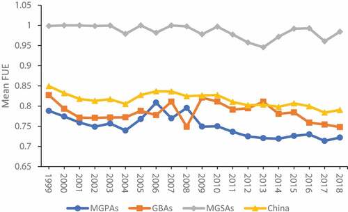
Figure 2. The kernel density distribution of FUE in MGPAs and GBAs. Notes: FUE = fertilizer utilization efficiency; MGPAs = main grain-producing areas; GBAs = grain balance areas; MGSAs = main grain-selling areas.

Figure 1The kernel density distribution of FUE in MGPAs and GBAs. Notes: FUE = fertilizer utilization efficiency; MGPAs = main grain-producing areas; GBAs = grain balance areas; MGSAs = main grain-selling areas.

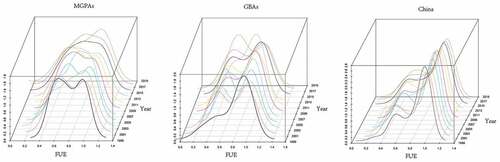
From 1999 to 2018, the nationwide average FUE was 0.8154, reaching a high level. However, there is a significant difference in FUE between the three regions. The mean FUE in MGSAs was 0.9856, 21.87% higher than the national value. The average FUE in MGPAs and GBAs was 0.7499 and 0.7843, 8.01% and 4.82% lower than the national average, respectively. There are multiple peaks in its nuclear density curves in the kernel density map of the whole country (Figure 2). It indicates a polarization phenomenon, meaning an obvious spatial difference in FUE between all the provinces. Moreover, the kernel density curves of MGPAs and GBAs also have multiple peaks. That further indicates remarkable differences in FUE among provinces within the two regions. Therefore, the inequality of FUE hinders the further improvement of national and regional FUE. The contributions of differences within regions and between regions to the total differences will be discussed in detail in the next section.

The FUE in China decreased from 0,8494 to 0.7904 during 1999–2018, presenting a slight fluctuation trend with a decrease of 6.94%. The FUE of MGSAs fluctuated slightly from 1999 to 2010 and was always at or close to 1. The fluctuation was obvious after 2010, and the value reached 0.9457 in 2013, the lowest during the sample period. The FUE of MGPAs fluctuated greatly, presenting a trend of “downward-upward-down” in the whole period. There was a gradual decline from 1999 to 2004, a rapid rise from 2005 to 2008, and a slow decline from 2009 to 2018. MGPAs had the highest FUE in 2006 (0.8086) and 2008 (0.7954), and the lowest FUE in 2017 (0.7136). The FUE of GBAs was the highest in 1999 and 2009 (0.8271 and 0.8209, respectively), and the FUE of GBAs was the lowest in 2008 and 2018 (0.7488 and 0.7480 respectively). The FUE of MGSAs reached the maximum value, 1, in 2000, 2001, 2005, and 2007.

Compared with the other two regions, food production in MGPAs has a significant scale effect. For them, agriculture is an important pillar industry in these provinces with inherent advantages, which can obtain more administrative resources. Therefore, the governments of these provinces pay more attention to introducing and promoting advanced agricultural production technologies and improving the management level of agricultural production organizations. By this logic, MGPAs should have a higher FUE. However, the results show that MGPAs have the lowest FUE, which can be accounted for by the following facts.

First, the provinces belonging to MGPAs are generally backward in economic development and are all inland provinces, except Jiangsu. Economically backward areas often have backward industries and low-income levels of residents. It is difficult for them to attract talent and improve production technology. Second, some provinces have natural endowments unsuitable for agricultural production. Take Inner Mongolia as an example, although it has a large area, it is the province with the largest grassland area, only suitable for animal husbandry, whereas it is not suitable for farming due to cold climate and large areas of desert. With an area of 486,000 square kilometers and a population of 83,700, Sichuan has abundant arable land and agricultural workforces. Nevertheless, Sichuan is primarily mountainous, it is difficult to form large-scale agricultural production mode and agricultural mechanization promotion. Therefore, agricultural production technology in mountainous areas is still very backward. Last but not least, the provinces of the MGPAs are tasked with food production by the central government. With the world’s largest population, China has a great demand for grain and imports grain from abroad every year. China’s national strategy calls for almost self-sufficiency in grain production, much of which needs to be produced by MGPAs’ provinces. That is because other provinces cannot afford significant food production due to several reasons such as insufficient natural resources, extreme weather, or national strategic positioning. It takes more time to improve agricultural production technology and reform agricultural production mode, so it is challenging to meet the requirements of increasing food production tasks and green agricultural production. Under these pressures, they must rely on fertilizers for short-term increases in grain production.

Over the past few decades, China has witnessed a rapid growth in agricultural technology, mechanization level, labor quality, and other aspects. Therefore, China’s agricultural green total factor productivity has been increasing year by year, reflecting a comprehensive performance of the efficiency growth of all factors (Liu & Feng, 2019; D. Liu et al., 2021a; X. Xu et al., 2019). This study shows a gradual decline in FUE, indicating that the efficiency of other factors offset the negative effect of FUE. Fertilizer can increase production and releases agricultural pollution. Therefore, there should be a positive correlation between FUE and environmental efficiency. Although FUE decreased, prior studies showed that the overall environmental efficiency still increased (Huang et al., 2022; Wang & Feng, 2021; Zhang et al., 2019). A possible explanation for this might be that agricultural pollution covered a wide range of areas, and except for the pollution caused by fertilizer, the efficiency of other pollution did improve. Additionally, it can be found that the decline of FUE mainly occurred after 2008, and FUE in China showed a U-shaped trend during 1999–2008. At the end of 2007, the US subprime debt triggered the global financial crisis, which led to many migrant workers’ return to rural areas to engage in agricultural activities, which led to a significant decline in FUE in the following years. Migrant workers return to the countryside to engage in agricultural production and earn a lower income than in cities. They want to produce as much food as possible to get more income. As a result, fertilizer can be used at high intensity as a material that can significantly increase production. Besides, this phenomenon is related to the low prices of fertilizer. The disposable income of Chinese rural residents increased from 2,229 yuan in 1999 to 14,617 yuan in 2018, an increase of 6.5 times, but the price of fertilizers only increased by 1.8 times.⁷

3.2. Spatio-temporal characteristics of FUE at the provincial level

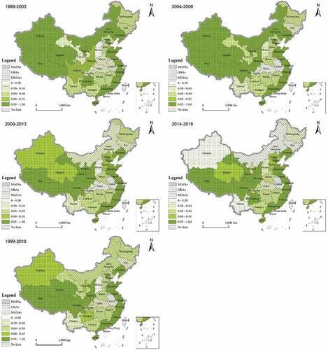
This study divides the whole sample period into four periods (1999–2003, 2004–2008, 2009–2013, 2014–2018), calculated the mean FUE of provinces in each period, and draws the thermal diagrams of four periods and the whole sample period, as shown in Figure Figure 2. During 1999–2003, there were eight provinces with the mean FUE reaching 1, indicating that their FUEs were 1 annually during 1999–2003, meaning that they were all in the production frontier. These provinces include Shanghai, Tibet, Hainan, Beijing, Fujian, Qinghai, Tianjing and Ningxia, six of which are MGSAs. The other two MGSAs, Zhejiang and Gaungdong, also reached 0.9996 and 0.9958, respectively. The lowest province was Shanxi, whose value is 0.3837. Six provinces, including Shanghai, Tibet, Hainan, Beijing, Qinghai and Zhejiang, had a mean FUE of 1 during 2004–2008. The lowest provinces were Anhui (0.4827) and Hubei (0.4774) under the MGPAs. Five provinces were effective DMUs, including Shanghai, Tibet, Hainan, Jiangsu, and Gansu during the period 2009–2013. Among them, Jiangsu belongs to MGPAs. For Shanxi, Anhui, and Hubei, their mean FUEs were below 0.5. Only Gansu and Beijing were efficient DMUs during 2014–2018. There are five areas whose values were lower than 0.5, including Anhui, Xinjiang, Yunnan, Jilin, and Inner Mongolia. During these four periods, the number of provinces with a mean FUE of 1 gradually decreased, while the number of provinces with a mean FUE of less than 0.5 gradually increased, which partially verified the gradual decrease of overall FUE. For the entire sample period, the four provinces with the highest mean FUE were Shanghai (0.9981), Tibet (0.9976), Hainan (0.9975), and Beijing (0.9958), all of which belonged to MGSAs except Tibet. These provinces were efficient DMUs for three of the four periods. In addition, there were 15 provinces with a mean FUE above 0.9, accounting for nearly half of the total. These include all eight MGSAs. The areas with the lowest FUE were Anhui (0.4867) and Shanxi (0.4778).

The economy of Beijing and Shanghai is well developed, both of which are the initial cities promoting advanced technology. The concept of green development has received great attention here. At the same time, the degree of urbanization here is very high, and the agricultural output value only accounts for a small part of the total economic output value. In addition, the huge demand for agricultural products in Beijing and Shanghai has greatly kindled farmers’ enthusiasm for production. Various green technologies can be quickly promoted here, and there is a high FUE here. Hainan has a situation opposite to Beijing and Shanghai. Agriculture occupies a large proportion of the economic output value in Hainan, while the economic level and urbanization rate are low. Due to the large scale of agriculture here, the promotion of green technology will generate great economic benefits. However, other provinces, such as Shandong and Henan with large scale of agriculture, did not obtain high FUE. Hainan is also a tourism-oriented province and attaches great importance to environmental protection. Moreover, its tropical monsoon climate with sufficient rainfall is more suitable for food cultivation. For instance, rice are cultivated three times a year there. The reasons for Tibet’s high FUE are special. Tibet’s climate is unique and complex due to its topography, landform, and atmospheric circulation. It is cold and dry in the northwest and warm and humid in the southeast, not suitable for agricultural production. The organic matter content of most cultivated land is low. Even if a few lands contain more humus, crops seldom absorb them due to low temperature, slow reproduction, small quantity, and slow decomposition of microorganisms. Therefore, the agricultural output value in Tibet accounts for a small proportion, and the intensity and use of the total amount of fertilizer are small.

3.3. Spatial differences and the source decomposition of FUE

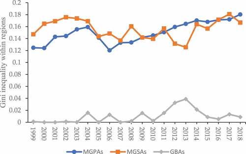
The Gini ratios within the three regions of FUE fluctuated significantly during the sample period, as shown in Figure Figure 3. On the whole, the differences within the three regions showed a widening trend. MGPAs and MGSAs increased from 0.1247 and 0.1471 in 1999 to 0.1803 and 0.1667 in 2018, respectively. It can also be seen in the nuclear density map that there are multiple peaks of the nuclear density curves of MGPAs and GBAs during the sample period. That also suggests that these internal differences were getting bigger. The difference within MGPAs increased before 2004 but decreased sharply during 2004–2006. It reached a minimum of 0.1203 in 2006 (the smallest was in 1999). Its Gini ratio within region rose slowly since 2007. The Gini ratio within MGSAs had a similar trend but fluctuated more violently. The Gini ratio within GBAs was stable before 2004 but fluctuated continuously from 2004 to 2018 and reached the maximum value of 0.0389 in 2013. Its mean in the sample period is 0.0098, much smaller than 0.1501 of MGPAs and 0.1562 of MGSAs. In addition, the Gini ratio within GBAs was smaller than those within MGPAs and MGSAs in every year of the sample period. Before 2009, the Gini ratio within MGSAs was always greater than that within MGPAs, but the situation was just the opposite after 2009.

Figure 3. Provincial distributions of FUE in China in 1999–2003, 2004–2008, 2009–2013, 2014–2018, respectively. Notes: MGPAs = main grain-producing areas; GBAs = grain balance areas; MGSAs = main grain-selling areas.

For the inter-regional differences, the three Gini ratios between regions of FUE showed a significant upward trend, as shown in Figure Figure 4, but there was also regional heterogeneity. Specifically, the inter-regional Gini ratio of MGPAS-GBAS was the highest in the whole sample period, with an average of 0.1588. In general, with the mean values of 0.1406 and 0.1333 in the sample period, the inter-regional Gini ratios of MGPAS-MGSAS and MGSAs-GBAs had little difference. However, before 2009, the inter-regional Gini ratio of MGSAs-GBAs was slightly higher than that of MGPAS-MGSAS. From 2010 to 2018, the inter-regional Gini ratio of MGPAs-MGSAs was higher than that of MGSAs-GBAs. The three Gini ratios between regions have similar fluctuation for the timeline. In addition, this fluctuation is like that of Gini ratios within regions. Those ratios increase gradually in the early stage of the sample period, decline for several years since 2004, and slowly rise after the fluctuation. During the sample period, the inter-regional Gini ratio of MGSAs-GBAs increased the most among the three ratios, increasing from 0.1049 in 1999 to 0.1582 in 2018. The second was that of MGPAs-MGSAs, which increased from 0.1183 to 0.1565, up about 32%; MGPAs-GBAs rose from 0.1445 to 0.1777, an increase of about 23%. The differences between the three functional areas for grain production are significant, and the differences are rising in the fluctuation during the sample period.

Figure 4. The Gini ratios within the three regions during 1999–2018. Notes: MGPAs = main grain-producing areas; GBAs = grain balance areas; MGSAs = main grain-selling areas.

The total difference is decomposed into three parts: the intra-regional difference, the net inter-regional difference and the inter-regional intensity of transvariation. The absolute value and share of each part are reported in Figure Figure 5 and Figure 6. The total difference fluctuated significantly over the sample period and went from 0.1173 in 1999 to 0.1546 in 2018, an 31.8% increase. It can also be seen in the nuclear density map that the peak of the kernel density curve across the country widened during the sample period. The total difference and the difference within MGPAs fluctuated similarly, both showing an increase before 2005, a sharp decline during 2005–2006, and a continued slow rise after 2007. The intra-regional Gini ratio of FUE in China was 0.035 in 1999 and showed an increase before 2004. It decreased between 2004 and 2008, then increased since 2008, and finally rose to 0.0456 in 2018. However, as the total difference increased too fast, its contribution rate declined from 29.86% in 1999 to 29.48% in 2018, and the average contribution rate during the sample period was 29.5%.

Figure 5. The Gini ratios between the three regions during 1999–2018. Notes: MGPAs = main grain-producing areas; GBAs = grain balance areas; MGSAs = main grain-selling areas.

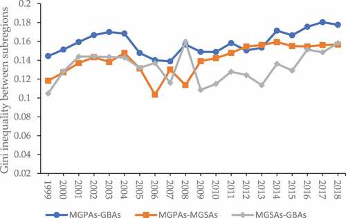
Figure 6. The sources of the total Gini ratios of FUE in China during 1999–2018. Notes: intra-regional difference = ID, net inter-regional difference = NID, inter-regional intensity of transvariation = IID.

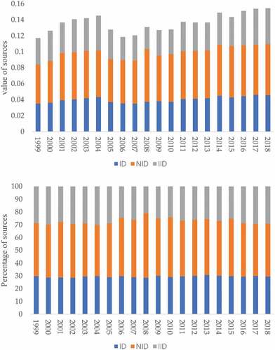
The net difference between regions was 0.0488 in 1999, then gradually increased to 0.0582 in 2004 and decreased to 0.0541 in 2007. In the remaining sample period, the trend of upward fluctuation growth was maintained at 0.0635 in 2018. Its contribution rate to the total difference shows an obvious inverted “U” curve, meaning that it increased from 41.59% in 1999 to 50.38% in 2008 and then slowly decreased to 41.45% in 2018. The average contribution rate during the sample period is 43.4%. In other words, the net difference between regions is the main source of the total difference.

The value and contribution rate of the inter-region intensity of transvariation showed obvious u-shaped characteristics during the sample period. It was 0.0335 in 1999, then gradually decreased to 0.0276 in 2008, and finally rose to 0.0449 in 2018, with the contribution rate ranging from 21.04% to 30.06%. The average contribution rate during the sample period is 27.11%. The inter-region intensity of transvariation reflects the contribution of the overlapping parts of each region to individual differences, and its share in this study is relatively low. It means that China’s classification method of functional grain areas can effectively separate different types of provinces.

The net difference between regions was the primary source of the total difference, and this phenomenon is very normal. The division of agricultural functional areas is based on agricultural production. Behind the differences in agricultural production are differences in various conditions, including geography, climate, population, economic structure, political resources, and historical culture. Differences in these conditions determine differences in FUE. Therefore, the significant regional differences in FUE illustrate the scientific rationality of the Chinese government’s division of agricultural functional areas. This indicator can be used as a reference for the division of agricultural functional areas to adjust the provinces included in each region dynamically. When the government formulates agricultural policies, the positioning of each region must be considered. Therefore, scientific classification of functional areas can lead to better policy performance. The government should focus on narrowing the differences between provinces within a region. The agricultural production conditions of the provinces in a region are similar, so the difference in their FUE should be small. However, the reasons why provinces within a region have high or low FUE are not necessarily exactly the same. For example, Shanghai and Tibet had the high FUEs and belonged to MGSAs. The two provinces are completely different.

4. Conclusions

This study employs the BWMRM to investigate the FUE in China during 1999–2018. In addition, the Kernel Density estimation and Dagum Gini ratio are used to explore its temporal and spatial characteristics.

The main findings can be summarized as follows. First, the FUE of China and the three regions fluctuated slightly downward during the sample period. The mean FUE in MGSAs (0.9856) was the highest, followed by GBAs (0.7843), and then MGPAs (0.7499). Second, there were 15 provinces with a mean FUE above 0.9, including all eight MGSAs. Shanghai (0.9981), Tibet (0.9976), Hainan (0.9975), and Beijing (0.9958) were the top four provinces regarding mean FUEs. The provinces with the lowest mean FUE were Anhui (0.4867) and Shanxi (0.4778). Third, the total difference within China increased by 31.8% over the sample period. The intra-regional contribution, the net inter-regional contribution, and the inter-regional intensity of transvariation accounted for 29.5%, 43.4%, and 27.11% of the total difference. The differences within the three regions had a widening trend during the sample period. The difference within MGSAs was highest before 2009, and that within GBAs was always the lowest among the three regions. For the inter-regional difference, the three Gini ratios between regions of FUE showed a significant upward trend, and the inter-regional difference between MGPAs and GBAs was always the highest.

The findings denote some policy implications. Under the dual pressure of massive demand for food and the goal of achieving carbon neutrality, the Chinese government should vigorously improve the main grain-producing areas ‘s FUE. Grain productions in these areas are high, but FUE is low. Hence, these provinces have great potential, and their FUE is easier to improve than other places. In addition, the government should pay attention to the differences in FUE among provinces within a region rather than the differences between different functional areas. Finally, various policies should be developed following local circumstances, including the local resources and FUE characteristics.

There are some future research recommendations. First, the data used in this study are at the provincial level. China has a vast territory, and a province contains a variety of prefecture-level cities with different geographical environments and climate conditions. Therefore, future studies can use more microscopic data, such as data from prefecture-level cities or counties, to further investigate China’s FUE. Second, future studies can examine the spatial differences of FUE from other regional perspectives. For example, FUE differences between China’s three urban agglomerations (Yangtze River Delta, Guangdong-Hong Kong-Macao Greater Bay Area, and Beijing-Tianjin-Hebei region) can be investigated.

Acknowledgements

This research was funded by Unique Feature and Innovation Project of Guangdong Province (Grant 2021WTSCX092) and the Research Projects of Macao Polytechnic Institute (grant number RP/ESCHS-03/2020 and RP/ESCHS-04/2020).

Disclosure statement

The authors declare that we have no known competing financial interests or personal relationships that could have appeared to influence the work reported in this paper.

Additional information

Funding

This work was supported by the Unique Feature and Innovation Project of Guangdong Province [2021WTSCX092]; the Research Projects of Macao Polytechnic Institute [RP/ESCHS-03/2020]; the Research Projects of Macao Polytechnic Institute [RP/ESCHS-04/2020].

Notes

1. The data comes from: https://data.cnki.net/trade/yearbook/Single/N2021120010?zcode=Z009.

2. In 2008, China’s National Development and Reform Commission released the important policy document the Outline of the National Medium—and long-term Plan for Food Security (2008–2020), which divides China’s 31 provinces into MGPAs, GBAs and MGSAs. http://www.gov.cn/jrzg/2008-11/13/content_1148414.htm.

3. The three yearbooks can be found by the links: https://data.cnki.net/Trade/yearbook/single/N2021120010?zcode=Z009; https://data.cnki.net/yearbook/Single/N2021090092; https://data.cnki.net/yearbook/Single/N2021090054.

4. Rice includes early rice, late rice, in-season rice. Importantly, they have are different carbon emission coefficients in different provinces, due to different geographical climate.

5. Each kind of livestock or poultry has the different breeding cycle, the amount of feeding should be properly adjusted. Average life cycle of pigs, rabbits and poultry are 200 days, 105 days and 55 days respectively. For them, the adjusted formula is $N_i=B{C}_i\times \frac{M_i}{365}$ . $N_i$ is the adjusted quantity, $M_i$ is the quantity before adjustment and $B{C}_i$ is the breeding cycle. For the other livestock and poultry, the adjusted formula is $N_i=\frac{C_{i,t}+C_{i,t-1}}{2}$, $C_{i,t}$ and $C_{i,t-1}$ represent the year-end inventory of years $\mathrm{t}$ and $t-1$, respectively.

6. The FUEs of MGSAs are so concentrated that the kernel density is very high in some values. As a result, their nuclear density curves are very steep and difficult to convey meaningful information. Therefore, this study omitted their graph.

7. The data comes from China Statistical Yearbook and China Year Book of Household Survey.

References

- Aigner, D., Lovell, C. A. K., & Schmidt, P. (1977). Formulation and estimation of stochastic frontier production function models. Journal of Econometrics, 6(1), 21–19. https://doi.org/10.1016/0304-4076(77)90052-5
- Battese, G. E., & Coelli, T. J. (1995). A model for technical inefficiency effects in a stochastic frontier production function for panel data. Empirical Economics, 20(2), 325–332. https://doi.org/10.1007/BF01205442
- Borozan, D. (2018). Technical and total factor energy efficiency of European regions: A two-stage approach. Energy, 152, 521–532. https://doi.org/10.1016/j.energy.2018.03.159
- Chao, S. L. (2017). Integrating multi-stage data envelopment analysis and a fuzzy analytical hierarchical process to evaluate the efficiency of major global liner shipping companies. Maritime Policy & Management, 44(4), 496–511. https://doi.org/10.1080/03088839.2017.1298863
- Chen, P., Yu, M., Chang, C., Hsu, S., & Managi, S. (2015). Nonradial directional performance measurement with undesirable outputs: An application to OECD and Non-OECD countries. International Journal of Information Technology & Decision Making, 14(3), 481–520. https://doi.org/10.1142/S0219622015500091
- Chukalla, A. D., Reidsma, P., van Vliet, M. T. H., Silva, J. V., van Ittersum, M. K., Jomaa, S., Rode, M., Merbach, I., & van Oel, P. R. (2020). Balancing indicators for sustainable intensification of crop production at field and river basin levels. Science of the Total Environment, 705, 135925. https://doi.org/10.1016/j.scitotenv.2019.135925
- Dagum, C. (1998). A new approach to the decomposition of the gini income inequality ratio. Income Inequality, Poverty, and Economic Welfare, 47–63. https://doi.org/10.1007/978-3-642-51073-1_4
- Fujii, H., Managi, S., & Matousek, R. (2014). Indian bank efficiency and productivity changes with undesirable outputs: A disaggregated approach. Journal of Banking & Finance, 38, 41–50. https://doi.org/10.1016/j.jbankfin.2013.09.022
- Fukuyama, H., & Weber, W. L. (2009). A directional slacks-based measure of technical inefficiency. Socio-Economic Planning Sciences, 43(4), 274–287. https://doi.org/10.1016/j.seps.2008.12.001
- Gabriel, J. L., Alonso-Ayuso, M., García-González, I., Hontoria, C., & Quemada, M. (2016). Nitrogen use efficiency and fertiliser fate in a long-term experiment with winter cover crops. European Journal of Agronomy, 79, 14–22. https://doi.org/10.1016/j.eja.2016.04.015
- Granderson, G. (1997). Parametric analysis of cost inefficiency and the decomposition of productivity growth for regulated firms. Applied Economics, 29(3), 339–348. https://doi.org/10.1080/000368497327119
- Greene, W. (2010). A stochastic frontier model with correction for sample selection. Journal of Productivity Analysis, 34(1), 15–24. https://doi.org/10.1007/s11123-009-0159-1
- Guan, W. W., Wu, K., & Carnes, F. (2016). Modeling spatiotemporal pattern of agriculture-feasible land in China. Transactions in GIS, 20(3), 426–447. https://doi.org/10.1111/tgis.12225
- Guo, H., & Liu, X. (2020). Time-space evolution of China’s agricultural green total factor productivity. Chinese Journal of Management Science, 28(9), 66–75. https://doi.org/10.16381/j.cnki.1003-207x.2020.09.007
- Habib, M. A., & Ljungqvist, A. (2005). Firm value and managerial incentives: A stochastic frontier approach. The Journal of Business, 78(6), 2053–2094. https://doi.org/10.1086/497040
- Hellegers, P., & van Halsema, G. (2021). SDG indicator 6.4.1 “change in water use efficiency over time”: Methodological flaws and suggestions for improvement. Science of the Total Environment, 801. https://doi.org/10.1016/j.scitotenv.2021.149431
- Hoang, V.-N., & Coelli, T. (2011). Measurement of agricultural total factor productivity growth incorporating environmental factors: A nutrients balance approach. Journal of Environmental Economics and Management, 62(3), 462–474. https://doi.org/10.1016/j.jeem.2011.05.009
- Huang, X., Feng, C., Qin, J., Wang, X., & Zhang, T. (2022). Measuring China’s agricultural green total factor productivity and its drivers during 1998–2019. Science of the Total Environment, 829, 154477. https://doi.org/10.3390/ijerph16173105
- Huang, X., Xu, X., Wang, Q., Zhang, L., Gao, X., & Chen, L. (2019). Assessment of agricultural carbon emissions and their spatiotemporal changes in China, 1997–2016. International Journal of Environmental Research and Public Health, 16(17), 3105. https://doi.org/10.3390/ijerph16173105
- Hu, W., & Xiong, Z. X. (2021). Do stringent environmental regulations help improve the total factor carbon productivity? Empirical evidence from China’s industrial sectors. Applied Economics, 53(55), 6398–6411. https://doi.org/10.1080/00036846.2021.1940083
- Kumbhakar, S. C., Denny, M., & Fuss, M. (2000). Estimation and decomposition of productivity change when production is not efficient: A paneldata approach. Econometric Reviews, 19(4), 312–320. https://doi.org/10.1080/07474930008800481
- Land, K. C., Lovell, C. A. K., & Thore, S. (1993). Chance-constrained data envelopment analysis. Managerial and Decision Economics, 14(6), 541–554. https://doi.org/10.1002/mde.4090140607
- Lim, D.-J. (2016). Inverse DEA with frontier changes for new product target setting. European Journal of Operational Research, 254(2), 510–516. https://doi.org/10.1016/j.ejor.2016.03.059
- Lin, B. Q., & Tan, R. P. (2016). Ecological total-factor energy efficiency of China’s energy intensive industries. Ecological Indicators, 70, 480–497. https://doi.org/10.1016/j.ecolind.2016.06.026
- Liu, Y., & Feng, C. (2019). What drives the fluctuations of “green” productivity in China’s agricultural sector? A weighted Russell directional distance approach. Resources, Conservation and Recycling, 147, 201–213. https://doi.org/10.1016/j.resconrec.2019.04.013
- Liu, H., Sun, S., & Li, C. (2019). Regional difference and dynamic evolution of fertilizer use efficiency in China under environmental constraints. Issues in Agricultural Economy, 8, 65–75. https://d.wanfangdata.com.cn/periodical/ChlQZXJpb2RpY2FsQ0hJTmV3UzIwMjExMTE2Eg9ueWpqd3QyMDE5MDgwMDgaCDR1OGRlMmR4
- Liu, J. X., Wang, H., Rahman, S., & Sriboonchitta, S. (2021b). Energy efficiency, energy conservation and determinants in the agricultural sector in emerging economies. Agriculture-Basel, 11(8). https://doi.org/10.3390/agriculture11080773
- Liu, G., Wang, B., & Zhang, N. (2016). A coin has two sides: Which one is driving China’s green TFP growth? Economic Systems, 40(3), 481–498. https://doi.org/10.1016/j.ecosys.2015.12.004
- Liu, D., Zhu, X., & Wang, Y. (2021a). China’s agricultural green total factor productivity based on carbon emission: An analysis of evolution trend and influencing factors. Journal of Cleaner Production, 278, 123692. https://doi.org/10.1016/j.jclepro.2020.123692
- Li, W. W., Wang, W. P., Wang, Y., & Ali, M. (2018). Historical growth in total factor carbon productivity of the Chinese industry - A comprehensive analysis. Journal of Cleaner Production, 170, 471–485. https://doi.org/10.1016/j.ecosys.2015.12.004
- Long, X. L., Luo, Y. S., Sun, H. P., & Tian, G. (2018). Fertilizer using intensity and environmental efficiency for China’s agriculture sector from 1997 to 2014. Natural Hazards, 92(3), 1573–1591. https://doi.org/10.1007/s11069-018-3265-4
- Losa, E. T., Arjomandi, A., Dakpo, K. H., & Bloomfield, J. (2020). Efficiency comparison of airline groups in annex 1 and non-annex 1 countries: A dynamic network DEA approach. Transport Policy, 99, 163–174. https://doi.org/10.1016/j.tranpol.2020.08.013
- Nishimizu, M., & Page, J. M. (1982). Total factor productivity growth, technological progress and technical efficiency change: Dimensions of productivity change in Yugoslavia, 1965-78. The Economic Journal, 92(368), 920–936. https://doi.org/10.2307/2232675
- Ohene-Asare, K., Tetteh, E. N., & Asuah, E. L. (2020). Total factor energy efficiency and economic development in Africa. Energy Efficiency, 13(6), 1177–1194. https://doi.org/10.1007/s12053-020-09877-1
- Pastor, J. T., Asmild, M., & Lovell, C. A. K. (2011). The biennial Malmquist productivity change index. Socio-Economic Planning Sciences, 45(1), 10–15. https://doi.org/10.1016/j.seps.2010.09.001
- Pronger, J., Campbell, D. I., Clearwater, M. J., Mudge, P. L., Rutledge, S., Wall, A. M., & Schipper, L. A. (2019). Toward optimisation of water use efficiency in dryland pastures using carbon isotope discrimination as a tool to select plant species mixtures. Science of the Total Environment, 665, 698–708. https://doi.org/10.1016/j.scitotenv.2019.02.014
- Quah, D. (1993). Galton’s fallacy and tests of the convergence hypothesis. The Scandinavian Journal of Economics, 95(4), 427–443. https://doi.org/10.2307/3440905
- Rebolledo-Leiva, R., Angulo-Meza, L., Iriarte, A., & Gonzalez-Araya, M. C. (2017). Joint carbon footprint assessment and data envelopment analysis for the reduction of greenhouse gas emissions in agriculture production. Science of the Total Environment, 593, 36–46. https://doi.org/10.1016/j.scitotenv.2017.03.147
- Ren, Y. J., Peng, Y. L., Campos, B. C., & Li, H. J. (2021). The effect of contract farming on the environmentally sustainable production of rice in China. SUSTAINABLE PRODUCTION AND CONSUMPTION, 28, 1381–1395. https://doi.org/10.1016/j.spc.2021.08.011
- Shestalova, V. (2003). Sequential malmquist indices of productivity growth: An application to OECD industrial activities. Journal of Productivity Analysis, 19(2), 211–226. https://doi.org/10.1023/A:1022857501478
- Wang, R., & Feng, Y. (2021). Research on China’s agricultural carbon emission efficiency evaluation and regional differentiation based on DEA and Theil models. International Journal of Environmental Science and Technology, 18(6), 1453–1464. https://doi.org/10.1007/s13762-020-02903-w
- Wang, Y. B., Shi, L. J., Zhang, H. J., & Sun, S. K. (2017). A data envelopment analysis of agricultural technical efficiency of Northwest Arid Areas in China. Frontiers of Agricultural Science and Engineering, 4(2), 195–207. https://doi.org/10.15302/j-fase-2017153
- Wu, G., Baležentis, T., Sun, C., & Xu, S. (2019). Source control or end-of-pipe control: Mitigating air pollution at the regional level from the perspective of the total factor productivity change decomposition. Energy Policy, 129, 1227–1239. https://doi.org/10.1016/j.enpol.2019.03.032
- Wu, G. Y., Riaz, N., & Dong, R. (2022). China’s agricultural ecological efficiency and spatial spillover effect. Environment Development and Sustainability. https://doi.org/10.1016/j.enpol.2019.03.032
- Xu, X., Huang, X., Huang, J., Gao, X., & Chen, L. (2019). Spatial-temporal characteristics of agriculture green total factor productivity in China, 1998–2016: Based on more sophisticated calculations of carbon emissions. International Journal of Environmental Research and Public Health, 16(20), 3932. https://doi.org/10.3390/ijerph16203932
- Xu, X. C., Wang, Q. Q., & Li, C. (2022a). The impact of dependency burden on urban household health expenditure and its regional heterogeneity in China: Based on quantile regression method. Frontiers in Public Health, 10. https://doi.org/10.3389/fpubh.2022.876088
- Xu, X. C., Yang, H. R., & Li, C. (2022b). Theoretical model and actual characteristics of air pollution affecting health cost: A review. International Journal of Environmental Research and Public Health, 19(6). https://doi.org/10.3390/ijerph19063532
- Yadav, R. L. (2003). Assessing on-farm efficiency and economics of fertilizer N, P and K in rice wheat systems of India. Field Crops Research, 81(1), 39–51. https://doi.org/10.1016/S0378-4290(02)00198-3
- Yang, J. H., & Lin, Y. B. (2020). Driving factors of total-factor substitution efficiency of chemical fertilizer input and related environmental regulation policy: A case study of Zhejiang Province. Environmental Pollution, 263. https://doi.org/10.1016/j.envpol.2020.114541
- Yang, J., Wang, H., Jin, S. Q., Chen, K., Riedinger, J., & Peng, C. (2016a). Migration, local off-farm employment, and agricultural production efficiency: Evidence from China. Journal of Productivity Analysis, 45(3), 247–259. https://doi.org/10.1007/s11123-015-0464-9
- Yang, Y., Wang, S., & Wang, H. (2016b). Evaluation of maize production environmental efficiency based on dynamic DEA in Northeast China. Journal of Agrotechnical Economics, 08, 58–71. https://kns.cnki.net/kcms/detail/detail.aspx?dbcode=CJFD&dbname=CJFDLAST2016&filename=NYJS201608006&v=MjkyOTQ5RllvUjhlWDFMdXhZUzdEaDFUM3FUcldNMUZyQ1VSN2lmWXVkdkZpSGdWYnJMS3pUQmZiRzRIOWZNcDQ=
- Yaqubi, M., Shahraki, J., & Sabouni, M. S. (2016). On dealing with the pollution costs in agriculture: A case study of paddy fields. Science of the Total Environment, 556, 310–318. https://doi.org/10.1016/j.scitotenv.2016.02.193
- Zhang, N., Zhang, G. L., & Li, Y. (2019). Does major agriculture production zone have higher carbon efficiency and abatement cost under climate change mitigation? Ecological Indicators, 105, 376–385. https://doi.org/10.1016/j.ecolind.2017.12.015
- Zhang, S., Zhang, H., Zhang, Z., & Liu, Y. (2022). Evaluation and policy prospect of zero growth action of chemical fertilizer in the 13th five-year plan. Environmental Protection, 50, 31–36. https://kns.cnki.net/kcms/detail/detail.aspx?dbcode=CJFD&dbname=CJFDLAST2022&filename=HJBU202205004&v=MTcxMDBMU2ZKZTdHNEhOUE1xbzlGWUlSOGVYMUx1eFlTN0RoMVQzcVRyV00xRnJDVVI3aWZZdVptRnlqaFVickI=
- Zhang, N., Zhou, P., & Choi, Y. (2013). Energy efficiency, CO2 emission performance and technology gaps in fossil fuel electricity generation in Korea: A meta-frontier non-radial directional distance functionanalysis. Energy Policy, 56, 653–662. https://doi.org/10.1016/j.enpol.2013.01.033
- Zheng, J. F., Gan, P. D., Ji, F., He, D. X., & Yang, P. (2021). Growth and energy use efficiency of grafted tomato transplants as affected by LED light quality and photon flux density. Agriculture-Basel, 11(9). https://doi.org/10.3390/agriculture11090816