A Fundamental Misunderstanding of Risk: The Bias Associated with the Annualized Calculation of Standard Deviation

Abstract

Quantifiable, measurable risk is of critical importance when making data-driven decisions in finance and investment management, but what if the generally accepted practice of the investment industry for calculating risk possessed incorrect mathematical assumptions and embedded biases? This piece revisits the discussion surrounding the methodology used to calculate annualized standard deviation statistics commonly used when reporting the performance of investment products. It goes on to present a new example illustrating the bias when applied to an efficient frontier.

Keywords:

• Risk
• volatility
• investment performance
• bias
• efficient frontier
• standard deviation

PUBLIC INTEREST STATEMENT

Failing to properly understand the inherent risks associated with investment options is serious yet common problem afflicting the world of finance and investing today. Risk in financial markets can manifest itself in many ways ranging from failing to appreciate the terms and conditions of a complex derivative product, underestimating the likelihood of “low probability” events or incorrectly calculating the volatility of a financial instrument. This paper addresses the third issue and aims to illustrate how the investment industry at large is calculating the most commonly-accepted industry measure of volatility and risk in a biased manner that is detrimental to investors.

1. Introduction

Risk lies at the heart of modern finance and investing. Within this world, risk comes from not knowing what the future holds for the performance of financial instruments, and therefore a great deal of effort has been dedicated to developing methods to quantify it. When a wide range of outcomes are possible, the likelihood of negative outcomes increases, which is the reason for expressing financial risk in terms of volatility, such as standard deviation or probability of negative outcome as determined by models based on volatility measures like Value at Risk (VaR). Uncertainty is very important in pricing models. Investors will only invest in bonds that are priced in a manner to compensate investors for the possibility of the bond defaulting, and the seminal Black-Scholes formula for pricing options uses standard deviation to account for market volatility. Investment portfolio decisions are largely based on balancing return against risk, and more specifically, volatility measures. Markowitz (1952) introduced a ground-breaking approach for constructing portfolios by determining the proportional combination of assets that produced the lowest level of risk (in terms of standard deviation) for various levels of portfolio return (Markowitz, 1952). Sharpe (1966) presented a measure for evaluating the performance of portfolios called the “reward-to-variability ratio” that has since become known as the Sharpe Ratio, the proportion of return in excess of the risk-free option expected per unit of risk (standard deviation) (Sharpe, 1966).

The essential role that risk plays in finance is undeniable; however, the manner by which to quantify and represent this risk has been the subject of much research and debate because the consequences of failing to accurately represent the amount of risk in a particular scenario can be dire. Returns are most commonly represented by Gaussian distributions and discussed in terms of means and standard deviations. Many researchers have taken issue with this practice, such as Mandelbrot (1963) who wrote that models based on such distributions misrepresented the likelihood of events in the “fat tails” that represent the most significant outcomes.

But what if there is a misunderstanding of the level of risk at even a more basic level? What if the value that is most commonly used as a measure of risk and uncertainty is being misrepresented?

2. Explanation

Consider how a series of periodic returns translates into the aggregate return represented on a timescale with which people can relate, or more specifically how a series of monthly returns can be expressed as the annual performance.¹ Let $r_i$ represent the percentage change at time $i$ in the price of a financial instrument, $p_i$, calculated by the equation

(1) $r_i=\frac{p_i}{p_{i-1}}-1$(1)

The cumulative performance after period $i$, denoted as $R_i$, is the product of two factors: the return in period $i$, $r_i$, and the cumulative return accumulated prior to $i$ represented as $R_{i-1}$.

(2) $R_i=(1+R_{i-1})(1+r_i)-1$(2)

(3) $R_a=(1+r_1)(1+r_2)\dots (1+r_n)-1$(3)

If this expression was to be simplified where $\bar{r}$ represents the expected monthly return during the $n$ periods of interest. Note that the $\bar{r}$ is calculated using the geometric mean and not the arithmetic. The choice of means was made because the geometric variant accounts for the compounding effect observed in investment returns.

(4) $R_a=\prod _{i=1}^n(1+r_i)-1$(4)

(5) $\bar{r}=\sqrt[n]{R_a+1}-1$(5)

(6) $R_a=(\bar{r}+1{)}^n-1$(6)

Using the expected monthly return result from Equation (5)(5) $\bar{r}=\sqrt[n]{R_a+1}-1$(5) , the standard deviation on a monthly basis, ${\sigma }_M$, can be calculated by

(7) ${\sigma }_M=\sqrt{\frac{1}{n}\sum _{i=1}^n{(r_i-\bar{r})}^2}$(7)

Knowing that the variance of any random variance can be represented as the second moment about the mean, and the standard deviation is the square root of this second moment then the standard deviation of any random variable can be expressed as

(8) $S[X]=\sqrt{E[X^2]-E{[X]}^2}$(8)

Combining the aggregate return calculations from Equation (6)(6) $R_a=(\bar{r}+1{)}^n-1$(6) with Equation (8)(8) $S[X]=\sqrt{E[X^2]-E{[X]}^2}$(8) , an expression for the annualized standard deviation of returns is created

(9) ${\sigma }_A=S[R_a]=\sqrt{E[R_a^2]-E{[R_a]}^2}=S[R_a+1]=\sqrt{E[{(R_a+1)}^2]-E{[R_a+1]}^2}=\sqrt{{({\sigma }_M^2+{(1+\bar{r})}^2)}^n-{(1+\bar{r})}^{(2n)}}$(9)

This is the same result derived in a 1965 article by Tobin (1965)² and has been applied on occasion in academic and professional literature. One such example is Levy and Gunthorpe (1993); however, this approach has failed to be universally accepted as the methodology for making the rather common and extremely critical calculation within the financial world. Kaplan presented the problem and also derives the formula shown in Equation (9)(9) ${\sigma }_A=S[R_a]=\sqrt{E[R_a^2]-E{[R_a]}^2}=S[R_a+1]=\sqrt{E[{(R_a+1)}^2]-E{[R_a+1]}^2}=\sqrt{{({\sigma }_M^2+{(1+\bar{r})}^2)}^n-{(1+\bar{r})}^{(2n)}}$(9) (Kaplan, 2012, 2013). Many academic publications, such as (Craig MacKinlay & Pastor, 2000) and (Lustig et al., 2011), have chosen to use an alternative methodology that introduces a bias into the derived annual value. The commonly-used, alternative method is a function of only the period standard deviation and the level of granularity but not the expected return. As such, this method assumes a linear relationship between, in the case of this example, the monthly and annual standard deviation in which the monthly value is multiplied by the square root of 12,³ the number of periods in a year, as shown in Equation (10)(10) ${\sigma }_A=\sqrt{n}\ast {\sigma }_M$(10) .

(10) ${\sigma }_A=\sqrt{n}\ast {\sigma }_M$(10)

This linear approach shown in Equation (10)(10) ${\sigma }_A=\sqrt{n}\ast {\sigma }_M$(10) has its foundations in basic probability theory. Consider a series of identical, independent (i.i.d.) outcomes, $X_i$, that represent incremental measures of performance within a larger period. The cumulative performance for the entire period, $Y$, can be expressed as the summation of all the $n$ incremental measurements

(11) $Y=\sum _{i=1}^n{X}_i$(11)

Basic axioms of probability show that the relationship between the standard deviations of the random variables $X$ and $Y$ is linear according to

(12) $S[Y]=\sqrt{n}\ast S[X]$(12)

The rationale described in Equations (11(11) $Y=\sum _{i=1}^n{X}_i$(11) ) and (12(12) $S[Y]=\sqrt{n}\ast S[X]$(12) ) is correct and represents mathematical fact when applied to a collection of random variables the cumulative total of which is the sum of all variables in the series; however, it cannot be extended to a series of investment returns. The reason for this is that the cumulative return of an investment security is the result of a compounding, geometric series of returns as described in Equation (4)(4) $R_a=\prod _{i=1}^n(1+r_i)-1$(4) and not the summation of returns. Equation (11)(11) $Y=\sum _{i=1}^n{X}_i$(11) would hold true for the cumulative returns of an investment product if the returns were converted to a logarithmic scale. Unfortunately, many investors do not understand the underlying reasoning for this, which causes them to either over-estimate or under-estimate the level of risk assumed. does not hold for higher order moments, such as standard deviation, so Equation (12)(12) $S[Y]=\sqrt{n}\ast S[X]$(12) cannot be adapted to investment returns by converting returns to a logarithmic scale.

To illustrate the bias that comes with the linear method from Equation (10)(10) ${\sigma }_A=\sqrt{n}\ast {\sigma }_M$(10) review the following example which utilizes the idea of the efficient frontier from Markowitz’s Modern Portfolio Theory (MPT). A theoretical, Pareto optimal frontier is presented in Table 1 showing the minimum amount of risk at each level of portfolio return. The monthly frontier is then converting into the more interpretable annualized form using both of the conversion methods discussed and displayed in Figure 1(a). The difference between the methods, which is the bias referenced throughout this article, is shown in Figure 1(b).

Figure 1. Bias in annual conversion methods

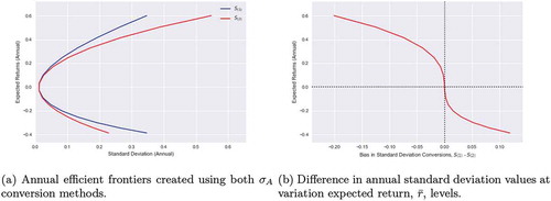
Table 1. Comparison of annual standard deviation values using two methods and the associated bias

Monthly		Annual^4
$\overline{\text{bi}r}$	$\text{bi}{\sigma }_M$	$\text{bi}R$	$\text{bi}{S}_{(1)}$	$\text{bi}{S}_{(2)}$	$\mathbf{\Delta }(S)$
−0.040	0.100	−0.387	0.346	0.227	0.118
−0.034	0.075	−0.345	0.262	0.181	0.081
−0.029	0.055	−0.300	0.191	0.138	0.052
−0.024	0.037	−0.252	0.131	0.101	0.030
−0.018	0.024	−0.202	0.083	0.068	0.015
−0.013	0.013	−0.148	0.047	0.041	0.006
−0.008	0.006	−0.091	0.023	0.021	0.002
−0.002	0.003	−0.031	0.011	0.011	0.000
0.002	0.003	0.032	0.011	0.012	−0.001
0.008	0.006	0.100	0.023	0.026	−0.002
0.013	0.013	0.172	0.047	0.055	−0.007
0.018	0.024	0.248	0.083	0.102	−0.019
0.024	0.037	0.329	0.131	0.171	−0.039
0.029	0.055	0.414	0.191	0.264	−0.073
0.034	0.075	0.505	0.262	0.388	−0.125
0.040	0.100	0.601	0.346	0.547	−0.200

Figure 1(b) shows that the bias is greatest when the expected periodic returns are highest thereby underestimating the amount of risk in a portfolio and fueling the complacency inherent during bullish growth periods in the markets. Conversely, the bias is lowest when the expected returns are lowest during bearish markets causing investors to overestimate the level of volatility and risk in the markets.

The effects of the bias increase as the granularity becomes finer, such as going from monthly data in which there are 12 observation periods per year to daily data with 255 observations per annum. The effects become particularly noticeable for periods of high-expected returns. See the efficient frontier created using daily data in Figure 2(a).

Figure 2. Issues can arise when converting from daily values

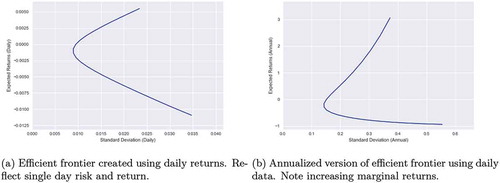
When this frontier is converted to annual version as shown in Figure 2(b), an interesting phenomenon occurs—at the inflection point, the frontier begins to grow instead of decay exponentially. An efficient frontier should exhibit diminishing marginal returns per unit of risk. This result means that an investor must assume increasingly more risk to achieve an additional unit of expected return. The annual efficient frontier in Figure 2(b) shows the opposite effect. This outcome suggests that there exists a point beyond which more expected returns can be achieved by assuming less potential risk. The relationship between risk and return becomes skewed in the transformation process because returns increases exponentially while risk increases linearly. An investor who elects to behave rationally would continue to move further along the exponentially increasing frontier indefinitely because the risk-return profile of the position would continue to improve. Such a representation of the relationship between expected return and risk misrepresents the balance between these two factors and could lead investors into imprudent investment decisions.

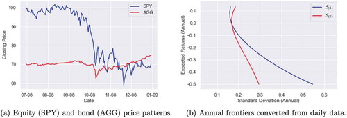
Consider another example from the second half (Q3 and Q4) of 2008 when equity prices (SPY)⁵ were declining rapidly and bond prices (AGG)⁶ were advancing in response to investors exiting the equities market for the bond market as shown in Figure 3(a). If an investor were to use daily closing price data from this two-quarter period to create a frontier on which to base investment decisions and then convert this frontier to annual values, the transformation method produces drastically different levels of portfolio risk. In this declining market, the $S_{(1)}$ transformation (Equation (12))(12) $S[Y]=\sqrt{n}\ast S[X]$(12) fails to consider the impact of negative returns and consequently the reduction in underlying capital, which causes an overestimation of the level of risk. For a portfolio with an expected return of -50%, $S_{(1)}$ estimates standard deviation to be 0.55 compared to the $S_{(2)}$ estimate of 0.29 as illustrated in Figure 3(b). Applying $S_{(1)}$ to a risk conversion instead of $S_{(2)}$ would lead an investor to believe that a portfolio possessed 85% more risk. This belief would make it more difficult for investors to assume more risk in the equity markets in Q1 2009, which marked the end of the so-called Great Recession and a profitable market entry point.

Figure 3. Effect in declining equity market. Example from 2008 (Q3–Q4) on a two asset stock and bond portfolio

3. Conclusion

The topic presented here is not a new arrival in the world of finance. Tobin first presented it in 1965, subsequent white papers in 2012 and 2013 revisited the topic, and financial information provider MorningStar even used it for a period before reverting to the linear method (Standard deviation and sharpe ratio: Morningstar methodology paper, 2005). The objective of this paper is not to introduce a ground-breaking piece of original research but rather to reiterate the need for understanding the way risk is quantified in terms of the volatility of assets and portfolios.

The various techniques used for calculating risk can perceive different levels of risk which in turn can impact the criteria by which decisions are made. This paper elects to use the risk-return characteristics of an investment portfolio as an illustrative example. The relationship between risk and return determine the “optimal” portfolio on an investment frontier, which in turn determines the asset allocation choices for the portfolio. What is of concern more so than two approaches for calculating the same measure of risk arriving at different values is the circumstances under which these approaches differ most. The commonly-used linear method for calculating risk has its greatest negative bias relative to the quadratic approach when returns are high consequently underestimating the level of risk. Such a situation would exist near market peaks after a period of prolonged investment advances thereby making an investor less likely to exit the market. Conversely, the linear conversion method exhibits its greatest positive bias when returns are low, such as at a market bottom. Overestimating the level of risk in a portfolio would make it more difficult for an investor to reenter the market after periods of price decline believing that there exist more volatility and risk. The consequence of not acting or not acting quickly is that investors are slow to assume investment risk and forego favourable buying opportunities.

Investors who make decisions based on statistical measures need to understand the differences in the two methods presented in this paper and the circumstances under which they differ most. Understanding the distinctions can make investors more informed decision makers.

Additional information

Funding

The authors received no direct funding for this research.

Notes on contributors

Matthew W. Burkett

Matthew W. Burkett, Ph.D., is a Senior Director at Ankura Consulting and was a member of Financial Decision Engineering (FDE) research group while completing his Ph.D. at the University of Virginia in the Department of Systems Engineering and Environment where he collaboated with William T. Scherer, Ph.D., on research efforts ranging from agent-based simulations of financial markets, market micro-structure and portfolio decision theory and design.

William T. Scherer

William T. Scherer, Ph.D., is a professor of Systems Engineering in the Department of Systems Engineering and Environment, Associate Chair and Director of the Accelerated Master’s Program (Systems Engineering) at the University of Virginia.

Notes

1. Monthly returns were selected as the granular level for the periodic returns because it is a commonly used practice although the principle being discussed is applicable to more granular data, such as weekly or daily.

2. James Tobin was an American economist who developed the foundational elements of Keynesian economics, served on the Board of Governors of the Federal Reserve System, and taught at Harvard and Yale University. He received the Nobel Memorial Prize in Economic Sciences in 1981 “for his analysis of financial markets and their relations to expenditure decisions, employment, production and prices” (The sveriges riksbank prize in economic sciences in memory of alfred nobel 1981).

3. The level of granularity is represented by the number of periods, $n$, in a year, e.g. 12 months, 52 weeks, and 255 days (average number of trading days in a year).

4. $S_{(1)}$ is the linear transformation method, $S=\sqrt{n}\ast s_n$. $S_{(2)}$ represents the method described in this article, which incorporates $r$ in the calculation to created an annualized figure.

5. SPDR S&P 500 ETF, which replicates the S&P 500 and serves as a surrogate for the US stock market.

6. iShares Core U.S. Aggregate Bond ETF, which acts as a representation of the aggregate US bond market.

References

- Craig MacKinlay, A., & Pastor, L. (2000). Asset pricing models: Implications for expected returns and portfolio selection. The Review of Financial Studies, 13(4), 883. https://doi.org/10.1093/rfs/13.4.883
- Kaplan, P. D. (2012). What’s wrong with multiplying by the square root of twelve. Journal of Performance Measurement, 17(2), 16–7. https://spauldinggrp.com/product/whats-wrong-multiplying-square-root-twelve/
- Kaplan, P. D. (2013, January). What’s wrong with multiplying by the square root of twelve (Technical Report). Morningstar.
- Levy, H., & Gunthorpe, D. (1993). Optimal investment proportions in senior securities and equities under alternative holding periods. The Journal of Portfolio Management, 19(4), 30–36. https://doi.org/10.3905/jpm.1993.409457
- Lustig, H., Roussanov, N., & Verdelhan, A. (2011). Common risk factors in currency markets. The Review of Financial Studies, 24(11), 3731. https://doi.org/10.1093/rfs/hhr068
- Mandelbrot, B. (1963). The variation of certain speculative prices. The Journal of Business, 36(4), 394–419. https://doi.org/10.1086/jb.1963.36
- Markowitz, H. (1952). Portfolio selection. The Journal of Finance, 7(1), 77–91.
- Sharpe, W. F. (1966). Mutual fund performance. The Journal of Business, 39(1), 119–138. https://doi.org/10.1086/294846
- Standard deviation and sharpe ratio: Morningstar methodology paper. (2005, January). (Technical Report). Morningstar. https://gladmainnew.morningstar.com/directhelp/Methodology_StDev_Sharpe.pdf
- The Royal Swedish Academy of Sciences. (1981, October 13). This year’s prize in economics awarded for research on the financial system and its effects on inflation and employment (Press release). Retrieved from https://www.nobelprize.org/prizes/economic-sciences/1981/press-release/
- Tobin, J. (1965). The theory of portfolio selection. In FH Hahn and FRP Brechling (eds), The Theory of Interest Rate (pp. 3-51). London: Macmillan.