NURBS Enhanced Virtual Element Methods for the Spatial Discretization of the Multigroup Neutron Diffusion Equation on Curvilinear Polygonal Meshes

Abstract

The Continuous Galerkin Virtual Element Method (CG-VEM) is a recent innovation in spatial discretization methods that can solve partial differential equations (PDEs) using polygonal (2D) and polyhedral (3D) meshes. Recently, a new formulation of CG-VEM was introduced which can construct VEM spaces on polygons with curvilinear edges. This paper presents the application of the curved VEM to the multigroup neutron diffusion equation and demonstrates its benefits over the conventional straight-sided VEM for a number of benchmark verification test cases with curvilinear domains. These domains were constructed using a topological data-structure developed as part of this paper, based on the doubly-connected edge list, with curves and surfaces both represented using non-uniform rational B-splines (NURBS). This data-structure is used both to specify the geometry of the reactor and to represent the curvilinear polygonal mesh. We also present two separate methods of performing integrations on curvilinear polygons, one for homogeneous functions and one for non-homogeneous functions.

Keywords:

• Virtual element method
• neutron diffusion equation
• polygonal mesh
• NURBS
• high-order mesh

1. Introduction

The multigroup neutron diffusion equation (NDE) is a coupled system of elliptic, second-order partial differential equations (PDEs). It is a special case of the neutron transport equation (NTE), where the angular dependence of the angular flux is linearly anisotropic (Hebert 2020). The NDE is widely used in the nuclear industry for whole-core nuclear reactor analysis simulations (Gaston et al. 2015; Mylonakis et al. 2014). Whole-core simulations are typically the final stage of a nuclear reactor core analysis and are usually performed using coarse mesh nodal methods (Lawrence 1986; Smith 2017; Sanchez 2009; Smith 1986). The nodal reactor analysis simulations utilize spatially homogenized, and energy group condensed, macroscopic neutron cross section data for each of the nuclear fuel assemblies (or nodes) within the reactor core (Lawrence 1986; Smith 2017; Sanchez 2009; Smith 1986). Nuclear reactor lattice physics computations are performed to determine the spatially homogenized and energy group condensed macroscopic neutron cross section data as well as assembly discontinuity factors (ADFs). These nuclear reactor lattice physics codes solve the neutron transport equation for a single nuclear fuel assembly (or node) with prescribed periodic boundary conditions (Lawrence 1986; Smith 2017; Sanchez 2009; Smith 1986). Typically between 2 to 4 energy groups are used when solving the NDE across the whole nuclear reactor core. The whole-core calculation is used to compute quantities such as the power distribution in the nuclear reactor core and nuclear fuel burn-up or depletion (Hebert 2020). This approach to nuclear reactor core analysis has been developed over decades and was initially conceived when computing resources were far less developed. As computing resources have grown over recent decades it has become feasible to perform calculations on nuclear reactor geometries which have not been spatially homogenized, for example see (Stimpson et al. 2020; Collins et al. 2020). This presents an opportunity to produce high-fidelity solutions where spatial information is not lost in the homogenization process, but it also poses an additional challenge. This challenge is to faithfully represent the full set of geometric features of the nuclear reactor within the computational mesh. Early numerical methods, such as the nodal method, were limited to structured, Cartesian grids and were therefore not able to exactly model complex, curvilinear geometric features.

The finite element method (FEM), which was first applied to neutron transport in the 1970s (Semenza, Lewis, and Rossow 1972; Kang and Hansen 1973), was an important advance in improved geometrical modeling capability. For the first time, unstructured meshes could be used to discretise the NTE. Unstructured finite element (FE) meshes are better able to approximate curvilinear geometries than structured Cartesian meshes. The key disadvantage of the FEM was the initial limitation to straight-sided elements, which result in a discrepancy between the computational mesh and the geometric domain. Higher-order isoparametric FEM, which has a piece-wise polynomial description of geometry, are often used to reduce this discrepancy. However, even the high-order isoparametric FEM is unable to exactly represent conic sections in 2D and quadric surfaces in 3D, meaning the mesh-geometry discrepancy is not eliminated. This is of particular relevance to nuclear reactor physics as many reactor designs feature cylindrical fuel rods. For a FEM scheme of higher polynomial order ($p\ge 2$), the geometric discrepancy becomes the dominant source of spatial discretization error relative to the other sources of error, which are the approximation error and the integration error. The approximation error arises due to difference between the approximate solution, which is expanded in a finite-dimensional global FE basis, and the exact solution. While the integration error occurs due to the discrepancy between analytic integrals and integrals performed by numerical quadrature. In this paper, we are primarily concerned with the approximation error and the geometric error. The integration error can always be reduced by increasing the order of quadrature. In fact, it was shown in (Ciarlet 2002) Section 4.1, that for a FEM scheme of order p that numerical quadrature of order $\ge 2(p-1)$ is sufficient to guarantee that numerically integrated bilinear form is still coercive and that the FEM scheme will converge with the expected order of accuracy. A more recent innovation in the finite element method was the advent of the NURBS-enhanced finite element method (NE-FEM) (Sevilla, Fernández-Méndez, and Huerta 2008; Sevilla, Fernández-Méndez, and Huerta 2011), from whom we took inspiration for the name of our own method. In the NE-FEM, the mapping between parent space and real space is constructed using the NURBS definition of the boundary curves. The NE-FEM therefore also eliminates the geometry error between the computational mesh and the geometric domain from the lowest level of mesh refinement. The authors demonstrate that the NE-FEM exhibits optimal order of convergence for problems with curvilinear NURBS boundaries. The NE-FEM is still limited to triangular/quadrilateral meshes in 2D and tetrahedral/hexahedral meshes in 3D however.

Isogeometric analysis (IGA) (Hughes, Cottrell, and Bazilevs 2005) is a spatial discretization method designed to minimize the geometric model error between the computer aided geometric design (CAGD) geometric description of a domain and the computational mesh. It is a weighted-residual (WR) Galerkin spatial discretization where the basis functions used to represent the solution field are the same as those used to describe the geometry, in this case the Non-Uniform Rational B-spline basis, which is ubiquitous in CAGD. NURBS are capable of representing a wide variety of geometries including conic sections in 2D and quadric surfaces in 3D, making them very useful for the analysis of nuclear reactors. IGA has already been applied to numerous areas of nuclear reactor physics including the neutron diffusion equation, the even-parity form of the NTE, the first-order form of the NTE, the self-adjoint angular flux (SAAF) form of the NTE and the weighted least squares (WLS) form of the NTE (Owens et al. 2016; Hall, Eaton, and Williams 2012; Owens, Kópházi, and Eaton 2017a; Owens et al. 2017b; Owens et al. 2017c; Welch et al. 2017a; Welch et al. 2017b; Latimer et al., 2020; Latimer et al., 2020; Latimer et al. 2021). Many of these papers demonstrate a marked improvement in numerical accuracy for a given number of degrees of freedom (DoF) when compared to conventional finite elements of equal polynomial order. However, IGA has one potential disadvantage which is that a piece-wise volumetric NURBS parametrisation of the computational domain is required. Further, this volumetric NURBS parametrisation must be constructed from the representation of geometry found in most commercial CAD software which is the boundary-representation (b-rep). The b-rep is a topological structure which stores the incidence and adjacency of vertices, edges, faces and volumes. Faces, edges and vertices are then mapped to surfaces, curves and points which encode how these entities are embedded in 3D space. The process of producing an analysis-suitable NURBS mesh from a b-rep involves subdividing the computational domain, which may have complicated topology, into individual sub-regions which are curvilinear quadrilaterals in 2D and curvilinear hexahedra in 3D (Hughes, Cottrell, and Bazilevs 2005). Even with the use of hanging-node discontinuous IGA (Owens et al. 2016; Owens, Kópházi, and Eaton 2017a; Owens et al. 2017b; Owens et al. 2017c), constrained node continuous IGA (Latimer et al. 2021) or T-spline IGA methods (Harmel, Sauer, and Bommes 2017; Bazilevs et al. 2010) this represents a significant geometrical challenge. Some approaches to this problem may be found in (Khamayseh and Hamann 1996; Aigner et al. 2009; Xu et al. 2013a; Xu et al. 2013b; Lin et al. 2015; Schneider, Panozzo, and Zhou 2021; Schmidt, Wüchner, and Bletzinger 2012). Therefore, an alternative to IGA would be a method which employs a more conventional notion of mesh, in the sense of finite elements, but is able to preserve the full geometric information of the original geometry. One such numerical method is the virtual element method (VEM).

The virtual element method (VEM) is a generalization of the Galerkin finite element method (FEM) to polytopal grids. The VEM was first introduced in (Beirão da Veiga et al. 2013) for Poisson’s equation, which introduced the canonical H¹-conforming, C⁰-continuous virtual element. Around the same time the H²-conforming, C¹-continuous virtual element method for plate bending problems (Brezzi and Marini 2013) was also introduced. The VEM literature has since expanded substantially from these two original papers. In (da Veiga and Manzini 2014) the VEM was extended to include schemes with arbitrary regularity, i.e. C^m continuous with any m > 0, while in in (Manzini, Cangiani, and Sutton 2014; da Veiga et al. 2016) the H¹-conforming VEM for general second-order elliptic problems was presented. Other major breakthroughs on VEM theory include the development of the computable L² projection (Ahmad et al. 2013), the reduction of internal degrees of freedom (Beirão da Veiga et al. 2016a; Russo 2016), nonconforming discretisations (Antonietti, Manzini, et al. 2018; Cangiani, Manzini, and Sutton 2016; Berrone, Borio, and Manzini 2018; Ayuso de Dios, Lipnikov, and Manzini 2016; Liu, Li, and Chen 2017) and stabilisations and L²-orthogonalised local polynomial bases (Dassi and Mascotto 2018; Mascotto 2018; Berrone and Borio 2017). A rigorous analyses of stability and a priori error estimates may be found in (Brenner, Guan, and Sung 2017; Brenner and Sung 2018; da Veiga, Lovadina, and Russo 2017). Recently, formulations involving H¹ virtual elements with curvilinear edges have been presented (Beirão da Veiga, Russo, and Vacca 2019; Bertoluzza, Pennacchio, and Prada 2019; Beirão da Veiga et al. 2020), with the version presented in (Beirão da Veiga, Russo, and Vacca 2019) being the one that has been used in this paper to solve the Neutron Diffusion Equation (NDE). One of the important advantages of the VEM presented in (Beirão da Veiga, Russo, and Vacca 2019) is its simplicity since an algorithm developed for a straight-sided VEM, such as that in (Beirão da Veiga et al. 2013) can easily be modified to accommodate curvilinear edges.

The novelty presented in this paper is the use of Non-Uniform Rational B-spline geometry, in conjunction with curvilinear VEM of (Beirão da Veiga, Russo, and Vacca 2019), to develop a high-order, exact-geometry discretization of the multigroup neutron diffusion equation (NDE). This is a direct extension of the research we presented in (Ferguson, Kópházi, and Eaton 2021), where it was shown that the geometric error was causing convergence rates in various quantities of interest (QoI) to saturate at second-order, irrespective of the polynomial order of the VEM scheme. This paper demonstrates that such effects can be eliminated using NURBS-enhanced VEM (NE-VEM) algorithms. Eliminating the geometric error means that the benefits of higher order VEM schemes are fully realized and this will be demonstrated through a series of benchmark verification test cases. Additionally, this paper will describe many of the algorithmic details needed to implement a computationally efficient NE-VEM, including a geometry/mesh data structures for both building nuclear reactor geometries and for representing curvilinear polygonal meshes and numerical integration on curvilinear polygons.

This paper is organized as follows: in Section 2 we review the definition of the curvilinear, H¹-conforming virtual element space that has previously been developed within the existing research literature (Beirão da Veiga, Russo, and Vacca 2019). These are the local function spaces which we shall use to discretise the multigroup NDE. In Section 3 we derive the variational form of the multigroup neutron diffusion equation and present the virtual element discretization of both the fixed-source and effective multiplication factor (${\mathrm{K}}_{\text{eff}}$), or k-eigenvalue, nuclear reactor physics problems. In Section 4 we present the data structure we developed to efficiently store both NURBS-based models of nuclear reactor geometries and NURBS-based curvilinear polygonal meshes. We also present the geometric model we developed to represent curvilinear polygons with NURBS edges. In Section 5 we present the method we developed to perform high-order numerical integration of homogeneous functions (in particular the set of monomials up to a given order) and general functions using a NURBS surface tessellation of curvilinear polygons. High-order numerical integration which incorporates exact-geometry information is the key to obtaining the maximum possible accuracy from the high-order VEM on curvilinear meshes. In Section 6 we present three numerical test cases which demonstrate the benefits of using the NE-VEM over standard straight-sided VEM for problems with curvilinear geometry. Finally, in Section 7 we give some concluding remarks.

2. The curved VEM

The theory of the NE-VEM shall be presented in this section. The formulation presented here is taken primarily from the previous research literature in the field (Beirão da Veiga et al. 2013; Ahmad et al. 2013; Russo 2016; Beirão da Veiga et al. 2016b) with the extension to curvilinear domains introduced in (Beirão da Veiga, Russo, and Vacca 2019).

2.1. Preliminaries

Vectors in ${\mathbb{R}}^d$ are denoted with lower case bold e.g. v and the element at index i of a vector is denoted ${(\mathbf{v})}_i.$ Matrices in ${\mathbb{R}}^{m\times n}$ are denoted using upper case bold e.g. A and the element at index (i, j) of a matrix is denoted ${(\mathbf{A})}_{i,j}.$ Given a domain $E\subset {\mathbb{R}}^d$ the diameter, centroid and measure are denoted h_E, ${\mathit{x}}_E$ and $\left|E\right|$ respectively. If E is a polygon then the number of vertices, edges and degrees of freedom present in it are denoted $N_v^E,N_e^E$ and $N_{\text{dof}}^E$ respectively.

Let the domain of interest V be bounded by a set of n general NURBS curves, denoted ${\left\{{\Gamma }_i\right\}}_{i=1}^n,$ with the only restriction being that each curve is a member of C^m, with $m\ge 0.$ We shall let ${\left\{{\mathcal{T}}_h\right\}}_h$ denote a family of partitions of V where h denoted the maximum face diameter in the mesh: $h={\max }_{F\in {\mathcal{T}}_h^{}}{h}_F.$ The mesh shall satisfy the usual restrictions: that faces are non-overlapping and share one or more edges only if they are adjacent. The faces themselves are each bounded polygons with possibly curved edges. The set of faces in the mesh ${\mathcal{F}}_h$ may be split into two disjoint sets: ${\mathcal{F}}_h^i$ and ${\mathcal{F}}_h^b$ such that ${\mathcal{F}}_h={\mathcal{F}}_h^i\cup {\mathcal{F}}_h^b.$ The set ${\mathcal{F}}_h^i$ are the internal faces, defined as the set of faces that are not incident with a geometric curve. 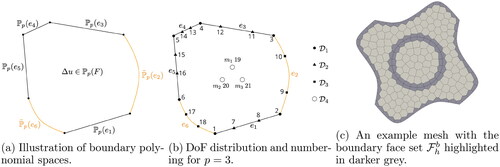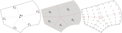The set ${\mathcal{F}}_h^b$ are the boundary faces, defined as those faces which are incident with a geometric curve. An example is presented in Figure 1c. The reason for making the distinction between these two sets of faces is that the faces $F\in {\mathcal{F}}_h^i$ are guaranteed to have all their edges be straight lines. Therefore, the local curved virtual element spaces coincide with classical VEM described in (Beirão da Veiga et al. 2013; Beirão da Veiga et al. 2016b; Beirão da Veiga et al. 2014). The faces $F\in {\mathcal{F}}_h^b$ however, may have one or more of their edges be curvilinear. Therefore, the local curved VEM spaces diverge from the classical ones. Similarly we may split the set of edges in ${\mathcal{T}}_h^{},$ denoted ${\mathcal{E}}_h$ into boundary edges ${\mathcal{E}}_h^b$ and internal edges ${\mathcal{E}}_h^i.$ All edges may either be straight or curvilinear depending on whether they are incident on either curved boundaries or curved internal interfaces. We make the following mesh regularity assumptions:

Figure 1. Illustration of the VEM DoFs on a curvilinear polygon and an example of a curvilinear polygonal mesh (right).

Assumption 2.1.

(Mesh Regularity) The exists a positive constant η such that

• for every face $F\in {\mathcal{T}}_h^{}$ the length of all the edges of F have length $\ge \eta h_F.$

• every face $F\in {\mathcal{T}}_h^{}$ is star-shaped with respect to a ball B_F with radius $\eta h_F.$

We denote the usual norm and seminorm in the Sobolev spaces as ${\Vert v\Vert }_{s,E},{\left|v\right|}_{s,E}$ for all v in $H^s(E)$ and we denote the the the broken Sobolev space and broken polynomial space as: $$H^s({\mathcal{T}}_h^{})=\left\{v\in L^2(V):v{|}_F\in H^s(F)\hspace{1em}\forall F\in {\mathcal{T}}_h^{}\right\},$$ $${\mathbb{P}}_p({\mathcal{T}}_h^{})=\left\{q_p\in L^2(V):q_p{|}_F\in {\mathbb{P}}_p(F)\hspace{1em}\forall F\in {\mathcal{T}}_h^{}\right\}.$$

We define the broken Sobolev norms on $H^s({\mathcal{T}}_h^{})$ in the usual way: $${\Vert v\Vert }_{s,h}={\left(\sum _{F\in {\mathcal{T}}_h^{}}{\Vert v\Vert }_{s,F}^2\right)}^{1/2},\hspace{1em}{\left|v\right|}_{s,h}={\left(\sum _{F\in {\mathcal{T}}_h^{}}{\left|v\right|}_{s,F}^2\right)}^{1/2}.$$

Finally, we define the set of scaled monomials of order $\le p$ on face F as: $${\mathcal{M}}_p(F)=\left\{m_{\alpha }(\mathit{x})={\left(\frac{x-x_F}{h_F}\right)}^{{\alpha }_x}{\left(\frac{y-y_F}{h_F}\right)}^{{\alpha }_y}:{\alpha }_x+{\alpha }_y\le p\right\},$$ and use ${\mathcal{M}}_p(F)$ as a basis for ${\mathbb{P}}_p(F)$ therefore the dimension of ${\mathbb{P}}_p(P)$ is given by: $n_p=(p+1)(p+2)/2.$ Following (Beirão da Veiga et al. 2014) we establish the following ordering between 1D index α and multi-index $({\alpha }_x,{\alpha }_y):$ (2.1) $$1\iff (0,0),\hspace{1em}2\iff (1,0),\hspace{1em}3\iff (0,1),\hspace{1em}4\iff (2,0),\hspace{1em}5\iff (1,1),\hspace{1em}6\iff (0,2),\dots$$(2.1)

This mapping shall be denoted $\alpha (i,j).$

2.2. The local curved VE space

2.2.1. The initial space

Given a curved polygon $F\in {\mathcal{T}}_h^{},$ on each edge e, straight or curved, let ${\gamma }_e:[0,1]\to e$ be the NURBS parametrisation of that edge. The forward mapping is denoted $\mathit{x}={\gamma }_{e}t$ and the inverse mapping $t={\gamma }_e^{-1}\mathit{x}.$ We define a 1D polynomial space ${\mathbb{P}}_p([0,1])$ from which we may define a pseudo-polynomial space on each edge e $${\tilde{\mathbb{P}}}_p(e):=\left\{{\tilde{q}}_p({\gamma }_{e}t)=q_p(t)\hspace{1em}:\hspace{1em}{p}_p\in {\mathbb{P}}_p([0,1])\hspace{1em}\forall t\in [0,1]\right\}.$$

Note ${\tilde{\mathbb{P}}}_p(e)$ will not be polynomial unless γ_e is an affine map. Let F be bounded by the union of a set of curvilinear edges ${\tilde{\mathcal{E}}}_F$ and a set of straight edges ${\mathcal{E}}_F$ such that $\partial F={\tilde{\mathcal{E}}}_F\cup {\mathcal{E}}_F.$ Following the usual process of constructing local VEM spaces for elliptic operators we begin by defining a boundary space $B_p(\partial F):$ $${\mathcal{B}}_p(\partial F):=\left\{v:v\in C^0(\partial F)\hspace{1em}\text{and}\hspace{1em}v{|}_{\tilde{e}}\in {\tilde{\mathbb{P}}}_p(\tilde{e})\hspace{1em}\forall \tilde{e}\in {\tilde{\mathcal{E}}}_F\hspace{1em}\text{and}\hspace{1em}v{|}_e\in {\mathcal{P}}_p(e)\hspace{1em}\forall e\in {\mathcal{E}}_F\right\}.$$

With ${\mathcal{B}}_p(\partial F)$ defined, the initial local VEM space may be constructed as follows: $${\tilde{\mathcal{V}}}_p(F):=\left\{v\in H^1(F):v{|}_{\partial F}\in {\mathcal{B}}_p(\partial F)\hspace{1em}\text{and}\hspace{1em}\Delta v\in {\mathbb{P}}_p(F)\right\}$$

We now present two propositions about the dimension of both ${\mathcal{B}}_p(\partial F)$ and ${\tilde{\mathcal{V}}}_p(F).$

Proposition 2.1.

For a polygon F with $N_e^F$ edges, ${\mathcal{B}}_p(\partial F)$ has dimension $p{N}_e^F$ and ${\tilde{\mathcal{V}}}_p(F)$ has dimension $p{N}_e^F+n_p.$

See ((Beirão da Veiga, Russo, and Vacca 2019), proposition 2.2) and ((Ahmad et al. 2013), proposition 1) for a short proof.

Figure 1a illustrates ${\tilde{\mathcal{V}}}_p(F)$ on an example curved polygon where e₂, e₆ (shown in orange) are curved and the remaining edges are straight. We may define the following linear functionals on ${\tilde{\mathcal{V}}}_p(F)$ (Beirão da Veiga, Russo, and Vacca 2019):

• ${\mathcal{D}}_1:$ The value of v at each of the vertices of F.

• ${\mathcal{D}}_2:$ The value of v at the p – 1 internal points of the p + 1 Gauss-Lobatto quadrature on $e\in {\mathcal{E}}_F.$

• ${\mathcal{D}}_3:$ The value of v at each of the points given by $\mathit{x}={\gamma }_{\tilde{e}}t$ where t is a member of the p – 1 internal points of the p + 1 Gauss-Lobatto rule on $[0,1]$ and ${\gamma }_{\tilde{e}}:[0,1]\to \tilde{e}$ is the NURBS parameterization for curve $\tilde{e}\in {\tilde{\mathcal{E}}}_F.$

• ${\mathcal{D}}_4:$ The moments with the members of ${\mathcal{M}}_{p-2}(F):$ $$\frac{1}{\left|F\right|}\int v{m}_{\alpha }^{}dx\hspace{1em}\forall m_{\alpha }\in {\mathcal{M}}_{p-2}\left(F\right).$$

Using these linear functionals, it is possible to compute three important projection operators: the energy projector ${\Pi }_p^{\nabla }:H^1(F)\to {\mathbb{P}}_p(F),$ the gradient projector ${\Pi }_{p-1}^0\nabla :H^1(F)\to {[{\mathbb{P}}_{p-1}(F)]}^2$ and the $L^2(F)$ projection ${\Pi }_{p-2}^0:L^2(F)\to {\mathbb{P}}_{p-2}(F).$

Definition 2.2.

(The energy projector) The energy projector is defined by the following projection onto constants and the following orthogonality condition: $${\int }_{\partial F}{\Pi }_p^{\nabla }v-\mathit{vdx}=0\hspace{1em}\forall v\in H^1(F)$$ $${\left(\nabla \left({\Pi }_p^{\nabla }v-v\right),\nabla q_p\right)}_{0,F}=0\hspace{1em}\forall v\in H^1(F)\hspace{1em}\text{and}\hspace{1em}\forall q_p\in {\mathbb{P}}_p(F).$$

Definition 2.3.

(The gradient projector) The gradient projector is defined by the following orthogonality condition: $${\left({\Pi }_{p-1}^0\nabla v-\nabla v,{\mathbf{q}}_{p-1}\right)}_{0,F}=0\hspace{1em}\text{for}\hspace{1em}{\mathbf{q}}_{p-1}\in {[{\mathbb{P}}_{p-1}(F)]}^2,$$

Definition 2.4.

(The L² projector) The L² projector is defined by the following orthogonality condition. $${\left({\Pi }_{p-2}^{0}v-v,q_{p-2}\right)}_{0,F}=0\hspace{1em}\forall v\in H^1(F)\hspace{1em}\text{and}\hspace{1em}\forall q_{p-2}\in {\mathbb{P}}_{p-2}(F).$$

2.2.2. The enhanced virtual element space

The initial virtual element space ${\tilde{\mathcal{V}}}_p(F)$ is sufficient to solve pure diffusion problems. However, if one wishes to solve problems involving either convection or reaction terms then the full $L^2(F)$ projector is required. Following the method of (Ahmad et al. 2013), it is possible to construct the enhanced virtual element space in which the full L² projection onto ${\mathbb{P}}_p(F)$ is computable from just the linear functionals ${\mathcal{D}}_1-{\mathcal{D}}_4.$ The enhanced virtual element space is defined as follows $${\mathcal{V}}_p(F):=\left\{v\in {\tilde{\mathcal{V}}}_p(F):{\left(v,q_p\right)}_{0,F}={\left({\Pi }_p^{\nabla }v,q_p\right)}_{0,F}\hspace{1em}\forall q_p\in {\overline{\mathbb{P}}}_p(F)\cup {\overline{\mathbb{P}}}_{p-1}(F)\right\},$$ where ${\overline{\mathbb{P}}}_p(F)={\mathbb{P}}_p(F)/{\mathbb{P}}_{p-1}(F)$ is the set of polynomials of order strictly equal to p. Therefore, ${\mathcal{V}}_p(F)\subset {\tilde{\mathcal{V}}}_p(F),$ and is the set comprised of all functions $v\in {\tilde{\mathcal{V}}}_p(F)$ for which the internal moments of v and ${\Pi }_p^{\nabla }v$ coincide for orders p − 1 and p. The linear functionals ${\mathcal{D}}_1,\dots ,{\mathcal{D}}_4$ are well defined on ${\mathcal{V}}_p(F)$ and may be taken as a set of insolvent degrees of freedom, meaning that every $v\in {\mathcal{V}}_p(F)$ is uniquely determined by the values of ${\mathcal{D}}_1-{\mathcal{D}}_4.$

Proposition 2.5.

For a polygon F with $N_e^F$ edges the dimension of ${\mathcal{V}}_p(F)$ is $p{N}_e^F+n_{p-2}$ and the linear functionals ${\mathcal{D}}_1,\dots ,{\mathcal{D}}_4$ may be taken as a unisolvent set of degrees of freedom.

See ((Ahmad et al. 2013), proposition 2) for a proof. With unisolvence established, the linear functionals ${\mathcal{D}}_1,\dots ,{\mathcal{D}}_4$ shall now be referred to as degrees of freedom (DoFs) and $\mathrm{dim\hspace{0.17em}}{\mathcal{V}}_p(F)$ shall be denoted $N_{\text{dof}}^F.$ The i’th degree of freedom shall be denoted ${\text{dof}}_i(v):{\mathcal{V}}_p(F)\to {\mathbb{R}}^{}$ and the local Lagrangian basis ${\phi }_i\in {\mathcal{V}}_p(F)$ satisfies: $${\text{dof}}_i({\phi }_j)={\delta }_{i,j}\hspace{1em}\text{for}\hspace{1em}i,j=1,\dots ,N_{\text{dof}}^F.$$

Every $v\in {\mathcal{V}}_p(F)$ has a unique representation in the local Lagrangian basis: $$v=\sum _{i=1}^{N_{\text{dof}}^F}{\text{dof}}_i(v){\phi }_i.$$

Remark 1.

Due to the fact the the boundary spaces ${\tilde{\mathbb{P}}}_p(e)$ are not polynomial unless ${\gamma }_e:[0,1]\to e$ is an affine map, then in general the set of polynomials ${\mathbb{P}}_p(F)$ are not contained in ${\mathcal{V}}_p(F)$ (i.e ${\mathbb{P}}_p(F)\cancel{\subset }{\mathcal{V}}_p(F)$). However we still have ${\mathbb{P}}_0(F)\subset {\mathcal{V}}_p(F)$ (Beirão da Veiga, Russo, and Vacca 2019).

The choice of local DoF numbering, and their mapping to ${\mathcal{D}}_1,\dots ,{\mathcal{D}}_4$ is arbitrary so long as it is consistent. Here we opt to number the vertex DoFs counter-clockwise first (${\mathcal{D}}_1$), then edge DoFs counter-clockwise (${\mathcal{D}}_2$ and ${\mathcal{D}}_3$ irrespective of whether edge e is curvilinear) and finally internal DoFs in order of increasing monomial id. An example is presented in Figure 1b for VEM order p = 3. We also use ${\mathcal{D}}^e$ to denote the set of DoFs (two vertex DoFs and the edge Dofs) that reside on edge e. In ${\mathcal{V}}_p(F)$ the full $L^2(F)$ projection ${\Pi }_p^0:{\mathcal{V}}_p(F)\to {\mathbb{P}}_p(F)$ is computable using just the degrees of freedom as follows: $${\left({\Pi }_p^{0}v,q_p\right)}_{0,F}=\{\begin{array}{cc}{\left(v,q_p\right)}_{0,F}\hfill & \text{for}\hspace{1em}{q}_p\in {\mathbb{P}}_{p-2}(F)\hfill \\ {\left({\Pi }_p^{\nabla }v,q_p\right)}_{0,F}\hfill & \text{for}\hspace{1em}{q}_p\in {\overline{\mathbb{P}}}_{p-1}(F)\cup {\overline{\mathbb{P}}}_p(F)\hfill \end{array}$$

Finally, we define the global H¹-conforming VE space as follows: $${\mathcal{V}}_p(V)=\left\{v\in H^1(V):v{|}_F\in {\mathcal{V}}_p(F)\hspace{1em}\forall F\in {\mathcal{T}}_h^{}\right\}$$

This is the functional space in which we shall approximate solutions to the multigroup neutron diffusion equation.

3. Discretization of the neutron diffusion equation

3.1. The neutron diffusion equation

Let $V\subset {\mathbb{R}}^2$ be the domain of interest, the boundary $\partial V$ is the union of a prescribed vacuum boundary and reflective boundary Γ_V and Γ_R such that ${\Gamma }_R\cap {\Gamma }_V=\varnothing .$ Then the steady-state, multigroup NDE is given by Equation (3.2)(3.2) $$\left[\begin{array}{cccc}{L}_1& 0& \dots & 0\\ 0& L_2& \dots & 0\\ ⋮& ⋮& \ddots & ⋮\\ 0& 0& \dots & L_G\end{array}\right]\left[\begin{array}{c}{\varphi }_1\\ {\varphi }_2\\ ⋮\\ {\varphi }_G\end{array}\right]-\left[\begin{array}{cccc}0& S_{1,2}& \dots & S_{1,G}\\ S_{2,1}& 0& \dots & S_{2,G}\\ ⋮& ⋮& \ddots & ⋮\\ S_{G,1}& S_{G,2}& \dots & 0\end{array}\right]\left[\begin{array}{c}{\varphi }_1\\ {\varphi }_2\\ ⋮\\ {\varphi }_G\end{array}\right]=\left[\begin{array}{c}{q}_1\\ q_2\\ ⋮\\ q_G\end{array}\right]$$(3.2) (Wang and Ragusa 2009; Duderstadt and Hamilton 1976): (3.1) $$\begin{array}{c}-\nabla ·D^g(\mathit{x})\nabla {\varphi }_g(\mathit{x})+{\Sigma }_r^g(\mathit{x}){\varphi }_g(\mathit{x})=Q_g(\mathit{x})\hspace{1em}\forall \mathit{x}\in V,\\ -D^g(\mathit{x})\nabla {\varphi }_g(\mathit{x})·\mathbf{n}=0\hspace{1em}\forall \mathit{x}\in {\Gamma }_R,\\ \frac{1}{2}{D}^g(\mathit{x})\nabla {\varphi }_g(\mathit{x})·\mathbf{n}+\frac{1}{4}{\varphi }_g=0\hspace{1em}\forall \mathit{x}\in {\Gamma }_V,\end{array}$$(3.1) where $g=1,\dots ,G,D^g(\mathit{x})$ is the group g neutron diffusion coefficient, ${\Sigma }_r^g(\mathit{x})$ is the group g macroscopic neutron removal cross section, defined as: $${\Sigma }_r^g(\mathit{x})={\Sigma }_a^g(\mathit{x})+\sum _{g\prime \ne g}^G{\Sigma }_s^{g\to g\prime }(\mathit{x})={\Sigma }_t^g(\mathit{x})-{\Sigma }_s^{g\to g}(\mathit{x}),$$ where ${\Sigma }_t^g(\mathit{x})$ is the macroscopic neutron total cross section. By convention g = 1 is the high energy (fast) flux and g = G is the low energy (thermal) flux. $Q_g(\mathit{x})$ is a neutron source for group g which will take one of two forms depending on the type of problem under consideration.

• In eigenvalue, or nuclear criticality (${\mathrm{K}}_{\text{eff}}$) problems, $Q_g(\mathit{x})$ takes the form: $$Q_g(\mathit{x})=\frac{{\chi }^g(\mathit{x})}{{\mathrm{K}}_{\text{eff}}}\sum _{g\prime =1}^G\nu {\Sigma }_f^{g\prime }(\mathit{x}){\varphi }_{g\prime }(\mathit{x})+\sum _{g\prime \ne g}^G{\Sigma }_s^{g\prime \to g}(\mathit{x}){\varphi }_{g\prime }(\mathit{x})$$

where ${\chi }_g(\mathit{x})$ is the group g prompt neutron fission spectrum, ν is the average number of neutrons per fission, ${\Sigma }_f^g(\mathit{x})$ is the group g macroscopic neutron fission cross section, ${\Sigma }_s^{g\prime \to g}(\mathit{x})$ is the macroscopic neutron scattering cross section from group $g\prime$ to g and ${\mathrm{K}}_{\text{eff}}$ is the effective multiplication factor, an important quantity of interest (QoI) in nuclear reactor physics as it indicates the degree of criticality of the system.

• In extraneous, or prescribed (fixed) neutron source problems $Q_g(\mathit{x})$ takes the form: $$Q_g(\mathit{x})=\sum _{g\prime \ne g}^G{\Sigma }_s^{g\prime \to g}(\mathit{x}){\varphi }_g^{\prime }(\mathit{x})+q_g(\mathit{x})$$

where $q_g(\mathit{x}):{\mathbb{R}}^2\to {\mathbb{R}}^{}$ is an extraneous, or prescribed (fixed) neutron source.

Let us denote the group removal operator with $L_g=-\nabla .D^g\nabla +{\Sigma }_r^g,$ the $g\prime \to g$ scattering operator with $S_{g,g\prime }={\Sigma }_s^{g\prime \to g}$ and the fixed source vector $q={[q_1,\dots ,q_G]}^T,$ then the fixed-source problem has the following matrix form (Duderstadt and Hamilton 1976; Miller and Lewis 1993): (3.2) $$\left[\begin{array}{cccc}{L}_1& 0& \dots & 0\\ 0& L_2& \dots & 0\\ ⋮& ⋮& \ddots & ⋮\\ 0& 0& \dots & L_G\end{array}\right]\left[\begin{array}{c}{\varphi }_1\\ {\varphi }_2\\ ⋮\\ {\varphi }_G\end{array}\right]-\left[\begin{array}{cccc}0& S_{1,2}& \dots & S_{1,G}\\ S_{2,1}& 0& \dots & S_{2,G}\\ ⋮& ⋮& \ddots & ⋮\\ S_{G,1}& S_{G,2}& \dots & 0\end{array}\right]\left[\begin{array}{c}{\varphi }_1\\ {\varphi }_2\\ ⋮\\ {\varphi }_G\end{array}\right]=\left[\begin{array}{c}{q}_1\\ q_2\\ ⋮\\ q_G\end{array}\right]$$(3.2)

Letting $\varphi =[{\varphi }_1,{\varphi }_2,\dots ,{\varphi }_G]$ then we may write the fixed-source problem more succinctly in operator form $(L-S)\varphi =q.$ Let us denote the $g\prime \to g$ fission operator with $F_{g,g\prime }={\chi }_g\nu {\Sigma }_f^{g\prime }$ then the k-eigenvalue problem has the following matrix form: (3.3) $$\left[\begin{array}{cccc}{L}_1& 0& \dots & 0\\ 0& L_2& \dots & 0\\ ⋮& ⋮& \ddots & ⋮\\ 0& 0& \dots & L_G\end{array}\right]\left[\begin{array}{c}{\varphi }_1\\ {\varphi }_2\\ ⋮\\ {\varphi }_G\end{array}\right]-\left[\begin{array}{cccc}0& S_{1,2}& \dots & S_{1,G}\\ S_{2,1}& 0& \dots & S_{2,G}\\ ⋮& ⋮& \ddots & ⋮\\ S_{G,1}& S_{G,2}& \dots & 0\end{array}\right]\left[\begin{array}{c}{\varphi }_1\\ {\varphi }_2\\ ⋮\\ {\varphi }_G\end{array}\right]=\frac{1}{\gamma }\left[\begin{array}{cccc}{F}_{1,1}& F_{1,2}& \dots & F_{1,G}\\ F_{2,1}& F_{2,2}& \dots & F_{2,G}\\ ⋮& ⋮& \ddots & ⋮\\ F_{G,1}& F_{G,2}& \dots & F_{G,G}\end{array}\right]\left[\begin{array}{c}{\varphi }_1\\ {\varphi }_2\\ ⋮\\ {\varphi }_G\end{array}\right],$$(3.3) or equivalently in operator form $(L-S)\varphi =\frac{1}{\gamma }F\varphi$ from which it becomes clear that γ are the eigenvalues of the operator ${(L-S)}^{-1}F.$ It has been shown that spectrum of this operator form a positive decreasing series ${\gamma }_1>{\gamma }_2>{\gamma }_3>\dots$ (see Habetler and Martino 1958 or Wachspress 1966 section 3.3). The effective multiplication factor is defined as the first eigenvalue of the spectrum ${\mathrm{K}}_{\text{eff}}={\gamma }_1.$ The corresponding eigenvector $\varphi$ is the fundamental mode of the system. The discrete NE-VEM approximation of the pair $(\varphi ,{\mathrm{K}}_{\text{eff}})$ is the desired solution of the nuclear reactor physics benchmark verification test case in this paper.

3.2. The VEM discretisation of the NDE

First, we define the infinite-dimensional space $\mathcal{W}(V):={[H^1(V)]}^G$ where we pose the variational forms of Equations (3.2)(3.2) $$\left[\begin{array}{cccc}{L}_1& 0& \dots & 0\\ 0& L_2& \dots & 0\\ ⋮& ⋮& \ddots & ⋮\\ 0& 0& \dots & L_G\end{array}\right]\left[\begin{array}{c}{\varphi }_1\\ {\varphi }_2\\ ⋮\\ {\varphi }_G\end{array}\right]-\left[\begin{array}{cccc}0& S_{1,2}& \dots & S_{1,G}\\ S_{2,1}& 0& \dots & S_{2,G}\\ ⋮& ⋮& \ddots & ⋮\\ S_{G,1}& S_{G,2}& \dots & 0\end{array}\right]\left[\begin{array}{c}{\varphi }_1\\ {\varphi }_2\\ ⋮\\ {\varphi }_G\end{array}\right]=\left[\begin{array}{c}{q}_1\\ q_2\\ ⋮\\ q_G\end{array}\right]$$(3.2) and (3.3)(3.3) $$\left[\begin{array}{cccc}{L}_1& 0& \dots & 0\\ 0& L_2& \dots & 0\\ ⋮& ⋮& \ddots & ⋮\\ 0& 0& \dots & L_G\end{array}\right]\left[\begin{array}{c}{\varphi }_1\\ {\varphi }_2\\ ⋮\\ {\varphi }_G\end{array}\right]-\left[\begin{array}{cccc}0& S_{1,2}& \dots & S_{1,G}\\ S_{2,1}& 0& \dots & S_{2,G}\\ ⋮& ⋮& \ddots & ⋮\\ S_{G,1}& S_{G,2}& \dots & 0\end{array}\right]\left[\begin{array}{c}{\varphi }_1\\ {\varphi }_2\\ ⋮\\ {\varphi }_G\end{array}\right]=\frac{1}{\gamma }\left[\begin{array}{cccc}{F}_{1,1}& F_{1,2}& \dots & F_{1,G}\\ F_{2,1}& F_{2,2}& \dots & F_{2,G}\\ ⋮& ⋮& \ddots & ⋮\\ F_{G,1}& F_{G,2}& \dots & F_{G,G}\end{array}\right]\left[\begin{array}{c}{\varphi }_1\\ {\varphi }_2\\ ⋮\\ {\varphi }_G\end{array}\right],$$(3.3) . Letting $u,v\in \mathcal{W}(V),$ the inner product and norm of $\mathcal{W}(V)$ are defined as: $${\left(u,v\right)}_{\mathcal{W}(V)}:=\sum _{g=1}^G{\left(u_g,v_g\right)}_{1,V},\hspace{1em}{\Vert u\Vert }_{\mathcal{W}(V)}^2:=\sum _{g=1}^G{\Vert u_g\Vert }_{1,V}^2.$$

We make three assumptions about the computational mesh ${\mathcal{T}}_h^{}$ in addition to assumption 2.1:

Assumption 3.1.

Material properties: the neutron diffusion coefficient and the macroscopic neutron cross sections are all constant, finite and positive within each material sub-domain. For example within a nuclear fuel pin or the moderator.

Assumption 3.2.

Face Conformity: in ${\mathcal{T}}_h^{}$ there exists no polygon that crosses a material boundary. This means that every polygon must reside entirely within a material sub-domain and must conform to internal boundaries.

Assumption 3.3.

Edge Conformity: the set of edges in ${\mathcal{E}}_h$ that lie on the boundary $\partial V$ may be split into two disjoint sets of edges ${\mathcal{E}}_R$ and ${\mathcal{E}}_V$: $${\mathcal{E}}_V=\left\{e\in {\mathcal{E}}_V:e\subset {\Gamma }_V\right\}\hspace{1em}{\mathcal{E}}_R=\left\{e\in {\mathcal{E}}_V:e\subset {\Gamma }_R\right\}$$ that lie solely within Γ_R and Γ_V respectively. In other words, there exists no boundary edge that crosses the interface between Γ_R and Γ_V.

We also define the following notation: $$\underset{¯}{D^g}=\underset{\mathit{x}\in V}{\inf }{D}^g(\mathit{x}),\hspace{1em}\overline{D^g}=\underset{\mathit{x}\in V}{\sup }{D}^g(\mathit{x}),\hspace{1em}\underset{¯}{{\Sigma }_X^g}=\underset{\mathit{x}\in V}{\inf }{\Sigma }_X^g(\mathit{x}),\hspace{1em}\overline{{\Sigma }_X^g}=\underset{\mathit{x}\in V}{\sup }{\Sigma }_X^g(\mathit{x})$$ where ${\Sigma }_X^g$ is a placeholder for any macroscopic neutron cross section. Following the derivation presented in Ferguson, Kópházi, and Eaton (2021, Section 3.1), the variational form of the fixed-source problem is: (3.4) $$\{\begin{array}{c}\text{Find}\mathrm{ }\varphi \in \mathcal{W}(V)\mathrm{ }\text{which}\mathrm{ }\text{satisfies:}\hfill \\ \widehat{L}(\varphi ,v)-\widehat{S}(\varphi ,v)=\widehat{Q}(v)\hspace{1em}\forall v\in \mathcal{W}(V)\hfill \end{array},$$(3.4) and variational form of the k-eigenvalue problem is: (3.5) $$\{\begin{array}{c}\text{Find}\mathrm{ }\lambda \in \mathbb{R}\mathrm{ }\text{and}\mathrm{ }\varphi \in \mathcal{W}(V)\mathrm{ }\text{which}\mathrm{ }\text{satisfies:}\hfill \\ \widehat{L}(\varphi ,v)-\widehat{S}(\varphi ,v)=\lambda \widehat{F}(\varphi ,v)\hspace{1em}\forall v\in \mathcal{W}(V)\hfill \end{array}.$$(3.5)

The terms $\widehat{L}(\varphi ,v),\widehat{S}(\varphi ,v)$ and $\widehat{F}(\varphi ,v)$ are the removal, scattering and fission bilinear forms respectively, while the term $\widehat{Q}(v)$ is the fixed source linear form. Their respective definitions are: $$\begin{array}{c}\widehat{L}(\varphi ,v)=\sum _{g=1}^G{\left(D^g\nabla {\varphi }_g,\nabla v_g\right)}_{0,V}+{\left({\Sigma }_r^g{\varphi }_g,v_g\right)}_{0,V}+\frac{1}{2}{\left({\varphi }_g,v_g\right)}_{0,{\Gamma }_V},\\ \widehat{S}(\varphi ,v)=\sum _{g=1}^G\sum _{g\prime \ne g}^G{\left({\Sigma }_s^{g\prime \to g}{\varphi }_{g\prime },v_g\right)}_{0,V},\hspace{1em}\widehat{F}(\varphi ,v)=\sum _{g=1}^G\sum _{g\prime =1}^G{\left(F_{g,g\prime }{\varphi }_{g\prime },v_g\right)}_{0,V},\hspace{1em}\widehat{Q}(v)=\sum _{g=1}^G{\left(q_g(\mathit{x}),v_g\right)}_{0,V}.\end{array}$$

We shall now present the VE discretization of Equations (3.4)(3.4) $$\{\begin{array}{c}\text{Find}\mathrm{ }\varphi \in \mathcal{W}(V)\mathrm{ }\text{which}\mathrm{ }\text{satisfies:}\hfill \\ \widehat{L}(\varphi ,v)-\widehat{S}(\varphi ,v)=\widehat{Q}(v)\hspace{1em}\forall v\in \mathcal{W}(V)\hfill \end{array},$$(3.4) and (3.5)(3.5) $$\{\begin{array}{c}\text{Find}\mathrm{ }\lambda \in \mathbb{R}\mathrm{ }\text{and}\mathrm{ }\varphi \in \mathcal{W}(V)\mathrm{ }\text{which}\mathrm{ }\text{satisfies:}\hfill \\ \widehat{L}(\varphi ,v)-\widehat{S}(\varphi ,v)=\lambda \widehat{F}(\varphi ,v)\hspace{1em}\forall v\in \mathcal{W}(V)\hfill \end{array}.$$(3.5) . The first step of the VE discretization, and of Galerkin discretisations in general, is to define a finite-dimensional subspace ${\mathcal{W}}_p(V)\subset \mathcal{W}(V)$ in which to pose the VE variational problems. In this paper we define ${\mathcal{W}}_p(V):={[{\mathcal{V}}_p(V)]}^G$ to be this space. Given that ${\mathcal{V}}_p(V)\subset H^1(V)$ then it follows that ${\mathcal{W}}_p(V)\subset \mathcal{W}(V).$ The trial and test functions are then defined follows: $$v^h=[v_1^h,v_2^h,\dots ,v_G^h]\in {\mathcal{W}}_p(V),\hspace{1em}{\varphi }^h=[{\varphi }_1^h,{\varphi }_2^h,\dots ,{\varphi }_G^h]\in {\mathcal{W}}_p(V)$$

To discretise the variational problems of Equations (3.4)(3.4) $$\{\begin{array}{c}\text{Find}\mathrm{ }\varphi \in \mathcal{W}(V)\mathrm{ }\text{which}\mathrm{ }\text{satisfies:}\hfill \\ \widehat{L}(\varphi ,v)-\widehat{S}(\varphi ,v)=\widehat{Q}(v)\hspace{1em}\forall v\in \mathcal{W}(V)\hfill \end{array},$$(3.4) and (3.5)(3.5) $$\{\begin{array}{c}\text{Find}\mathrm{ }\lambda \in \mathbb{R}\mathrm{ }\text{and}\mathrm{ }\varphi \in \mathcal{W}(V)\mathrm{ }\text{which}\mathrm{ }\text{satisfies:}\hfill \\ \widehat{L}(\varphi ,v)-\widehat{S}(\varphi ,v)=\lambda \widehat{F}(\varphi ,v)\hspace{1em}\forall v\in \mathcal{W}(V)\hfill \end{array}.$$(3.5) we must derive computable VE bilinear and linear forms ${\widehat{L}}^h(·,·),{\widehat{S}}^h(·,·),{\widehat{Q}}^h(·)$ ${\widehat{F}}^h(·,·)$ which approximate their continuous counterparts $\widehat{L}(·,·),\widehat{S}(·,·),\widehat{Q}(·)$ $\widehat{F}(·,·)$ (Beirão da Veiga et al. 2013). We begin with the discrete removal operator, which is defined as follows: $${\widehat{L}}^h\left({\varphi }^h,v^h\right)=\sum _{g=1}^G\left(\sum _{F\in {\mathcal{T}}_h^{}}{L}_{g,F}^h({\varphi }_g^h,v_g^h)+\frac{1}{2}\sum _{e\in {\mathcal{E}}_V}{\left({\varphi }_g^h,v_g^h\right)}_{0,e}\right)$$ where $$\begin{array}{c}{L}_{g,F}^h({\varphi }_g^h,v_g^h)\\ =\\ D_F^g{\left({\Pi }_{p-1}^0\nabla {\varphi }_g^h,{\Pi }_{p-1}^0\nabla v_g^h\right)}_{0,F}+{\Sigma }_{r,F}^g{\left({\Pi }_p^0{\varphi }_g^h,{\Pi }_p^0{v}_g^h\right)}_{0,F}+c_{g,F}{S}_F\left({\varphi }_g^h-{\Pi }_p^{\nabla }{\varphi }_g^h,v_g^h-{\Pi }_p^{\nabla }{v}_g^h\right)\end{array}$$ where $c_{g,F}:=(D_F^g+h_F^2{\Sigma }_{r,F}^g)$ is a stabilization scaling parameter for face F and $$S_F\left({\varphi }_g^h-{\Pi }_p^{\nabla }{\varphi }_g^h,v_g^h-{\Pi }_p^{\nabla }{v}_g^h\right)=\sum _{l=1}^{N_{\text{dof}}^F}{\text{dof}}_l({\varphi }_g^h-{\Pi }_p^{\nabla }{\varphi }_g^h){\text{dof}}_l(v_g^h-{\Pi }_p^{\nabla }{v}_g^h)$$ is the local stability term. Letting $L_{g,F}(u,v)$ denote the un-discretized removal operator on face F: $$L_{g,F}(u,v)=D_F^g{\left(\nabla u,\nabla v\right)}_{0,F}+{\Sigma }_{r,F}^g{\left(u,v\right)}_{0,F},$$ then the stability term is constructed to satisfy: $${\alpha }_{*}{L}_{g,F}(u,u)\le c_{g,F}{S}_F(u,u)\le {\alpha }^{*}{L}_{g,F}(u,u),\hspace{1em}\forall u\in \text{Ker}({\Pi }_p^{\nabla })$$ where $0<{\alpha }_{*}<{\alpha }^{*}$ are positive constants independent of F or h_F which depend on the mesh regularity parameter η (see assumption 2.1). It may be shown that $L_{g,F}^h$ satisfies the p-consistency property and the stability property:

Property 3.1.

(p-consistency) If either $u\in {\mathbb{P}}_p(F)$ or $v\in {\mathbb{P}}_p(F)$ then the discrete removal operator satisfies: $$L_{g,F}^h(u,v)=L_{g,F}(u,v)$$

Property 3.2.

(Stabilty) For all $u\in {\mathcal{V}}_p(F)$ the discrete removal operator satisfies: $${\beta }_{*}{L}_{g,F}(u,u)\le L_{g,F}^h(u,u)\le {\beta }^{*}{L}_{g,F}(u,u)$$

Where $0<{\beta }_{*}<{\beta }^{*}$ are positive constants independent of F or h_F which only depend on the mesh regularity parameter η (see assumption 2.1).

The Discretized scattering and fission bilinear forms, and the fixed source linear form are given by $$\begin{array}{c}{\widehat{S}}^h\left({\varphi }^h,v^h\right)=\sum _{g=1}^G\sum _{g\prime \ne g}^G\sum _{F\in {\mathcal{T}}_h^{}}{\Sigma }_{s,F}^{g\prime \to g}{\left({\Pi }_p^0{\varphi }_{g\prime }^h,{\Pi }_p^0{v}_g^h\right)}_{0,F},\\ {\widehat{F}}^h\left({\varphi }^h,v^h\right)=\sum _{g=1}^G\sum _{g\prime =1}^G\sum _{F\in {\mathcal{T}}_h^{}}{\chi }_g\nu {\Sigma }_{f,F}^{g\prime }{\left({\Pi }_p^0{\varphi }_{g\prime }^h,{\Pi }_p^0{v}_g^h\right)}_{0,F}\\ {\widehat{Q}}^h\left(v^h\right)=\sum _{g=1}^G\sum _{F\in {\mathcal{T}}_h^{}}{\left({\Pi }_p^0{v}_g^h,q_g\right)}_{0,F}\end{array}$$

We may now define the discrete VE variational problems. First, the extraneous, prescribed (or fixed) neutron source problem: (3.6) $$\{\begin{array}{c}\text{Find}\mathrm{ }{\varphi }^h\in {\mathcal{W}}_p(V)\mathrm{ }\text{which}\mathrm{ }\text{satisfies:}\hfill \\ {\widehat{L}}^h\left({\varphi }^h,v^h\right)-{\widehat{S}}^h\left({\varphi }^h,v^h\right)={\widehat{Q}}^h\left(v^h\right)\hspace{1em}\forall v^h\in {\mathcal{W}}_p(V)\hfill \end{array}.$$(3.6)

Second, is the effective multiplication factor (${\mathrm{K}}_{\text{eff}}$) or k-eigenvalue nuclear reactor physics problem: (3.7) $$\{\begin{array}{c}\text{Find}\mathrm{ }{\lambda }^h\in \mathbb{R}\mathrm{ }\text{and}\mathrm{ }{\varphi }^h\in {\mathcal{W}}_p(V)\mathrm{ }\text{which}\mathrm{ }\text{satisfies:}\hfill \\ {\widehat{L}}^h\left({\varphi }^h,v^h\right)-{\widehat{S}}^h\left({\varphi }^h,v^h\right)={\lambda }^h{\widehat{F}}^h\left({\varphi }^h,v^h\right)\hspace{1em}\forall v^h\in {\mathcal{W}}_p(V)\hfill \end{array}.$$(3.7)

3.3. Numerical solution

The functions ${\varphi }_g^h,v_g^h\in {\mathcal{W}}_p(V)$ and $v_g^h$ have the following expansions in the global basis of ${\mathcal{V}}_p(V):$ (3.8) $${\varphi }_g^h=\sum _{i=1}^{N_{\text{gdof}}}{\text{dof}}_i({\varphi }_g^h){\phi }_i,\hspace{1em}{v}_g^h=\sum _{i=1}^{N_{\text{gdof}}}{\text{dof}}_i(v_g^h){\phi }_i,\hspace{1em}g=1,..,G.$$(3.8) where $N_{\text{gdof}}$ is the dimension of global VEM space ${\mathcal{V}}_p(V)$ and the number of global DoFs on mesh ${\mathcal{T}}_h^{}$ for each discrete, group scalar neutron flux ${\varphi }_g^h.$ We also denote the global vector of scalar neutron flux DoFs as ${\mathit{\varphi }}_g=\left[{\text{dof}}_1\right({\varphi }_g^h),\dots ,{\text{dof}}_{N_{\text{gdof}}}({\varphi }_g^h\left)\right].$ Letting ${\mathbf{K}}_F,{\mathbf{M}}_F$ and ${\mathbf{S}}_F$ be the $N_{\text{dof}}^F\times N_{\text{dof}}^F$ stiffness, mass and stability matrices on face $F\in {\mathcal{T}}_h^{}$ and letting ${\mathbf{M}}_e$ be the $(p+1)\times (p+1)$ mass matrix on edge $e\in {\mathcal{E}}_h$ $$\begin{array}{c}{({\mathbf{K}}_F)}_{i,j}={\left({\Pi }_{p-1}^0\nabla {\phi }_i,{\Pi }_{p-1}^0\nabla {\phi }_j\right)}_{0,F},\hspace{1em}{({\mathbf{M}}_F)}_{i,j}={\left({\Pi }_p^0{\phi }_i,{\Pi }_p^0{\phi }_j\right)}_{0,F},\\ {({\mathbf{S}}_F)}_{i,j}=S_F({\phi }_i-{\Pi }_p^{\nabla }{\phi }_i,{\phi }_j-{\Pi }_p^{\nabla }{\phi }_j),\hspace{1em}{({\mathbf{M}}_e)}_{i,j}={\left({\phi }_i,{\phi }_j\right)}_{0,e}\end{array}$$

3.3.1. The extraneous, prescribed (or fixed) neutron source problem

Substituting the expansions of Equation (3.8)(3.8) $${\varphi }_g^h=\sum _{i=1}^{N_{\text{gdof}}}{\text{dof}}_i({\varphi }_g^h){\phi }_i,\hspace{1em}{v}_g^h=\sum _{i=1}^{N_{\text{gdof}}}{\text{dof}}_i(v_g^h){\phi }_i,\hspace{1em}g=1,..,G.$$(3.8) into the discrete fixed source problem of Equation (3.6)(3.6) $$\{\begin{array}{c}\text{Find}\mathrm{ }{\varphi }^h\in {\mathcal{W}}_p(V)\mathrm{ }\text{which}\mathrm{ }\text{satisfies:}\hfill \\ {\widehat{L}}^h\left({\varphi }^h,v^h\right)-{\widehat{S}}^h\left({\varphi }^h,v^h\right)={\widehat{Q}}^h\left(v^h\right)\hspace{1em}\forall v^h\in {\mathcal{W}}_p(V)\hfill \end{array}.$$(3.6) and performing the steps presented in Ferguson, Kópházi, and Eaton (2021, Section 3.3), Equation (3.6)(3.6) $$\{\begin{array}{c}\text{Find}\mathrm{ }{\varphi }^h\in {\mathcal{W}}_p(V)\mathrm{ }\text{which}\mathrm{ }\text{satisfies:}\hfill \\ {\widehat{L}}^h\left({\varphi }^h,v^h\right)-{\widehat{S}}^h\left({\varphi }^h,v^h\right)={\widehat{Q}}^h\left(v^h\right)\hspace{1em}\forall v^h\in {\mathcal{W}}_p(V)\hfill \end{array}.$$(3.6) may be written as the following block matrix system of equations: (3.9) $$\left[\begin{array}{cccc}{\mathbf{L}}_1& \mathbf{0}& \dots & \mathbf{0}\\ \mathbf{0}& {\mathbf{L}}_2& \dots & \mathbf{0}\\ ⋮& ⋮& \ddots & ⋮\\ \mathbf{0}& \mathbf{0}& \dots & {\mathbf{L}}_G\end{array}\right]\left[\begin{array}{c}{\mathit{\varphi }}_1\\ {\mathit{\varphi }}_2\\ ⋮\\ {\mathit{\varphi }}_G\end{array}\right]-\left[\begin{array}{cccc}\mathbf{0}& {\mathbf{S}}_{1,2}& \dots & {\mathbf{S}}_{1,3}\\ {\mathbf{S}}_{2,1}& \mathbf{0}& \dots & {\mathbf{S}}_{2,3}\\ ⋮& ⋮& \ddots & ⋮\\ {\mathbf{S}}_{G,1}& {\mathbf{S}}_{G,2}& \dots & \mathbf{0}\end{array}\right]\left[\begin{array}{c}{\mathit{\varphi }}_1\\ {\mathit{\varphi }}_2\\ ⋮\\ {\mathit{\varphi }}_G\end{array}\right]=\left[\begin{array}{c}{\mathbf{q}}_1\\ {\mathbf{q}}_2\\ ⋮\\ {\mathbf{q}}_G\end{array}\right].$$(3.9) where: (3.10) $$\begin{array}{c}{\mathbf{L}}_g=\sum _{F\in {\mathcal{T}}_h^{}}{D}_F^g{\mathbf{K}}_K+{\Sigma }_{r,F}^g{\mathbf{M}}_F+c_{g,F}{\mathbf{S}}_F+\frac{1}{2}\sum _{e\in {\Gamma }_V}{\mathbf{M}}_e\\ {\mathbf{S}}_{g,g\prime }=\sum _{F\in {\mathcal{T}}_h^{}}{\Sigma }_{s,F}^{g\to g\prime }{\mathbf{M}}_F,\hspace{1em}{\mathbf{q}}_g=\sum _{F\in {\mathcal{T}}_h^{}}{\left({\Pi }_p^0{\phi }_i,q_g\right)}_{0,F}\end{array}$$(3.10)

In this paper, we implemented a standard source iteration (SI) procedure to solve Equation (3.9)(3.9) $$\left[\begin{array}{cccc}{\mathbf{L}}_1& \mathbf{0}& \dots & \mathbf{0}\\ \mathbf{0}& {\mathbf{L}}_2& \dots & \mathbf{0}\\ ⋮& ⋮& \ddots & ⋮\\ \mathbf{0}& \mathbf{0}& \dots & {\mathbf{L}}_G\end{array}\right]\left[\begin{array}{c}{\mathit{\varphi }}_1\\ {\mathit{\varphi }}_2\\ ⋮\\ {\mathit{\varphi }}_G\end{array}\right]-\left[\begin{array}{cccc}\mathbf{0}& {\mathbf{S}}_{1,2}& \dots & {\mathbf{S}}_{1,3}\\ {\mathbf{S}}_{2,1}& \mathbf{0}& \dots & {\mathbf{S}}_{2,3}\\ ⋮& ⋮& \ddots & ⋮\\ {\mathbf{S}}_{G,1}& {\mathbf{S}}_{G,2}& \dots & \mathbf{0}\end{array}\right]\left[\begin{array}{c}{\mathit{\varphi }}_1\\ {\mathit{\varphi }}_2\\ ⋮\\ {\mathit{\varphi }}_G\end{array}\right]=\left[\begin{array}{c}{\mathbf{q}}_1\\ {\mathbf{q}}_2\\ ⋮\\ {\mathbf{q}}_G\end{array}\right].$$(3.9) which proceeds as follows: let ${\mathit{\varphi }}_g^{\left(i\right)}$ denote the i’th iterate of the group g global scalar neutron flux vector. First, scalar neutron fluxes are first initialized to zero ${\mathit{\varphi }}_g^{\left(0\right)}=\mathbf{0}.$ The SI then proceeds as follows: (3.11) $${\mathit{\varphi }}_g^{(i+1)}={\mathbf{L}}_g^{-1}(\sum _{g\prime <g}{\mathbf{S}}_{gg\prime }{\mathit{\varphi }}_{g\prime }^{(i+1)}+\sum _{g\prime >g}{\mathbf{S}}_{gg\prime }{\mathit{\varphi }}_{g\prime }^{\left(i\right)}+{\mathbf{q}}_g).$$(3.11)

In the absence of up-scattering Equation (3.11) will converge after a single outer iteration. This is because the scattering source for each energy group is a linear combination of scalar neutron fluxes that have already been computed. In the case where up-scattering is present, a suitable convergence criteria must be defined. In the present work we choose the following criteria: (3.12) $$\underset{g}{\max }\left({\delta }_g\right)<ϵ\hspace{1em}\text{where}\hspace{1em}{\delta }_g=\frac{{\Vert {\mathit{\varphi }}_g^{(i+1)}-{\mathit{\varphi }}_g^{\left(i\right)}\Vert }_{{\mathrm{ℝ}}^{N_{\text{gdof}}}}}{{\Vert {\mathit{\varphi }}_g^{\left(i\right)}\Vert }_{{\mathrm{ℝ}}^{N_{\text{gdof}}}}}.$$(3.12)

The value of the tolerance, ϵ, is problem-dependent, therefore we shall state its value when specifying each numerical test case later in this paper. The operator ${\mathbf{L}}_g$ is symmetric positive-definite, therefore the action of the operator ${\mathbf{L}}_g^{-1}$ on a vector is computed using the preconditioned conjugate gradient (PCG) algorithm from PETSc (Balay et al. 2020). In (Ferguson, Kópházi, and Eaton 2021) we discuss some of nuances and convergence behavior of computing the action of ${\mathbf{L}}_g,$ which have not changed appreciably between the NURBS-enhanced VEM and the classical VEM.

3.3.2. The effective multiplication factor (${\mathrm{K}}_{\text{eff}}$) or k-eigenvalue nuclear reactor physics problem

Again, substituting the expansions of Equation (3.8)(3.8) $${\varphi }_g^h=\sum _{i=1}^{N_{\text{gdof}}}{\text{dof}}_i({\varphi }_g^h){\phi }_i,\hspace{1em}{v}_g^h=\sum _{i=1}^{N_{\text{gdof}}}{\text{dof}}_i(v_g^h){\phi }_i,\hspace{1em}g=1,..,G.$$(3.8) into the discrete fixed source problem of Equation (3.7)(3.7) $$\{\begin{array}{c}\text{Find}\mathrm{ }{\lambda }^h\in \mathbb{R}\mathrm{ }\text{and}\mathrm{ }{\varphi }^h\in {\mathcal{W}}_p(V)\mathrm{ }\text{which}\mathrm{ }\text{satisfies:}\hfill \\ {\widehat{L}}^h\left({\varphi }^h,v^h\right)-{\widehat{S}}^h\left({\varphi }^h,v^h\right)={\lambda }^h{\widehat{F}}^h\left({\varphi }^h,v^h\right)\hspace{1em}\forall v^h\in {\mathcal{W}}_p(V)\hfill \end{array}.$$(3.7) and performing the steps presented in Ferguson, Kópházi, and Eaton (2021, Section 3.3), yields the following global system of equations: (3.13) $$\left[\begin{array}{cccc}{\mathbf{L}}_1& \mathbf{0}& \dots & \mathbf{0}\\ \mathbf{0}& {\mathbf{L}}_2& \dots & \mathbf{0}\\ ⋮& ⋮& \ddots & ⋮\\ \mathbf{0}& \mathbf{0}& \dots & {\mathbf{L}}_G\end{array}\right]\left[\begin{array}{c}{\mathit{\varphi }}_1\\ {\mathit{\varphi }}_2\\ ⋮\\ {\mathit{\varphi }}_G\end{array}\right]-\left[\begin{array}{cccc}\mathbf{0}& {\mathbf{S}}_{1,2}& \dots & {\mathbf{S}}_{1,3}\\ {\mathbf{S}}_{2,1}& \mathbf{0}& \dots & {\mathbf{S}}_{2,3}\\ ⋮& ⋮& \ddots & ⋮\\ {\mathbf{S}}_{G,1}& {\mathbf{S}}_{G,2}& \dots & \mathbf{0}\end{array}\right]\left[\begin{array}{c}{\mathit{\varphi }}_1\\ {\mathit{\varphi }}_2\\ ⋮\\ {\mathit{\varphi }}_G\end{array}\right]={\lambda }^h\left[\begin{array}{cccc}{\mathbf{F}}_{1,1}& {\mathbf{F}}_{1,2}& \dots & {\mathbf{F}}_{1,3}\\ {\mathbf{F}}_{2,1}& {\mathbf{F}}_{2,2}& \dots & {\mathbf{F}}_{2,3}\\ ⋮& ⋮& \ddots & ⋮\\ {\mathbf{F}}_{G,1}& {\mathbf{F}}_{G,2}& \dots & {\mathbf{F}}_{G,G}\end{array}\right]\left[\begin{array}{c}{\mathit{\varphi }}_1\\ {\mathit{\varphi }}_2\\ ⋮\\ {\mathit{\varphi }}_G\end{array}\right]$$(3.13) where $${\mathbf{F}}_{g,g\prime }=\sum _{F\in {\mathcal{T}}_h^{}}{\chi }_g{\Sigma }_{f,F}^{g\prime }{\mathbf{M}}_F.$$ and ${\mathbf{L}}_g$ and ${\mathbf{S}}_{g,g\prime }$ have the same meaning as in Equation (3.10)(3.10) $$\begin{array}{c}{\mathbf{L}}_g=\sum _{F\in {\mathcal{T}}_h^{}}{D}_F^g{\mathbf{K}}_K+{\Sigma }_{r,F}^g{\mathbf{M}}_F+c_{g,F}{\mathbf{S}}_F+\frac{1}{2}\sum _{e\in {\Gamma }_V}{\mathbf{M}}_e\\ {\mathbf{S}}_{g,g\prime }=\sum _{F\in {\mathcal{T}}_h^{}}{\Sigma }_{s,F}^{g\to g\prime }{\mathbf{M}}_F,\hspace{1em}{\mathbf{q}}_g=\sum _{F\in {\mathcal{T}}_h^{}}{\left({\Pi }_p^0{\phi }_i,q_g\right)}_{0,F}\end{array}$$(3.10) . Equation (3.13)(3.13) $$\left[\begin{array}{cccc}{\mathbf{L}}_1& \mathbf{0}& \dots & \mathbf{0}\\ \mathbf{0}& {\mathbf{L}}_2& \dots & \mathbf{0}\\ ⋮& ⋮& \ddots & ⋮\\ \mathbf{0}& \mathbf{0}& \dots & {\mathbf{L}}_G\end{array}\right]\left[\begin{array}{c}{\mathit{\varphi }}_1\\ {\mathit{\varphi }}_2\\ ⋮\\ {\mathit{\varphi }}_G\end{array}\right]-\left[\begin{array}{cccc}\mathbf{0}& {\mathbf{S}}_{1,2}& \dots & {\mathbf{S}}_{1,3}\\ {\mathbf{S}}_{2,1}& \mathbf{0}& \dots & {\mathbf{S}}_{2,3}\\ ⋮& ⋮& \ddots & ⋮\\ {\mathbf{S}}_{G,1}& {\mathbf{S}}_{G,2}& \dots & \mathbf{0}\end{array}\right]\left[\begin{array}{c}{\mathit{\varphi }}_1\\ {\mathit{\varphi }}_2\\ ⋮\\ {\mathit{\varphi }}_G\end{array}\right]={\lambda }^h\left[\begin{array}{cccc}{\mathbf{F}}_{1,1}& {\mathbf{F}}_{1,2}& \dots & {\mathbf{F}}_{1,3}\\ {\mathbf{F}}_{2,1}& {\mathbf{F}}_{2,2}& \dots & {\mathbf{F}}_{2,3}\\ ⋮& ⋮& \ddots & ⋮\\ {\mathbf{F}}_{G,1}& {\mathbf{F}}_{G,2}& \dots & {\mathbf{F}}_{G,G}\end{array}\right]\left[\begin{array}{c}{\mathit{\varphi }}_1\\ {\mathit{\varphi }}_2\\ ⋮\\ {\mathit{\varphi }}_G\end{array}\right]$$(3.13) may be written write equivalently as: $(\mathbf{L}-\mathbf{S})\mathit{\varphi }={\lambda }^h\mathbf{F}\mathit{\varphi }.$ Equation (3.13)(3.13) $$\left[\begin{array}{cccc}{\mathbf{L}}_1& \mathbf{0}& \dots & \mathbf{0}\\ \mathbf{0}& {\mathbf{L}}_2& \dots & \mathbf{0}\\ ⋮& ⋮& \ddots & ⋮\\ \mathbf{0}& \mathbf{0}& \dots & {\mathbf{L}}_G\end{array}\right]\left[\begin{array}{c}{\mathit{\varphi }}_1\\ {\mathit{\varphi }}_2\\ ⋮\\ {\mathit{\varphi }}_G\end{array}\right]-\left[\begin{array}{cccc}\mathbf{0}& {\mathbf{S}}_{1,2}& \dots & {\mathbf{S}}_{1,3}\\ {\mathbf{S}}_{2,1}& \mathbf{0}& \dots & {\mathbf{S}}_{2,3}\\ ⋮& ⋮& \ddots & ⋮\\ {\mathbf{S}}_{G,1}& {\mathbf{S}}_{G,2}& \dots & \mathbf{0}\end{array}\right]\left[\begin{array}{c}{\mathit{\varphi }}_1\\ {\mathit{\varphi }}_2\\ ⋮\\ {\mathit{\varphi }}_G\end{array}\right]={\lambda }^h\left[\begin{array}{cccc}{\mathbf{F}}_{1,1}& {\mathbf{F}}_{1,2}& \dots & {\mathbf{F}}_{1,3}\\ {\mathbf{F}}_{2,1}& {\mathbf{F}}_{2,2}& \dots & {\mathbf{F}}_{2,3}\\ ⋮& ⋮& \ddots & ⋮\\ {\mathbf{F}}_{G,1}& {\mathbf{F}}_{G,2}& \dots & {\mathbf{F}}_{G,G}\end{array}\right]\left[\begin{array}{c}{\mathit{\varphi }}_1\\ {\mathit{\varphi }}_2\\ ⋮\\ {\mathit{\varphi }}_G\end{array}\right]$$(3.13) is a generalized eigenvalue problem, the equivalent standard eigenvalue problem would be (3.14) $${(\mathbf{L}-\mathbf{S})}^{-1}\mathbf{F}\mathit{\varphi }={\gamma }^h\mathit{\varphi }\hspace{1em}\text{where}\hspace{1em}{\gamma }^h=1/{\lambda }^h$$(3.14)

The most common method of solving Equation (3.14)(3.14) $${(\mathbf{L}-\mathbf{S})}^{-1}\mathbf{F}\mathit{\varphi }={\gamma }^h\mathit{\varphi }\hspace{1em}\text{where}\hspace{1em}{\gamma }^h=1/{\lambda }^h$$(3.14) for the largest eigenvalue (${\gamma }_1^h={\mathrm{K}}_{\text{eff}}$), is the power iteration (PI). This is the method we have implemented in this paper. Let ${\mathit{\varphi }}_g^{\left(i\right)}$ denote the i’th iterate of the group g global flux vector and ${\mathrm{K}}_{\text{eff}}^{(i)}$ the i’th iterate of the effective multiplication factor. The power iteration begins by initializing the fluxes to some initial flux profile, in this case unit scalar neutron flux ${\mathit{\varphi }}_g^{\left(0\right)}=\mathbf{1}$ and ${\mathrm{K}}_{\text{eff}}^{(0)}=1.$ The iterative procedure then follows Equation (3.15)(3.15) $${\mathit{\varphi }}_g^{(i+1)}={\mathbf{L}}_g^{-1}(\frac{1}{{\mathrm{K}}_{\text{eff}}^{\left(i\right)}}\sum _{g\prime =1}^G{\mathbf{F}}_{gg\prime }{\mathit{\varphi }}_{g\prime }^{\left(i\right)}+\sum _{g\prime <g}{\mathbf{S}}_{gg\prime }{\mathit{\varphi }}_{g\prime }^{(i+1)}+\sum _{g\prime >g}{\mathbf{S}}_{gg\prime }{\mathit{\varphi }}_{g\prime }^{\left(i\right)}).$$(3.15) below (Duderstadt and Hamilton 1976): (3.15) $${\mathit{\varphi }}_g^{(i+1)}={\mathbf{L}}_g^{-1}(\frac{1}{{\mathrm{K}}_{\text{eff}}^{\left(i\right)}}\sum _{g\prime =1}^G{\mathbf{F}}_{gg\prime }{\mathit{\varphi }}_{g\prime }^{\left(i\right)}+\sum _{g\prime <g}{\mathbf{S}}_{gg\prime }{\mathit{\varphi }}_{g\prime }^{(i+1)}+\sum _{g\prime >g}{\mathbf{S}}_{gg\prime }{\mathit{\varphi }}_{g\prime }^{\left(i\right)}).$$(3.15)

After each full power iteration a new set of fluxes will have been computed: $$\{{\mathit{\varphi }}_1^{(i+1)},{\mathit{\varphi }}_2^{(i+1)},\dots ,{\mathit{\varphi }}_G^{(i+1)}\}.$$

After each power iteration the next iterate of the effective multiplication factor ${\mathrm{K}}_{\text{eff}}^{(i+1)}$ may be computed as follows $${\mathrm{K}}_{\text{eff}}^{(i+1)}={\mathrm{K}}_{\text{eff}}^{(i)}\frac{{\int }_V{S}_f^{(i+1)}dx}{{\int }_V{S}_f^{(i)}dx}\hspace{1em}\text{where}\hspace{1em}{S}_f^{(i)}=\sum _{g\prime =1}^G\nu {\Sigma }_f^{g\prime }{\varphi }_g^{h,(i)}$$

Following (Ferguson, Kópházi, and Eaton 2021) the fission source integrals were computed as follows: $${\int }_V\sum _{g\prime =1}^G\nu {\Sigma }_f^{g\prime }{\varphi }_{g\prime }^h=\sum _{g\prime =1}^G\sum _{F\in {\mathcal{T}}_h^{}}\nu {\Sigma }_{f,F}^{g\prime }{\int }_F{\varphi }_{g\prime }^{h}dx,$$ where each flux integral in face F is computed as follows: $${\int }_F{\varphi }_{g\prime }^{h}dx=\{\begin{array}{cc}{\int }_F{\Pi }_p^0{\varphi }_{g\prime }^{h}dx\hfill & \text{if}\hspace{1em}p=1\\ \left|F\right|{\text{dof}}_{p{N}_v^F+1}({\varphi }_{g\prime }^h)\hspace{1em}\hfill & \text{if}\hspace{1em}p>1\end{array}.$$

The iteration procedure is continued until the convergence criteria presented in Equation (3.12)(3.12) $$\underset{g}{\max }\left({\delta }_g\right)<ϵ\hspace{1em}\text{where}\hspace{1em}{\delta }_g=\frac{{\Vert {\mathit{\varphi }}_g^{(i+1)}-{\mathit{\varphi }}_g^{\left(i\right)}\Vert }_{{\mathrm{ℝ}}^{N_{\text{gdof}}}}}{{\Vert {\mathit{\varphi }}_g^{\left(i\right)}\Vert }_{{\mathrm{ℝ}}^{N_{\text{gdof}}}}}.$$(3.12) is satisfied.

4. The description of topology and geometry

This section shall explain the underlying description of topology and geometry used in this paper for the purpose of implementing the NURBS-Enhanced virtual element method (VEM) to solve the NDE. First, a brief review of the doubly-connected edge list (DCEL) shall be presented. The DCEL is a minimal datastructure which stores vertices, half-edges and faces and the connections between them in a way which can encode any 2-manifold topology. We use the DCEL to both represent geometric domains, such as nuclear reactor cores, and curvilinear polygonal meshes used in the NE-VEM. Second, we present our geometric description of curvilinear polygons. Our implementation uses non-uniform rational B-spline (NURBS) curves to describe the loop of edges which bound the polygon and uses NURBS surfaces to represent the interior of the polygon. Having this geometric description built into the data structure itself means we may implement exact-geometry numerical quadratures without recourse to an external computer-aided geometric design (CAGD) modeling kernel such as OpenCascade, ACIS or Parasolid.

4.1. The Doubly-Connected edge list

In a computer-aided geometric design (CAGD) context the storage of topological data entails the encoding of topological entities: 0-cells (vertices), 1-cells (edges), 2-cells (faces), 3-cells (cells) and even n-cells depending on the application. When choosing a format in which to store discrete topological data there is often a tradeoff between low storage requirements and having fast access to adjacency and incidence relations between topological entities. Therefore, a careful consideration of the functional requirements of the application and the likely size of the final meshes is needed to make an informed decision. An additional consideration is which topological entities need explicit representation for a given application. For example, in the VEM, vertices, edges and faces all have degrees of freedom attached to them. Therefore, having each of these entities explicitly represented in the mesh greatly eases many common operations: such as finding all the degrees of freedom coupled to a given degree of freedom (DoF), or enumerating the set of degrees of freedom attached to the closure of a face. In Beall and Shephard (1997) a framework for analyzing these considerations is presented and applied to examples of mesh data-structures presented in the numerical analysis literature. Such as an edge-based analysis and refinement (Biswas and Strawn 1994) and volumetric meshes with adaptive refinement (Kallinderis and Vijayan 1993).

The topology data-structure developed as part of this paper is an implementation of the double-connected edge list (DCEL) (Muller and Preparata 1978; de Berg et al. 2008). This is a well-known data-structure in computer-aided geometric design (CAGD). The DCEL is capable of representing any 2-manifold geometry. Vertices, edges and faces each have explicit representation in the DCEL making it an ideal topology description for the VEM, where degrees of freedom are attached to each of these entities. The basic principle of the DCEL is to split each edge going between vertices $(v_1,v_2)$ into two half-edges, one being $v_1\to v_2$ and the other $v_2\to v_1.$ This means that the orientation of edges and faces are explicitly encoded into the DCEL.

The DCEL is defined as a triple $(\mathcal{V},\mathcal{E},\mathcal{F})$ where $\mathcal{V}$ is the set of vertex records, $\mathcal{E}$ is the set of half-edge records and $\mathcal{F}$ is the set of face records. Each vertex record $v\in \mathcal{V}$ stores two items (de Berg et al. 2008):

• A reference to an arbitrary outgoing half-edge, denoted outHedge(v), which has v as its start point.

• A point in the plane $\mathit{x}\in {\mathbb{R}}^2$ which represents the embedding of the vertex in ${\mathbb{R}}^2,$ this is denoted by point(v).

Each half-edge record $he\in \mathcal{E}$ stores six items (de Berg et al. 2008):

• A reference to the twin half edge, which is the second half-edge of a pair when an edge is split. This is denoted twin(he).

• A reference to the face f on which he is incident. Incidence in this case is defined as being a member of a ring of half edges which bounds face f. This is denoted face(he)

• A reference to the edge that comes directly after he in the ring bounding f, this is denoted next(he).

• A reference to the edge that comes directly before he in the ring bounding f, this is denoted prev(he).

• A reference to the vertex v which is the start point of he, this is denoted origin(he).

• A curve which represents the embedding of the half edge in ${\mathbb{R}}^2.$ This could be any continuous curve however, in this paper we restrict it to be a NURBS curve in the plane. This is denoted curve(he). Note, that the curve belonging to twin(he) must be the exact same curve with the orientation reversed.

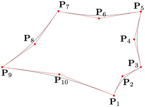
The vertex and half-edge records are illustrated in Figure 2a. The face records $f\in \mathcal{F}$ are best explained using an example, consider the DCEL in Figure 2b.

Figure 2. Illustrations of the vertex and half-edge records (left) and the face records (right).

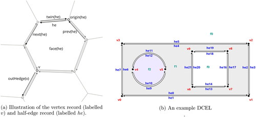
Each bounded face in the DCEL has one outer ring of half-edges that bound the face from the outside, for example face f₂ is bounded by $\{h{e}_{10},h{e}_{12}\}.$ Additionally, each bounded face may have an arbitrary number of rings that bound the face from the inside, in the case of f₁ these two rings are $\{h{e}_9,h{e}_{11}\}$ and $\{h{e}_{13},h{e}_{21},h{e}_{19},h{e}_{17}\}.$ A ring bounding a face will always be oriented such that the face will be to its left (w.r.t to the tangent vector). Therefore, outer rings run counter clockwise and inner rings will run clockwise. The unbounded face, which in this paper will always be defined as f₀, is a face used to delineate the boundary of the DCEL. This face stretches into infinity in all directions and is also the face bounded by any rings that form holes in the DCEL. In this paper all of the geometries will be assumed to be connected, therefore the unbounded face has exactly one inner ring that bounds it from the inside, in this case it is $\{h{e}_1,h{e}_7,h{e}_5,h{e}_3\}.$ The number of outer rings belonging to f₀ is equal to the number of holes in the DCEL, in this case there is just one hole and it is bounded by the ring $\{h{e}_{14},h{e}_{16},h{e}_{18},h{e}_{20}\}.$ To traverse the rings that bound it, each face need only store a reference to an arbitrary half-edge in each ring. The next() and prev() pointers may then by followed to traverse each ring. Each face record $f\in \mathcal{F}$ therefore stores the following (de Berg et al. 2008):

• An array of outer-ring half edges, for bounded faces this will have just one half-edge which is any half-edge in the outer ring that bounds f. For the unbounded face this array will have one half-edge for every hole in the domain and each. This array shall be denoted outerHedges(f).

• An array of inner-ring half edges, for bounded faces this may have any number of half-edges in it. For the unbounded face f₀ this will have just one half-edge. This array shall be denoted innerHedges(f).

For a given DCEL the face records are not unique, there would be many ways to describe the same DCEL. In the case of Figure 2b, a possible set of values for the face records could be that shown in Table 1 If the DCEL is in a valid state, with validity defined as being 2-manifold, then the DCEL will satisfy the Euler-Poincarè formula: (4.1) $$V-E+F=2(S-H)+R$$(4.1) where V, E, F, S, H and R are the number of vertices, edges, faces, shells, holes and rings respectively. In ${\mathbb{R}}^2$ a shell is simply a connected component of the DCEL. In this paper all geometries will consist of one connected component so S = 1. In the case of Figure 2b we have V = 10, E = 10, F = 3, H = 1 and R = 3. Using these values in Equation (4.1)(4.1) $$V-E+F=2(S-H)+R$$(4.1) gives $3=3,$ therefore the DCEL of Figure 2b is a valid 2-manifold geometry.

Table 1. Possible choice of half-edges for defining rings of face f₀.

Face	outerHedges(f)	innerHedges(f)
f0	he14	he5
f1	he0	$\{h{e}_{11},h{e}_{13}\}$
f2	he12	$\varnothing$

In this paper, Euler operators (Mantyla and Sulonen 1982; Mäntylä 1983; Mantyla 1984) are used to construct geometry. These operators add or remove vertices, edges, faces, shells, holes and rings in such a way as to preserve Euler-Poincarè formula at every stage (Mantyla and Sulonen 1982). The Euler operators serve as manipulation primitives which may be combined to form complex and intuitive geometric operations which are guaranteed to be 2-manifold. Although the terms of Equation (4.1)(4.1) $$V-E+F=2(S-H)+R$$(4.1) may only have positive integer values: if one were to briefly consider $(V,E,D,S,H,R)$ to be a vector in ${\mathbb{R}}^6,$ then the Euler-Poincarè formula may be thought of a hyperplane with normal vector $(1,-1,1,-2,2,-1).$ Under this interpretation, the Euler operators may be thought of as a set of 5 linearly independent vectors in ${\mathbb{R}}^6,$ with integer values, that span the hyperplane (Mäntylä 1983). There are many valid choices for this spanning set however the literature on Euler operators has converged to the set given in Table 2 (Mäntylä 1983).

Table 2. The set of 5 Euler operators and their inverses.

Operator	Meaning	V	E	F	S	H	R
mvsf	make vertex shell face	+1	0	+1	+1	0	0
kvsf	kill vertex shell face	−1	0	−1	−1	0	0
mev	make edge, vertex	+1	+1	0	0	0	0
kev	kill edge, vertex	−1	−1	0	0	0	0
mef	make edge, face	0	1	1	0	0	0
kef	make edge, face	0	−1	−1	0	0	0
mekr	make edge, kill ring	0	+1	0	0	0	−1
kemr	kill edge, make ring	0	−1	0	0	0	+1
Mfkrh	make face, kill ring, hole	0	0	+1	0	−1	−1
Kfmrh	kill face, make ring, hole	0	0	−1	0	+1	+1

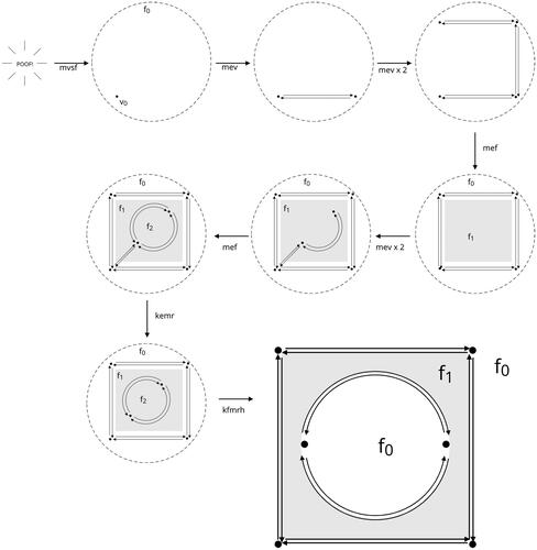
We demonstrate the use of Euler operators to build a square with a hole inside of it in Figure 3, this is one of the simplest geometries that uses all five operators.

Figure 3. The series of Euler operators used to create a DCEL representing a square with a hole in it.

Both the “mesh” and the “domain”, as they are commonly thought of in the FEM literature, are represented using the DCEL data-structure. The only difference between the mesh and the initial domain is that the mesh is subdivided into many more faces. To remain consistent with the FEM literature, the subscript h will be used to refer to the mesh. Therefore, the mesh shall be defined as a triple $({\mathcal{V}}_h,{\mathcal{E}}_h,{\mathcal{F}}_h)$ where ${\mathcal{V}}_h,{\mathcal{E}}_h$ and ${\mathcal{F}}_h$ have the same definitions as they did for the initial domain. All of the geometric information needed to implement the NE-VEM is stored in point field of each vertex $v\in {\mathcal{V}}_h$ and in thee curve field of each half-edge $he\in {\mathcal{E}}_h,$ this data is generated during mesh generation.

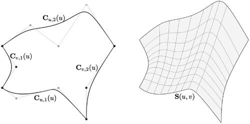
4.2. The NURBS polygon

The key to implementing the NURBS-enhanced VEM is to have a geometric description of curvilinear polygons which can serve as a base for numerical integration. To this end, the edges of the curvilinear polygon were encoded using NURBS curves and the polygon itself is tessellated into NURBS surfaces. NURBS are a standard description of geometry which are ubiquitous in computer-aided geometric design. The knot vector is a non-decreasing set of real numbers $\mathbf{u}=[u_1,\dots ,u_m]$ with each u_i referred to as a knot. Repeated knots are permitted and the number of times a knot appears in a knot vector is referred to as the knot multiplicity. The i’th half-open interval $[u_i,u_{i+1}),$ which may have zero length, are referred to as knot spans. From a given knot vector, a set of B-spline basis functions of polynomial order p (denoted $N_{i,p}(u)$) are using the Cox-deBoor recursion (Piegl and Tiller 1995; Cox 1972; de Boor 1972): $$\begin{array}{c}{N}_{i,0}(u)=\{\begin{array}{c}1\hspace{1em}\text{if}\hspace{1em}{u}_i\le u<u_{i+1}\hfill \\ 0\hspace{1em}\text{otherwise}\hfill \end{array},\hspace{1em}p=0\\ N_{i,p}(u)=\frac{u-u_i}{u_{i+p}-u_i}{N}_{i,p-1}(u)+\frac{u_{i+p+1}-u}{u_{i+p+1}-u_{i+1}}{N}_{i+1,p-1}(u),\hspace{1em}p>0\end{array}$$

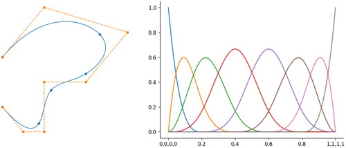
For a knot vector with m knots there will be $r=m-(p+1)$ basis functions of order p. Given r points in ${\mathbb{R}}^d,$ denoted ${\left\{{\mathbf{P}}_i\right\}}_{i=1}^r$ where d = 2, 3 and r corresponding wights ${\left\{w_i\right\}}_{i=1}^r,$ a p-order NURBS curve is defined as (Piegl and Tiller 1995): $$\mathbf{C}(u)=\sum _{i=1}^r{R}_i^p(u){\mathbf{P}}_i,\hspace{1em}\text{where}\hspace{1em}{R}_i^p(u)=\frac{w_i{N}_{i,p}(u)}{\sum _{j=1}^r{w}_j{N}_{j,p}(u)}.$$

NURBS curves are non-interpolatory, meaning that the curve does not pass through its control points unless the corresponding knot has a multiplicity of p. We give an example NURBS curve and the associated B-spline basis in Figure 4. If all the weights are equal then $R_i^p(u)=N_{i,p}(u)$ and the NURBS curve becomes the B-spline curve. Given two knot vectors $\mathbf{u}=[u_1,\dots ,u_m]$ and $\mathbf{v}=[v_1,\dots ,v_n],$ two polynomial orders p and q, a r-by-s 2D array of points ${\mathbf{P}}_{i,j}$ (where $r=m-(p+1)$ and $s=n-(q+1)$) and r-by-s 2D array of weights $w_{i,j}$ the NURBS surface is defined as (Piegl and Tiller 1995): $$\mathbf{S}(u,v)=\sum _{i=1}^r\sum _{j=1}^s{R}_{i,j}^{p,q}(u,v){\mathbf{P}}_{i,j},\hspace{1em}\text{where}\hspace{1em}{R}_{i,j}^{p,q}(u,v)=\frac{w_{i,j}{N}_{i,p}(u)N_{j,q}(v)}{\sum _{k=1}^r\sum _{l=1}^q{w}_{k,l}{N}_{k,p}(u)N_{l,q}(v)}$$ where ${\{N_{i,p}(u)\}}_{i=1}^r$ are the basis functions corresponding to u and ${\{N_{j,q}(v)\}}_{j=1}^s$ are the basis functions corresponding to v. Again, when all of the weights $w_{i,j}$ are equal then $R_{i,j}^{p,q}(u,v)=N_{i,p}(u)N_{j,q}(v)$ and the NURBS surface becomes a B-spline surface.

Figure 4. An example NURBS curve and its underlying B-spline basis.

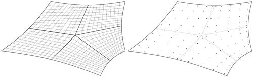
Given a curvilinear polygonal mesh there are two situations which arise when extracting polygons on which to perform local computations (such as computing local bilinear forms). The first case is where the polygon is not incident on any curved external boundaries or internal-interfaces (left polygon in Figure 5) and the second situation is where one or more of the polygon edges are incident on a curved external boundary or internal interface. In both cases, the objective is to have an NURBS description of the boundary of the polygon as a loop of NURBS curves and to also have a NURBS description of the interior of the polygon as a collection of NURBS surfaces.

Figure 5. A curvilinear mesh and an internal, all-straight polygon (left) and a boundary, curvilinear polygon (right).

Straight-sided polygon: In the straight-sided case each edge e_i between vertices ${\mathbf{v}}_i$ and ${\mathbf{v}}_{i+1}$ is represented with a linear B-spline curve: (4.2) $$p=1,\hspace{1em}\mathbf{u}=[0,0,1,1],\hspace{1em}\left\{{\mathbf{P}}_i\right\}=\left\{{\mathbf{v}}_i,{\mathbf{v}}_{i+1}\right\},\hspace{1em}\left\{w_i\right\}=\left\{1,1\right\}.$$(4.2) and the interior of each straight-sided polygon is modeled as a collection of bilinear NURBS surfaces (see Figure 6a) where the vertices of each surface S_i are the polygon vertex ${\mathbf{v}}_i,$ the midpoint of edge e_i which is denoted ${\mathbf{v}}_{e_i},$ the midpoint of edge $e_{i-1}$ denoted ${\mathbf{v}}_{e_{i-1}}$ and the centroid of the polygon denoted ${\mathit{x}}_F.$ Each S_i therefore has the following definition: (4.3) $$p=q=1,\hspace{1em}\mathbf{u}=\mathbf{v}=[0,0,1,1],\hspace{1em}\left\{{\mathbf{P}}_{i,j}\right\}=\left\{{\mathbf{v}}_i,{\mathbf{v}}_{e_i},{\mathbf{v}}_{e_{i-1}},{\mathit{x}}_f\right\},\hspace{1em}\left\{w_{i,j}\right\}=\left\{1,1,1,1\right\}.$$(4.3)

Figure 6. NURBS tesellations of the polygons highlighted in Figure 5.

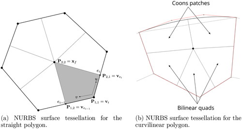
Curvilinear polygon: In the curvilinear case each edge e_i of the polygon is either a straight line defined using Equation (4.2)(4.2) $$p=1,\hspace{1em}\mathbf{u}=[0,0,1,1],\hspace{1em}\left\{{\mathbf{P}}_i\right\}=\left\{{\mathbf{v}}_i,{\mathbf{v}}_{i+1}\right\},\hspace{1em}\left\{w_i\right\}=\left\{1,1\right\}.$$(4.2) or is the curve segment of a boundary/internal-interface curve corresponding to a parameter interval $[u_l,u_h]\subset [0,1].$ During mesh generation, knot insertion is used to extract the curve segment corresponding to e_i from the boundary/internal-interface curve and the knot vector of the new curve e_i is reparameterised to span $[0,1]$ (see (Piegl and Tiller 1995) sections 5.2 and 6.4). The resulting curve segment is then stored in the curve field of the half-edge. After retrieving the curve fields for all $e_i\in \partial F$ from the DCEL, then the set of NURBS curves which bound the polygon have been defined. The surfaces S_i describing the interior of the curved polygon are either bilinear quads using Equation (4.3)(4.3) $$p=q=1,\hspace{1em}\mathbf{u}=\mathbf{v}=[0,0,1,1],\hspace{1em}\left\{{\mathbf{P}}_{i,j}\right\}=\left\{{\mathbf{v}}_i,{\mathbf{v}}_{e_i},{\mathbf{v}}_{e_{i-1}},{\mathit{x}}_f\right\},\hspace{1em}\left\{w_{i,j}\right\}=\left\{1,1,1,1\right\}.$$(4.3) if all their edges are straight lines or they are Coons surfaces if one or more of the boundary edges is curved (see Figure 6b). Coons surfaces, named after Steven A Coons (Coons 1967; Coons 1974), are interpolation surfaces which exactly conform to a set of four bounding curves. The Coons surface is defined as follows: (4.4) $$\mathbf{S}(u,v)=\sum _{i=1}^r\sum _{j=1}^s{R}_{i,j}^{p,q}(u,v){\mathbf{Q}}_{i,j}={\mathbf{S}}_1(u,v)+{\mathbf{S}}_2(u,v)+{\mathbf{S}}_3(u,v)$$(4.4) where ${\mathbf{S}}_1(u,v)$ is the ruled surface between ${\mathbf{C}}_{u,1}$ and ${\mathbf{C}}_{u,2},{\mathbf{S}}_2(u,v)$ is the ruled surface between ${\mathbf{C}}_{v,1}$ and ${\mathbf{C}}_{v,2}$ and ${\mathbf{S}}_3(u,v)$ is the bilinear quad with corners equal to the endpoints of the boundary curves. $${\mathbf{S}}_1(u,v)={\mathbf{C}}_{1,u}(u)+(1-v){\mathbf{C}}_{2,u}(u),\hspace{1em}{\mathbf{S}}_2(u,v)={\mathbf{C}}_{1,v}(v)+(1-u){\mathbf{C}}_{2,v}(v).$$

The steps necessary to construct a Coons surface are to find the orders p and q, knot vectors u and v, control points ${\mathbf{Q}}_{i,j}$ and weights $w_{i,j}$ such that Equation (4.4)(4.4) $$\mathbf{S}(u,v)=\sum _{i=1}^r\sum _{j=1}^s{R}_{i,j}^{p,q}(u,v){\mathbf{Q}}_{i,j}={\mathbf{S}}_1(u,v)+{\mathbf{S}}_2(u,v)+{\mathbf{S}}_3(u,v)$$(4.4) is satisfied (Figure 7).

Figure 7. A loop of four bounding curves (left) and the resulting Coons surface.

The order p in the u-parameter is the maximum of the orders of ${\mathbf{c}}_{1,u}$ and ${\mathbf{c}}_{2,u}$ and the knot vector u is the merger knot vectors of ${\mathbf{c}}_{1,u}$ and ${\mathbf{c}}_{2,u}$ (denoted ${\mathbf{u}}_1,{\mathbf{u}}_2$). This means that if knot $u_i\in {\mathbf{u}}_1$ or $u_i\in {\mathbf{u}}_2$ then $u_i\in \mathbf{u}$ and the maximum multiplicity of u_i in either ${\mathbf{u}}_1$ or ${\mathbf{u}}_2$ is inherited by u (Piegl and Tiller 1995, Section 8.4). The same steps are performed with ${\mathbf{c}}_{1,v}$ and ${\mathbf{c}}_{2,v}$ to find order q and knot vector v. Next, through a mixture of order-elevation and knot-insertion (see Piegl and Tiller 1995, Chapter 5) the knot vectors of ${\mathbf{S}}_1,{\mathbf{S}}_2$ and ${\mathbf{S}}_3$ are made to be equal to u and v. After this step, the number of control points/weights in each surface are equal. We may then follow the method presented in (Lin and Hewitt 1994) for finding the control points and weights in homogenous coordinates. For the internal points in the control net (so for all $(i,j)\in \left\{2,\dots ,r-1\right\}\times \left\{2,\dots ,s-1\right\})$ we have: $$\left[\begin{array}{c}{w}_{i,j}{\mathbf{Q}}_{i,j}\\ w_{i,j}\end{array}\right]=\left[\begin{array}{c}{w}_{i,j}^1{\mathbf{P}}_{i,j}^1+w_{i,j}^2{\mathbf{P}}_{i,j}^2-w_{i,j}^3{\mathbf{P}}_{i,j}^2\\ w_{i,j}^1+w_{i,j}^2-w_{i,j}^3\end{array}\right].$$ and for all boundary control points (so for all (i, j) where $i=1,r$ or $j=1,s$) $$\left[\begin{array}{c}{w}_{i,j}{\mathbf{Q}}_{i,j}\\ w_{i,j}\end{array}\right]=\left[\begin{array}{c}{w}_{i,j}^1{w}_{i,j}^2\left({\mathbf{P}}_{i,j}^1+{\mathbf{P}}_{i,j}^2-{\mathbf{P}}_{i,j}^3\right)\\ w_{i,j}^1{w}_{i,j}^2\end{array}\right].$$

5. Integration on curvilinear polygons

Accurate integration on curvilinear polygons is accomplished using one of two methods: Lasserre’s Method (Lasserre 1998) for homogenous functions and a Subtessellation Method for non-homogenous functions. Lassere’s Method makes use of the NURBS boundary curves computed in Section 4.2 while the subtessellation method, as the name suggests, makes use of the NURBS surface representation of the interior of the polygon also computed in Section 4.2. Using the exact-geometry information encoded by the NURBS curves and surfaces means that the geometric error is eliminated and the VEM attains the theoretical order of accuracy for problems with curved domains.

The motivation for presenting two methods of integration is that each method performs a separate function within the VEM implementation presented in this paper.

Lassere’s method is very computationally efficient for computing integrals of families of scaled monomials up to a given order. Therefore, it greatly accelerates the computation of matrices containing scaled monomial inner products ${(m_{\alpha },m_{\beta })}_{0,F}$ and $(\nabla m_{\alpha },\nabla m_{\beta }).$ These inner products are necessary to construct the local VEM bilinear forms, for more details as to why this is the case the author should consult (Beirão da Veiga et al. 2014)).

The subtessellation method of integration is required to integrate non-homogeneous functions on curvilinear polygons, the most important application of which the computation of source terms of the form: ${(f(\mathit{x}),{\phi }_i)}_{0,F}$ where $f(\mathit{x})$ is a prescribed extraneous source.

5.1. Lasserre’s method

Lassere’s method was first presented in (Lasserre 1998) and is a method of converting integrals of homogeneous functions over a volume (polyhedra in 3D and polygons in 2D) into the sum of integrals over surfaces (polygons in 3D and edges in 2D). In (Chin, Lasserre, and Sukumar 2015) the authors extended Lassere’s original method to include non-convex polygons and polyhedra. Finally, in (Antonietti, Manzini, et al. 2018) the authors applied the method presented in (Chin, Lasserre, and Sukumar 2015) to develop very efficient recursive algorithm to compute all of the monomials up to a given order on arbitrary polygons/polyhedra. In this paper we implemented the algorithm presented in (Antonietti, Manzini, et al. 2018) however we modified it to also handle curvilinear polygons. This section shall review the theory and the pseudocode of our algorithm is given in the Appendix A.1.

Definition 5.1.

Homogeneous function. A homogenous function $g(\mathit{x}):{\mathbb{R}}^d\to {\mathbb{R}}^{}$ of degree q is any function that satisfies: $$g(\lambda \mathit{x})={\lambda }^{q}g(\mathit{x}),$$

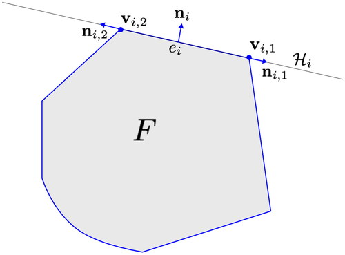
Monomials fall into this class of function therefore many computations in VEM are greatly accelerated by Lasserre’s Method. Consider a polygon $F\subset {\mathbb{R}}^2$ which has a boundary $\partial F$ made up of a set of curvilinear edges ${\widehat{\mathcal{E}}}_F$ and straight edges ${\mathcal{E}}_F.$ Using the terminology and notation of (Antonietti, Manzini, et al. 2018) each straight edge is a subset of a hyperplane in ${\mathbb{R}}^2$ defined as: $$e_i\subset {\mathcal{H}}_i=\left\{\mathit{x}\in {\mathbb{R}}^2:\mathit{x}.{\mathbf{n}}_i=b_i\right\}$$ where ${\mathbf{n}}_i$ is the outward unit-normal vector of edge e_i the and b_i is the perpendicular distance of the hyperplane from the origin, see Figure 8 for an example.

Figure 8. Polygon F with an example hyperplane ${\mathcal{H}}_i.$ This is a recreation of ((Antonietti, Manzini, et al. 2018) Figure 1).

Lasserre’s Method makes use of two results from vector calculus: the first is Euler’s homogeneous function theorem, which states that for a homogeneous function of degree q the following identity holds: (5.1) $$qg(\mathit{x})=\nabla g(\mathit{x})·\mathit{x},$$(5.1) the second result is generalized Stokes’ Theorem which states for a vector field $\mathbf{f}:F\to {\mathbb{R}}^d$ that: (5.2) $${\int }_F\nabla ·\mathbf{f}g(\mathit{x})dx+{\int }_F\mathbf{f}·\nabla g(\mathit{x})dx={\int }_{\partial F}\mathbf{f}·\mathbf{n}g(\mathit{x})ds.$$(5.2)

Choosing the vector field to be $\mathbf{f}=\mathit{x}$ and substituting Equation (5.1)(5.1) $$qg(\mathit{x})=\nabla g(\mathit{x})·\mathit{x},$$(5.1) into Equation (5.2)(5.2) $${\int }_F\nabla ·\mathbf{f}g(\mathit{x})dx+{\int }_F\mathbf{f}·\nabla g(\mathit{x})dx={\int }_{\partial F}\mathbf{f}·\mathbf{n}g(\mathit{x})ds.$$(5.2) yields Lasserre’s method for homogenous functions: (5.3) $${\int }_{F}g(\mathit{x})dx=\frac{1}{2+q}{\int }_{\partial F}\mathit{x}·\mathbf{n}g(\mathit{x})ds=\frac{1}{2+q}\left[\sum _{e_i\in {\widehat{\mathcal{E}}}_F}{\int }_{e_i}\mathit{x}·\mathbf{n}g(\mathit{x})ds+\sum _{e_i\in {\mathcal{E}}_F}{b}_i{\int }_{e_i}g(\mathit{x})ds\right]$$(5.3)

For all curvilinear edges $e_i\in {\widehat{\mathcal{E}}}_F$ direct integration is performed using Gauss-Legendre quadrature on the underlying NURBS curve, which assumed to be defined on $[0,1].$ Denoting the NURBS curve parameterization as $\mathbf{c}(t),$ the quadrature is computed as follows: $${\int }_{e_i}\mathit{x}·\mathbf{n}g(\mathit{x})ds={\int }_0^1\mathbf{c}(t)·\mathbf{n}(t)g\left(\mathbf{c}(t)\right)|J(t)|dt\approx \sum _{i=1}^{\text{nqp}}\mathbf{c}(t_i)·\mathbf{n}(t_i)g(\mathbf{c}(t_i))w_i|J(t_i)|$$ where t_i, w_i are the quadrature points and weights respectively and $\mathbf{n}(t)$ and J(t) are: $$\mathbf{n}(t)=\frac{d\mathbf{c}(t)}{dt}{\Vert \frac{d\mathbf{c}(t)}{dt}\Vert }_{{\mathbb{R}}^2}^{-1},\hspace{1em}J(t)=\sqrt{\frac{d\mathbf{c}(t)}{dt}·\frac{d\mathbf{c}(t)}{dt}}$$

The full quadrature rule on a curve is computed by mapping a standard Gauss-Lobatto quadrature defined in $[-1,1]$ to each non-zero length knot span $[u_i,u_{i+1})\subset [0,1].$ So, given a knot vector with M non-zero knot spans and a quadrature rule with m points then $\text{nqp}=m\times M.$ This is a simplistic way to generate quadrature points for NURBS curves and more efficient methods exist (Hughes, Reali, and Sangalli 2010) which take into account continuity of the B-spline basis. However, the vast majority of edges in the EG-mesh are straight lines so the additional computational cost of this quadrature is negligible.

For all straight edges $e_i\in {\mathcal{E}}_F$ we follow the technique introduced in (Lasserre 1998; Chin, Lasserre, and Sukumar 2015), whereby Lasserre’s Method is applied recursively to each straight edge in Equation (5.3)(5.3) $${\int }_{F}g(\mathit{x})dx=\frac{1}{2+q}{\int }_{\partial F}\mathit{x}·\mathbf{n}g(\mathit{x})ds=\frac{1}{2+q}\left[\sum _{e_i\in {\widehat{\mathcal{E}}}_F}{\int }_{e_i}\mathit{x}·\mathbf{n}g(\mathit{x})ds+\sum _{e_i\in {\mathcal{E}}_F}{b}_i{\int }_{e_i}g(\mathit{x})ds\right]$$(5.3) . Using the notation of Figure 8, if we define ${\mathit{x}}_{0,i}={\mathbf{v}}_{i,1}$ to be the origin of ${\mathcal{H}}_i$ we have: $${\int }_{e_i}g(\mathit{x})dx=\frac{1}{(1+q)}\left[\left|e_i\right|g({\mathbf{v}}_{i,2})+{\int }_{e_i}{\mathbf{v}}_{i,1}·\nabla g(\mathit{x})ds\right].$$

If $g(\mathit{x})$ is polynomial then the term ${\mathbf{v}}_{i,1}.\nabla g(\mathit{x})$ is a polynomial of lower order. This property of polynomials lends itself to the design of a recursive algorithm for computing the integrals of families of monomials up to a specified order. In (Antonietti, Manzini, et al. 2018) one such recursive algorithm was presented and has been slightly modified here to allow for polygons with curvilinear edges. The problem which was solved in (Antonietti, Manzini, et al. 2018) is is to compute the array: $$I_p^F=\left[{\int }_F{m}_{1}dx,{\int }_F{m}_{2}dx,\dots ,{\int }_F{m}_{n_p}dx\right],\hspace{1em}{m}_{\alpha }(\mathit{x})\in {\mathcal{M}}_p(F)$$ as efficiently as possible and without simply resorting to direct quadrature. Before detailing the algorithm a quick review of properties of scaled monomials is needed.

Property 5.2.

Let $\widehat{F}$ be the same as F but translated by $-{\mathit{x}}_F.$ Therefore, ${\mathit{x}}_{\widehat{F}}=\mathbf{0}.$ The following identity holds: $${\int }_F{m}_i(\mathit{x})dx=\frac{1}{h_{\widehat{F}}^{{\alpha }_x+{\alpha }_y}}{\int }_{\widehat{F}}{u}_i(\mathit{x})dx\hspace{1em}\mathit{\text{where}}\hspace{1em}{u}_i(\mathit{x})=x^{{\alpha }_x}{y}^{{\alpha }_y}$$

Property 5.3.

The derivative of a monomial of order p is another monomial of order p – 1, recalling the single index to multi-index mapping of Equation (2.1)(2.1) $$1\iff (0,0),\hspace{1em}2\iff (1,0),\hspace{1em}3\iff (0,1),\hspace{1em}4\iff (2,0),\hspace{1em}5\iff (1,1),\hspace{1em}6\iff (0,2),\dots$$(2.1) , $\alpha (i,j):{\mathbb{N}}^2\to \mathbb{N}$ we have: $$\frac{\partial }{\partial x}{u}_{\alpha (a,b)}(\mathit{x})=a{u}_{\alpha (a-1,b)}(\mathit{x})\hspace{1em}\mathit{\text{and}}\hspace{1em}\frac{\partial }{\partial y}{u}_{\alpha (a,b)}(\mathit{x})=b{u}_{\alpha (a,b-1)}(\mathit{x})$$

Property 5.2 is crucial if one wishes to used Lassere’s Method as $u_i(\mathit{x})$ is homogenous and $m_i(\mathit{x})$ is not. Algorithms 1 to 4 in the appendix present the full algorithm for computing $I_p^F$ using the method presented in this section.

Once the array of scaled monomial integrals has been computed it may be stored and used to compute many important quantities in VEM, most notably the inner products ${(m_i,m_j)}_{0,F}$ and ${(\nabla m_i,\nabla m_j)}_{0,F}.$ For example, let’s say $m_i(\mathit{x})$ has exponents (a, b) and $m_j(\mathit{x})$ has exponents (c, d) then $m_i(\mathit{x})m_j(\mathit{x})=m_l(\mathit{x})$ where $l=\alpha (a+c,b+d).$ Therefore, the inner product of these two monomials will already have been computed and stored in $I_p^F[l].$ A similar approach may be employed to compute ${(\nabla m_i,\nabla m_j)}_{0,F}$ by making use of property 5.3.

5.2. Subtessellation method

If the integrand $f(\mathit{x})$ is not homogeneous i.e. does not satisfy Equation 5.1(5.1) $$qg(\mathit{x})=\nabla g(\mathit{x})·\mathit{x},$$(5.1) , then the method of integration used in this paper is the Subtessellation Method. Let us assume that polygon F has been decomposed into a set of (possibly curvilinear) NURBS quads S_i using one of the methods given in the previous section: $$F=\underset{i=1}{\overset{N_e^F}{\cup }}{S}_i\hspace{1em}\text{where}\hspace{1em}{S}_i=\left\{\mathit{x}\in {\mathbb{R}}^2:\mathit{x}={\mathbf{S}}_i(u,v)\hspace{1em}\forall (u,v)\in {[0,1]}^2\right\}.$$

Then tensor-product Gauss-Legendre quadrature rules of any required order may be generated on ${[0,1]}^2$ and then mapped onto each NURBS surface S_i. An example is presented in Figure 9.

Figure 9. An example curvilinear polygon (left), its NURBS tessellation (middle) and its quadrature points (right).

The integral of $f(\mathit{x})$ may be computed as follows: $${\int }_{F}f(\mathit{x})dx=\sum _{i=1}^{N_e^F}{\int }_{S_i}f(\mathit{x})dx=\sum _{i=1}^{N_e^F}{\iint }_{{[0,1]}^2}f({\mathbf{S}}_i(u,v))J_i(u,v) du dv$$ where $J_i(u,v)$ is the surface Jacobian given by: $$J_i(u,v)=\text{det}\left({\mathbf{J}}_i(u,v)\right),\hspace{1em}\text{where}\hspace{1em}{\mathbf{J}}_i(u,v)=\left[\frac{\partial {\mathbf{S}}_i(u,v)}{\partial u}\frac{\partial {\mathbf{S}}_i(u,v)}{\partial v}\right].$$

Let ${\left\{u_l\right\}}_{l=1}^{{\text{nqp}}_u}$ denote the ${\text{nqp}}_u$ Gauss-Legendre points on $[0,1]$ for the u surface parameter, let ${\left\{v_m\right\}}_{m=1}^{{\text{nqp}}_v}$ denote the ${\text{nqp}}_v$ Gauss-Legendre points on $[0,1]$ for the v surface parameter and let $w_{l,m}=w_l{w}_m$ denote the weight at point $(u_l,v_m)$ then the integral over each NURBS surface of the subtessellation may be written as: $${\iint }_{{[0,1]}^2}f({\mathbf{S}}_i(u,v))J_i(u,v) du dv\approx \sum _{l=1}^{{\text{nqp}}_u}\sum _{m=1}^{{\text{nqp}}_v}f\left({\mathbf{S}}_i(u_l,v_m)w_{l,m}J(u_l,v_m)\right)$$

The subtessellation method presented here is an alternative to method of integration presented in (Beirão da Veiga, Russo, and Vacca 2019; Sommariva and Vianello 2007), which does not require subtessellation but rather uses Green’s integration formula to convert an integral of function $f(\mathit{x})$ over the polygon into an integral of the antiderivative $F(\mathit{x})$ over the boundary. The values of the the antiderivative at the boundary quadrature points are then generated by integrating $f(\mathit{x})$ along a line perpendicular to a” base line” and incident on the boundary quadrature point (Sommariva and Vianello 2007).

6. Numerical results

In this this section shall present a series of numerical tests to demonstrate the key features of the NECG-VEM. Specifically, the optimal rates of convergence under h-refinement for curvilinear polygonal meshes and improved rates of convergence in integral quantities (such as scalar neutron flux integrals) for nuclear reactor physics problems with curvilinear domains.

As a practical matter, when comparing the NECG-VEM to the classical CG-VEM, we represent linear polygonal meshes with the same DCEL-plus-NURBS representation described in Section 4. The only difference is that we restrict the NURBS curves attached to half-edges to be linear NURBS representing a straight lines between two points. Additionally, as we mentioned in Section 2, the classical CG-VEM local space and the local NECG-VEM space coincide when the polygon is linear. Therefore, we do not have a separate implementation of the classical VEM, it is simply a special case of the NECG-VEM when all edges in the mesh are assigned linear NURBS curves. Consequently, the classical CG-VEM on linear polygonal meshes is just a special case of the NECG-VEM, thus avoiding the need to maintain two separate VEM codes.

In Section A.3 we provide detail on how the linear meshes approximate curves, with one implementation simply interpolating curves with line segments, which we call the non-area-preserved linear mesh as in this case the areas of material subdomains will be incorrect relative to the geometry. In the second implementation we displace the vertices of the mesh in such a way as to force the area to be preserved. We shall refer to this second case as the area-preserved linear mesh.

All polygonal meshes, both curvilinear and linear, used in this paper were generated using our own mesh-generator which we developed as part of this research. The mesh generator itself uses the centroidal Voronoi tessellation to decompose the domain. However, a full description of the mesh generator is outside the scope of this paper.

6.1. Quadrature comparison

The comparison between Lassere’s Method and subtessellation quadrature, both in terms of integral errors and computational complexity, was thoroughly investigated in (Antonietti, Manzini, et al. 2018) for straight-sided polygons and polyhedra when computing families of monomials up to a prescribed order. In this section, we shall provide a brief comparison of the subtessellation method and Lessere’s method for computing all of the scaled monomials up to order p = 4 on a curvilinear polygon where all edges are NURBS curves. The purpose of this section is to demonstrate that both methods yield the same results to within very narrow margin of one another: a relative difference of less than $1\times {10}^{-8}$ in most cases. The curvilinear polygon used for this test is presented in Figure 10.

Figure 10. Curvilinear polygon used in this test case, left image shows the NURBS surface tessellation and the right image shows a substessellation quadrature set of order p = 8.

Let $I_L(m_i)$ and $I_S(m_i)$ denote the Lassere and subtessellation approximations to the integral: ${\int }_F{m}_i(\mathit{x})dx$ respectively and let the relative difference between them be: $$\delta (m_i)=\frac{|I_L(m_i)-I_S(m_i)|}{|I_L(m_i)|}$$

The values of $I_L(m_i),I_S(m_i)$ and $\delta (m_i)$ are tabulated in Table 3 up to order p = 4. In the supplementary data we also show that $\delta (m_i)$ stays low (around $1\times {10}^{-8}$) up to order p = 10. The conclusion we may draw from Table 3 is that the use of Lassere’s method to compute scaled monomial integrals on NURBS polygons does not incur a significant integration error when compared to direct subtessellation quadrature. The curvilinear polygon presented in this section also represents a worst-case scenario in that all of the edges are curvilinear. In practice no more than two edges in a given polygon are curvilinear (Figure 11).

Figure 11. The domain, $V=V_1\cup V_2$ used for this MMS test case.

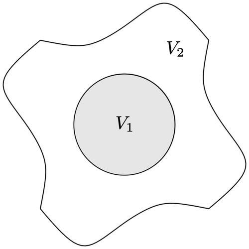
Table 3. Comparison of integrals of scaled monomials up to p = 4.

Scaled monomial	$({\alpha }_1,{\alpha }_2)$	$I_L(m_i)$	$I_S(m_i)$	$\delta (m_i)$
m1	(0, 0)	9.2185e + 00	9.2185e + 00	6.4745e-13
m2	(1, 0)	−6.7486e-06	−6.7486e-06	3.5886e-07
m3	(0, 1)	3.7531e-06	3.7531e-06	2.0452e-07
m4	(2, 0)	4.1114e-01	4.1114e-01	3.9477e-11
m5	(1, 1)	2.2870e-02	2.2870e-02	5.5856e-11
m6	(0, 2)	1.5331e-01	1.5331e-01	3.5220e-11
m7	(3, 0)	−2.2822e-02	−2.2822e-02	5.0147e-10
m8	(2, 1)	−3.3880e-03	−3.3880e-03	1.7617e-10
m9	(1, 2)	6.8550e-03	6.8550e-03	1.4924e-10
m10	(0, 3)	8.8397e-04	8.8397e-04	1.4388e-09
m11	(4, 0)	3.9709e-02	3.9709e-02	8.7052e-10
m12	(3, 1)	4.9559e-03	4.9559e-03	4.0976e-12
m13	(2, 2)	5.4515e-03	5.4515e-03	6.6281e-10
m14	(1, 3)	1.2520e-04	1.2520e-04	6.7278e-09
m15	(0, 4)	5.1892e-03	5.1892e-03	7.3321e-10

6.2. Method of manufactured solutions

Consider the following geometry comprised of two subdomains V₁ and V₂ shown below:

The following two-group problem is defined on $V=V_1\cup V_2.$ (6.1) $$\{\begin{array}{cc}-\nabla .\left(D^1\nabla {\varphi }_1\right)+{\Sigma }_r^1{\varphi }_1=f_1\hfill & \hspace{1em}\forall \mathit{x}\in V\hfill \\ -\nabla .\left(D^2\nabla {\varphi }_2\right)+{\Sigma }_r^2{\varphi }_2=f_2+{\Sigma }_s^{1\to 2}{\varphi }_1\hfill & \hspace{1em}\forall \mathit{x}\in V\hfill \\ -D^1\nabla {\varphi }_1.\mathbf{n}=r_1\hfill & \hspace{1em}\forall \mathit{x}\in \partial V\hfill \\ -D^2\nabla {\varphi }_2.\mathbf{n}=r_2\hfill & \hspace{1em}\forall \mathit{x}\in \partial V\hfill \end{array}.$$(6.1)

The values of the material coefficients may be found in the appendix, Table 7. Letting $v=(v_1,v_2)\in {\left[H^1(V)\right]}^2,$ $\varphi =({\varphi }_1,{\varphi }_2)\in {\left[H^1(V)\right]}^2$ and $f=(f_1,f_2),$ Equation (6.2)(6.2) $$\{\begin{array}{c}\text{Find}\mathrm{ }\varphi \in {\left[H^1\left(V\right)\right]}^2\text{such}\mathrm{ }\text{that}\\ A(v,\varphi )=l\left(v\right)\hspace{1em}\forall v\in {\left[H^1\left(V\right)\right]}^2\end{array},$$(6.2) has the following variational form: (6.2) $$\{\begin{array}{c}\text{Find}\mathrm{ }\varphi \in {\left[H^1\left(V\right)\right]}^2\text{such}\mathrm{ }\text{that}\\ A(v,\varphi )=l\left(v\right)\hspace{1em}\forall v\in {\left[H^1\left(V\right)\right]}^2\end{array},$$(6.2) where $$A(v,\varphi )=\hspace{1em}\begin{array}{c}{(\nabla v_1,D^1\nabla {\varphi }_1)}_{0,V}+{(v_1,{\Sigma }_r^1{\varphi }_1)}_{0,V}\\ +\\ {(\nabla v_2,D^2\nabla {\varphi }_2)}_{0,V}+{(v_2,{\Sigma }_r^2{\varphi }_2)}_{0,V}-{(v_2,{\Sigma }_s^{1\to 2}{\varphi }_1)}_{0,V}\end{array}$$ and $$l(v)={(v_1,f_1)}_{L^2(V)}+{(v_1,r_1)}_{\partial V}+{(v_2,f_2)}_{L^2(V)}+{(v_2,r_2)}_{\partial V}.$$

Table 7. Table of macroscopic nuclear cross section material data.

	D^1	D^2	${\Sigma }_r^1$	${\Sigma }_r^2$	${\Sigma }_s^{1\to 2}$
V1	2.0	3.0	0.5	0.9	0.2
V2	4.0	6.0	1.2	1.4	0.4

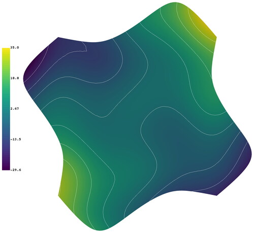
The source functions (f₁, f₂), derived in Section A.4, and boundary functions (r₁, r₂) are selected such that the exact solutions are given by the same function below: (6.3) $${\widehat{\varphi }}_1={\widehat{\varphi }}_2=\left(x+\hspace{0.17em}\text{cos}\hspace{0.17em}(y)\right)\left(y-\hspace{0.17em}\text{sin}\hspace{0.17em}(x)\right).$$(6.3)

Equation (6.3)(6.3) $${\widehat{\varphi }}_1={\widehat{\varphi }}_2=\left(x+\hspace{0.17em}\text{cos}\hspace{0.17em}(y)\right)\left(y-\hspace{0.17em}\text{sin}\hspace{0.17em}(x)\right).$$(6.3) is plotted in Figure 12.

Figure 12. Plot of the MMS solution, Equation (6.6), with isolines in white.

The variational form in Equation (6.2)(6.2) $$\{\begin{array}{c}\text{Find}\mathrm{ }\varphi \in {\left[H^1\left(V\right)\right]}^2\text{such}\mathrm{ }\text{that}\\ A(v,\varphi )=l\left(v\right)\hspace{1em}\forall v\in {\left[H^1\left(V\right)\right]}^2\end{array},$$(6.2) was solved for VEM orders orders $p=1,2,3,4,5$ and for two sets of successively more refined polygonal meshes. The first were curvilinear meshes which were used in conjunction with the NECG-VEM and the second were linear meshes which were used in conjunction with the classical CG-VEM. In the linear meshes, curves were approximated with a series of line segments where the start and end points lie on the curve (see Section A.3 for more detail). Therefore, the surface areas of V₁ and V₂ will be under-approximated by the mesh. Some examples of curvilinear meshes are given in Figure 13. Let h be the average element diameter for a given mesh and let ${\varphi }_1^h$ and ${\varphi }_2^h$ be the discrete VEM solutions to Equation (6.2)(6.2) $$\{\begin{array}{c}\text{Find}\mathrm{ }\varphi \in {\left[H^1\left(V\right)\right]}^2\text{such}\mathrm{ }\text{that}\\ A(v,\varphi )=l\left(v\right)\hspace{1em}\forall v\in {\left[H^1\left(V\right)\right]}^2\end{array},$$(6.2) then for every diameter-order pair, denoted (h, p), both the $L^2(V)$ and $H^1(V)$ errors were computed as follows: $$E_{L^2}\left({\varphi }_1^h\right)={\left(\sum _{F\in {\mathcal{T}}_h^{}}{\int }_F\left({\widehat{\varphi }}_1-{\Pi }_p^0{\varphi }_1^h\right)\left({\widehat{\varphi }}_1-{\Pi }_p^0{\varphi }_1^h\right)dx\right)}^{\frac{1}{2}},$$ and $$E_{H^1}({\varphi }_1^h)={\left(\sum _{F\in {\mathcal{T}}_h^{}}{\int }_F\left(\nabla {\widehat{\varphi }}_1-{\Pi }_{p-1}^0\nabla {\varphi }_1^h\right).\left(\nabla {\widehat{\varphi }}_1-{\Pi }_{p-1}^0\nabla {\varphi }_1^h\right)dx\right)}^{\frac{1}{2}},$$ with the errors for ${\varphi }_2^h$ having the same definition. Given that the exact solutions ${\widehat{\varphi }}_1$ and ${\widehat{\varphi }}_2$ are infinitely differentiable everywhere in V then the both ${\varphi }_1^h$ and ${\varphi }_2^h$ should converge with $\mathcal{O}(h^p)$ and $\mathcal{O}(h^{p+1})$ accuracy in the H¹ and L² norms respectively. Figure 14a and b presents the $L^2(V)$ and $H^1(V)$ errors for the curvilinear meshes with the NECG-VEM As may be seen, the expected order of accuracy is attained. Figure 15a and b plots the errors with the set of non-area-preserved linear meshes solved using the classical CG-VEM. In this case the errors at higher orders (orders >2 for the L² error and orders >3 for the H¹) are dominated by the geometric error. The rates of convergence for these higher orders are therefore limited to the rate of convergence of the geometric error, which is apparently $\mathcal{O}(h^2)$ for the L² error and $\mathcal{O}(h^3)$ for the H¹ error.

Figure 13. Three of the polygonal meshes used to solve Equation (6.3)(6.3) $${\widehat{\varphi }}_1={\widehat{\varphi }}_2=\left(x+\hspace{0.17em}\text{cos}\hspace{0.17em}(y)\right)\left(y-\hspace{0.17em}\text{sin}\hspace{0.17em}(x)\right).$$(6.3) .

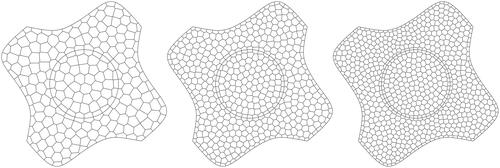
Figure 14. The errors $E_{L^2}$ and $E_{H^1}$ for the case where both exact geometry and polynomial basis orthogonalisation are enable.

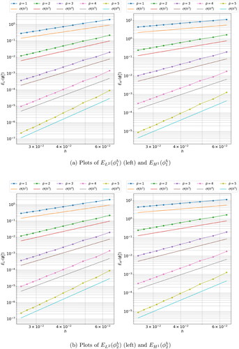
Figure 15. The errors $E_{L^2}$ and $E_{H^1}$ for the case where exact geometry has been disabled.

6.3. Burnable supercell benchmark verification test case

This problem, originally presented in (Wood and Williams 1984) and modified in (Owens, Kópházi, and Eaton 2017a), is a single group, extraneous, prescribed (or fixed) neutron source problem consisting of 8 identical fuel pins arranged around a central burnable absorber pin. A schematic of the geometry is presented in Figure 16 along with two of the curvilinear polygonal meshes used to solve this problem.

Figure 16. The geometry of the burnable supercell problem (left) and a curvilinear polygonal mesh with 3759 faces (middle) and 6863 faces (right).

Reflected boundary conditions are prescribed on all four sides of the supercell. The values of the neutron macroscopic neutron cross sections and the value of the extraneous, prescribed (fixed) neutron source $q(\mathit{x})$ are given in Table 4. Additionally, the scalar neutron flux contour of the reference solution is presented in Figure 17.

Figure 17. The scalar neutron flux contour of the reference solution.

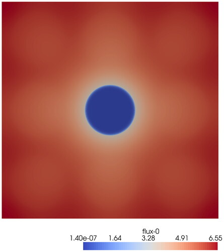
Table 4. The nuclear data for the burnable supercell benchmark verification test case.

Material	D	Σt	Σs	q
Moderator	0.4411	0.7557	0.7504	1
Fuel	0.6479	0.5145	0.3432	0
Absorber 1 (annulus)	1.5411e-02	21.630	0.3414	0
Absorber 2 (circle)	2.3359e-02	14.270	0.3400	0

The governing equations of this problem are: $$\{\begin{array}{cc}-\nabla .\left(D(\mathit{x})\nabla \varphi (\mathit{x})\right)+{\Sigma }_a(\mathit{x})\varphi (\mathit{x})=q(\mathit{x})\hfill & \hspace{1em}\forall \mathit{x}\in V\subset {\mathbb{R}}^2\hfill \\ -D(\mathit{x})\nabla \varphi (\mathit{x}).\mathbf{n}=0\hfill & \hspace{1em}\forall \mathit{x}\in \partial V\hfill \end{array}$$ where $D=1/3{\Sigma }_t$ and ${\Sigma }_a={\Sigma }_t-{\Sigma }_s.$ Qualitatively, the solution in Figure 17 behaves as one would expect. It is flat and smooth far away from the moderator-absorber interface while at the interface the solution exhibits a large gradient in the scalar neutron flux radially out from the center. The cause of this feature of the solution is the large change in the macroscopic absorption neutron cross section. Finally, the solution is symmetric with 45 degree symmetry. We shall define four quantities of interest (QoIs) for this problem:

• The integral of the scalar neutron flux over the moderator $I_{\text{mod}}.$

• The integral of scalar neutron flux over all eight fuel pins $I_{\text{fuel}}.$

• The integral of scalar neutron flux over the absorber annulus $I_{\text{ab}1}.$

• The integral of the scalar neutron flux over the absorber pin $I_{\text{ab}2}.$

The reference values for these quantities are shown in Table 5.

Table 5. The reference values of the QoIs.

QoI	$I_{\text{mod}}$	$I_{\text{fuel}}$	$I_{\text{ab}1}$	$I_{\text{ab}2}$
Reference value	1.24426023e + 02	7.21396107e + 01	4.09144631e-01	1.42273066e-03

They were computed using an NE-VEM scheme defined on a curvilinear polygonal mesh with 14038 elements and VEM order p = 4, resulting in a scheme with $N_{\text{gdof}}=231927.$

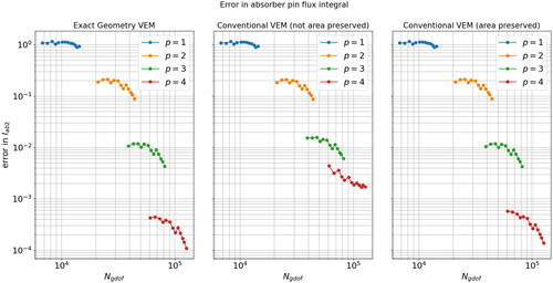
To generate the error curves shown in Figures 18–21 we solved the burnable supercell problem for VEM orders $p=1,2,3,4$ and for three separate sets of polygonal meshes. The first mesh set was curvilinear and exactly represented the geometry of the burnable supercell from the lowest level of mesh refinement. The second mesh series was linear and was not area-preserved, and the third and final mesh series was also linear but the mesh was area-preserved. The curvilinear mesh was used in conjunction with the NECG-VEM while the two linear meshes were used in conjunction with the classical CG-VEM.

Figure 18. Convergence plots of $I_{\text{mod}}$ for the exact-geometry VEM (left), the non-area-preserved classical VEM (middle) and area-preserved classical VEM (right).

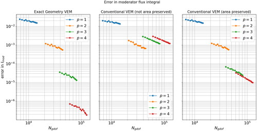
Figure 19. Convergence plots of $I_{\text{fuel}}$ for the exact-geometry VEM (left), the non-area-preserved classical VEM (middle) and area-preserved classical VEM (right).

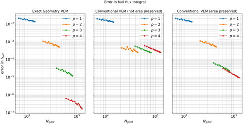
Figure 20. Convergence plots of $I_{\text{ab}1}$ for the exact-geometry VEM (left), the non-area-preserved classical VEM (middle) and area-preserved classical VEM (right).

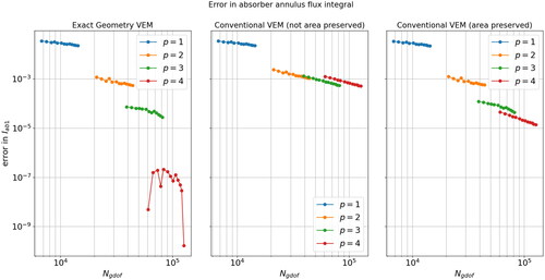
Figure 21. Convergence plots of $I_{\text{ab}2}$ for the exact-geometry VEM (left), the non-area-preserved classical VEM (middle) and area-preserved classical VEM (right).

Area preservation in the mesh refers to a process whereby the edges which approximate curves in linear meshes are pushed outward along the curve normals to correct the surface areas of each material subdomain. Section A.3 in the appendix provides more information on the area-preservation process.

For each QoI presented in Figures 18–21, the y-axis is shared between all three plots to facilitate easy comparison. The exact-geometry VEM result are the shown in the left images, the non-area-preserved linear mesh (middle) and the area-preserved linear mesh on the right.

From Figures 18–21, we may observe a few things:

• First, the exact geometry meshes exhibit superior convergence to the both linear meshes. The p = 3, 4 curves are shifted downward considerably and have a steeper slope. This indicates that the geometry error is not the dominant source of error and that the approximation error of the global VEM basis is the dominant source of error. As evidenced by the fact that by increasing the VEM order we both reduce the nominal value of the approximation error and increase the rate of convergence under h-refinement.

• Second, the non-area-preserved set of linear meshes exhibit sub-optimal convergence, with the observed order of convergence saturating at second-order. This implies that the limiting factor in the rate of convergence is the geometric error. Specifically, the rate at which the area of each material subdomains converge to those of the exact geometry.

• Third, the area-preserved set of linear meshes also exhibit sub-optimal convergence however the observed order of accuracy saturates at third-order. So, when compared to the non-area-preserved meshes, this scheme gains an order of accuracy. This is to be expected as the limiting factor in the geometric error is no longer the rate of convergence of the material subdomain areas to those of the exact geometry, but rather the rate of convergence of material interface arc-lengths to those of the exact geometry. If the arc-lengths between materials are wrong, then even if the areas of the material subdomains are correct, quantities such as neutron leakage between domains will be inaccurate.

The QoI which departs from this pattern is the flux integral over the burnable absorber pin $I_{ab2}.$ The non-area preserved meshes still exhibit considerable loss in accuracy however the area-preserved meshes do not. A possible explanation is that the scalar neutron flux field in the vicinity of the the burnable pin cell almost zero (see Figure 17). Under these conditions it is possible that for the area-preserved linear mesh, the geometric error is less significant and approximation error is more significant, thus leading to the situation where there is not much difference between the area-preserved linear mesh and the curvilinear mesh with respect to the value of $I_{\text{ab}2}.$

Alternatives to the NECG-VEM would include higher-order isoparametric FEM, where the description of element geometry uses the same finite element basis functions as the finite element itself. This means that elements have a piece-wise polynomial description of geometry. While superior to linear elements, this description of geometry is still unable to exactly represent conic sections such as circles and ellipses. Consequently, there will still be a geometric error associated with these schemes. In a series of papers on the application of Isogeometric Analysis (IGA) to neutron diffusion and neutron transport (Owens et al. 2016; Owens et al. 2017b; Owens et al. 2017c; Welch et al. 2017a; Welch et al. 2017b) the authors found that isoparametric FEM would also exhibit sub-optimal convergence rates in problems with curvilinear domains, for the same reasons the straight-sided VEM exhibited sub-optimal convergence.

6.4. The 2D OECD-NEA C5G7 benchmark verification test case

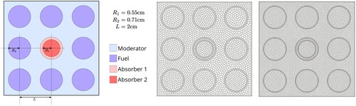
The 2D OECD-NEA C5G7 Benchmark verification test case, presented in (Lewis et al. 2003), is a nuclear reactor physics problem defined on a PWR geometry. The benchmark was developed in order to verify the ability of nuclear reactor physics codes to solve problems without spatial homogenization. The geometry of the problem is presented in Figure 22.

Figure 22. The geometry of the 2D C5G7 benchmark verification test case.

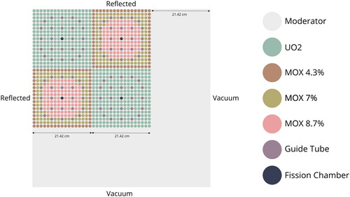
Symmetry along the x and y axes have reduced the problem to a quarter-core geometry consisting of two UOX assemblies and two MOX assemblies. Each assembly is a 17 × 17 array of nuclear fuel pins surrounded by a water reflector and each nuclear fuel pin has a radius of 0.54 cm. The values of the macroscopic nuclear cross section material data may be found in the OECD/NEA benchmark specification (Lewis et al. 2003).

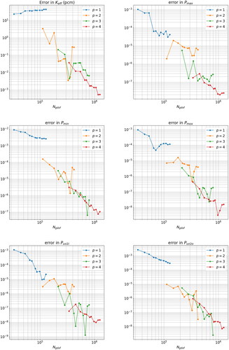
The quantities of interest (QoIs) are the the ${\mathrm{K}}_{\text{eff}},$ the maximum pin power $P_{\text{min}},$ the minimum pin power $P_{\text{min}},$ the power of either MOX assembly $P_{\text{MOX}},$ the power of the inner UO₂ assembly $P_{\text{UO}2\mathrm{i}}$ and the power of the outer UO₂ assembly $P_{\text{UO}2\mathrm{o}}.$ The full mathematical definitions of these QoIs are in the appendix (Figure 23). A reference solution was calculated using the VEM with a 129,802-element polygonal mesh and an order of p = 4. This reference solution had 2,028,163 DoFs per group. The values of the QoIs for this reference solution are given in Table 6.

Figure 23. Two examples of C5G7 curvilinear polygonal meshes.

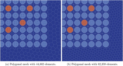
Table 6. Reference results for the C5G7 (2,028,163 DoFs).

${\mathrm{K}}_{\text{eff}}$	$P_{\text{max}}$	$P_{\text{min}}$	$P_{\text{MOX}}$	$P_{\text{UO}2\mathrm{o}}$	$P_{\text{UO}2\mathrm{o}}$
1.18324062	2.52089853	0.24063658	210.82158394	495.45445506	138.90237681

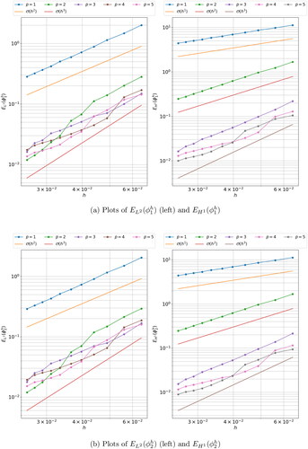
These values are in good agreement with the values presented in (Welch et al. 2017a), where a high-fidelity and exact-geometry IGA solution was calculated. The scalar neutron flux contours of the reference solution are given in Figure 24 for the $g=1,3,5,7$ energy groups. To investigate the numerical behavior of the exact-geometry VEM, the C5G7 was solved using a series of 10 polygonal meshes ranging from 22,968 elements to 82,359 elements and for orders $k=1,2,3,4.$ The QoIs were calculated for each mesh-order pair and the relative errors with respect to the reference values of Table 6 were computed. These errors are plotted in Figure 25. The convergence criterium used to terminate the power iteration was that given in Equation (3.38); the maximum relative difference between successive iterates of the scalar neutron flux. The tolerance for this criterium was set to $1\times {10}^{-12},$ at this value the C5G7 would require around 137 power iterations to converge. The scalar neutron fluxes were then normalized such that the fission source is equal to the number of nuclear fuel pins: 1056 (Lewis et al. 2003). $${\int }_V\sum _{g=1}^G\nu {\Sigma }_f^g{\varphi }_g(\mathit{x})dx=1056.$$

Figure 24. Scalar neutron flux contours for energy groups 1, 3, 5 and 7.

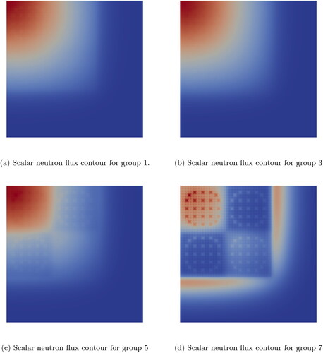
Figure 25. Errors in QoIs for the C5G7.

Figure 23a and b shows a portion of the 44,802 element mesh and the 82,359 element mesh from which the uniform refinement strategy may be seen. No adaptive refinement was used, additional elements were simply added to each region in proportion the surface area of each region.

Looking at the convergence curves of Figure 25 it is clear that for p = 2, 3, 4 there is a considerable amount of numerical noise. Particularly for p = 2, 3, the errors jump considerably. The reason for this is that the errors change sign, making the absolute value of the error appear to jump. However, it is still clear that the higher order curves are shifted downward relative to lower order curves and the errors themselves become very small, showing good agreement with the reference solution.

An additional complication is that the QoIs are a mix of global quantities, such as the ${\mathrm{K}}_{\text{eff}},$ and more localized quantities such as the min/max pin powers. Therefore, their error curves will exhibit different convergence properties depending upon how well converged the flux field is in the vicinity of the QoI. This is as problem that will be overcome in the future with adaptive mesh refinement (AMR) techniques which for each region of the nuclear reactor will converge the scalar neutron flux to roughly the same tolerance (Figure 26).

Figure 26. The control points of the bounding NURBS curves.

7. Conclusion

This paper presented the NURBS-enhanced VEM (NE-VEM) for the solution of the multigroup neutron diffusion equation (NDE). It extends the research presented in (Ferguson, Kópházi, and Eaton 2021) and addresses the main disadvantage of VEM presented in that paper: which was the geometric discretization error incurred by the use of straight-sided polygons to model curvilinear nuclear reactor geometries. The extension of the VEM to curvilinear polygons with NURBS edges eliminated the geometric discretization error from the lowest level of mesh refinement. As a consequence, the convergence curves for higher-order VEM schemes (p = 3, 4) show a marked improvement over those of the conventional VEM for benchmark verification test cases with curvilinear domains. This effect is demonstrated for a variety of QoIs, such as the L² and H¹ errors, in Sections 6.2 and 6.3.

The NE-VEM of this paper is built on top of a description of topology and geometry which is well suited both to specifying the geometrical and computational domain of interest, such as a nuclear reactor core, and for representing curvilinear, polygonal meshes. Therefore, under this regime, the distinction between what are usually known as the “domain” and the “mesh” has been eliminated. A benefit of this representation of topology/geometry over that of say isogeometric analysis (IGA) is that only those polygons which are incident on curvilinear boundaries or internal interfaces need be modeled using a NURBS boundary representation. While in IGA usually all of the elements are curvilinear to some extent as a consequence of the NURBS patch mapping from parametric space to the physical domain.

Additionally, we presented a method of integrating the scaled monomials up to a given order on curvilinear polygons. This method, Lassere’s Method, is very computationally efficient compared to direct quadrature and greatly reduces the time to compute local bilinear forms. Additionally, for the integration of functions which are not homogeneous, we presented a method of generating quadrature rules on curvilinear polygons using a subtessellation algorithm with Coons patches. We present our subtessellation method as an alternative to the quadrature rule algorithm presented in (Beirão da Veiga, Russo, and Vacca 2019). However our method requires the bounding curves of the polygon to be NURBS, while the method of (Beirão da Veiga, Russo, and Vacca 2019) does not.

The primary limitation of the work presented in this paper is the lack of adaptive hp refinement. In each of the benchmark verification test cases we presented the mesh sequences were uniformly refined. For the purposes of investigating the convergence rates of QoIs within nuclear reactor physics benchmark verification test cases this is acceptable. However, for large industrial nuclear reactor physics problems, where computational efficiency is paramount, this will be the limiting factor. Therefore, the implementation of common refinement strategies for the NDE, such as those presented in (Wang and Ragusa 2009; Wang, Bangerth, and Ragusa 2009), and methods of transferring solution fields between meshes, is a priority if the VEM is to have applications outside of academia. Another limitation of the work presented in this paper is the lack of a formal proof of well-posedness and a priori error analysis, therefore a more theoretical analysis of the discretization presented in this paper is also a priority.

A logical next step from the research presented in this paper is to apply the NE-VEM to the first-order form of the neutron transport equation (NTE). The NE-VEM has a number of favorable properties for the discrete ordinate (S${}_{\mathrm{N}}$) sweep algorithm used to solve the NTE. This favorable property is that for curvilinear meshes only a small subset of the elements will be curvilinear in shape (e.g. boundaries and some internal interfaces). The remaining polygonal elements within the mesh can be straight-sided. This has important implications in that the number of cyclic dependencies, where downstream fluxes depend on upstream fluxes and vice versa, will be reduced when compared to say IGA, where all elements can be curvilinear (Owens et al. 2016; Owens et al. 2017b; Owens et al. 2017c).

Data Statement

In accordance with EP SRC funding requirements all supporting data used to create figures in this paper may be accessed at the following URL: https://doi.org/10.5281/zenodo.6795306.

Acknowledgment

Mr. J. Ferguson would like to acknowledge the Engineering and Physical Sciences Research Council (EPSRC) through the Doctoral Training Partnership (DTP) PhD scheme (EPSRC Grant No.: EP/R512540/1). Mr. J. Ferguson also acknowledges the industrial and financial support of Rolls-Royce. Dr. M.D. Eaton and Dr. J. Kópházi would like to thank the Engineering and Physical Sciences Research Council (EPSRC) for their support through the following grants: Adaptive Hierarchical Radiation Transport Methods to Meet Future Challenges in Reactor Physics (EPSRC Grant No.: EP/J002011/1) and RADIANT: A Parallel, Scalable, High Performance Radiation Transport Modelling and Simulation Framework for Reactor Physics, Nuclear Criticality Safety Assessment and Radiation Shielding Analyses (EPSRC Grant No.: EP/K503733/1). The authors would like to thank Mr. M. Harvey, who is the research computing services (RCS) manager, and his team at Imperial College London. Finally, the authors would like to thank the anonymous reviewers for their suggestions.

Appendix A

A.1. Integration on curvilinear faceted polygons

Algorithm 1: Algorithm for integrating all scaled monomials $m_i(\mathit{x})$ up to order p

1: Input: Order p and a polygon F

2: Output: Set of scaled monomial integrals on F, $I_p^F.$

3: Translate F by $-{\mathit{x}}_F$ to get $\widehat{F}$

4: $I_p^F\leftarrow \text{IntegrateAll}(p,\widehat{F})$

5: for α = 1 to n_p do

6:  $q\leftarrow$ order of $m_{\alpha }(\mathit{x})$

7:  $I_p^F[\alpha ]\leftarrow \frac{1}{h_F^q}{I}_p^F[\alpha ]$ ⊳ property 5.2

8: end for

Algorithm 2: Algorithm for integrating all monomials $u_i(\mathit{x})$ up to order p on face $\widehat{F}$

1: procedure IntegrateAll(p, F) ⊳ Lassere on face

2:  $I_p^F\leftarrow [0,\dots ,0]$ ⊳ Initialize integrals to zero

3:  for $e_i\in \partial F$ do ⊳ For each edge

4:   if e_i is a linear then

5:    $I_p^{e_i}\leftarrow \text{IntegrateAll}(p,e_i)$ ⊳ integrate all monomials on edge

6:   else

7:    $I_p^{e_i}\leftarrow [0,\dots ,0]$

8:    for α = 1 to n_p do

9:     Apply quadrature on curve: $$I_p^{e_i}\left[\alpha \right]\leftarrow \sum _{j=1}^{\text{nqp}}\mathbf{c}(t_j).\mathbf{n}(t_j)u_{\alpha }(\mathbf{c}(t_j))w_j|J(t_j)|$$

10:    end for

11:   end if

12:   for α = 1 to n_p do ⊳ Add contribution from edge e_i to face integral

13:    Let $({\alpha }_x,{\alpha }_y)$ be the exponents of $u_{\alpha }(\mathit{x})$

14:    Let $q={\alpha }_x+{\alpha }_y$ ⊳ Monomial order

15:    $I_p^F[\alpha ]\leftarrow I_p^F[\alpha ]+\frac{1}{2+q}{I}_p^{e_i}[\alpha ]$

16:   end for

17:  end for

18:  return $I_p^F$

19: end procedure

Algorithm 3: Algorithm for integrating all monomials $u_i(\mathit{x})$ up to order p on edge $e\in \partial \widehat{F}$

1: procedure IntegrateAll(p, e) ⊳ Lassere on edge

2:  $I_p^e\leftarrow [0,\dots ,0]$

3:  $I_p^{{\mathbf{v}}_{i,2}}\leftarrow \text{IntegrateAll}(p,{\mathbf{v}}_{i,2})$ ⊳ integrate on second vertex of edge

4:  for α = 1 to n_p do

5:   Let $({\alpha }_x,{\alpha }_y)$ be the exponents of $u_{\alpha }(\mathit{x})$

6:   Let $q={\alpha }_x+{\alpha }_y$ ⊳ Monomial order

7:   Let ${\beta }_1=\alpha ({\alpha }_x-1,{\alpha }_y)$ and ${\beta }_2=\alpha ({\alpha }_x,{\alpha }_y-1)$

8:   Apply quadrature on curve: $$I_p^e\left[\alpha \right]=\frac{1}{1+q}\left[\left|e\right|I_p^{{\mathbf{v}}_{i,2}}\left[\alpha \right]+{({\mathit{x}}_{0,i})}_1{\alpha }_x{I}_p^e\left[{\beta }_1\right]+{({\mathit{x}}_{0,i})}_2{\alpha }_y{I}_p^e\left[{\beta }_2\right]\right]$$

9:  end for

10:  return $I_p^e$

11: end procedure

Algorithm 4: Algorithm for integrating all monomials $u_i(\mathit{x})$ up to order p on vertex v.

1: procedure IntegrateAll(p, v) ⊳ Lassere on vertex

2:  $I_p^{\mathbf{v}}\leftarrow [0,\dots ,0]$

3:  for α = 1 to n_p do

4:   $I_p^{\mathbf{v}}[\alpha ]=u_{\alpha }(\mathbf{v})$

5:  end for

6:  return $I_p^{\mathbf{v}}$

7: end procedure

A.2. Quadrature comparison

This section shall present all supplementary data necessary to replicate the test case presented in Section 6.1. All the bounding curves of the test polygon have the following order, knot vector and control weights: $$p=2,\hspace{1em}\mathbf{u}=[0,0,0,1,1,1],\mathbf{w}=[1,1.5,1]$$ and the control points:

Table

Coordinate	${\mathbf{P}}_1$	${\mathbf{P}}_2$	${\mathbf{P}}_3$	${\mathbf{P}}_4$	${\mathbf{P}}_5$	${\mathbf{P}}_6$	${\mathbf{P}}_7$	${\mathbf{P}}_8$	${\mathbf{P}}_9$	${\mathbf{P}}_{10}$
x	0.0000e + 00	3.2322e-01	1.0000e + 00	7.5000e-01	1.0000e + 00	−5.0000e-01	−2.0000e + 00	−2.8232e + 00	−4.0000e + 00	−1.9393e + 00
y	0.0000e + 00	6.7677e-01	1.0000e + 00	2.0000e + 00	3.0000e + 00	2.7500e + 00	3.0000e + 00	1.8232e + 00	1.0000e + 00	7.4253e-01

A.3. Linear polygonal meshes and area preservation

In both the MMS test case and the burnable supercell test case we compare the NE-VEM to classical VEM. To perform this comparison we must use linear polygonal meshes for the classical VEM. There are two situations to consider: the first is where there has been no attempt to preserve the area of the mesh and the second is where the mesh has been altered so that surface areas of material subdomains are preserved between the geometric domain and the linear mesh. In the non-area-preserved case the vertex coordinates in the mesh are left unchanged and all higher-order NURBS curves in the mesh are converted to linear NURBS curves (this is the dashed blue line in Figure 27).

Figure 27. Illustration of the exact-geometry line segment (thick red arc), the non-area preserved linear approximation (dashed blue line) and area-preserved approximation (solid blue line).

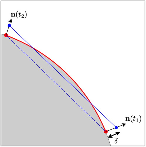
In the area-preserved case, we find all the vertices which lie on internal interface curves of the material subdomains and push them all outward by some distance δ along the outward normals of the pincell at each curve parameter (shown as $\mathbf{n}(t_1)$ and $\mathbf{n}(t_2)$ in Figure 27). The optimal offset distance δ is determined as follows: first the set of vertices in the original curvilinear mesh which lie incident with the boundary of the material subdomain are found, let us denote this set ${\left\{{\mathbf{v}}_i=(x_i,y_i)\right\}}_{i=1}^N$ and let us assume it is ordered counter-clockwise around the outer boundary of material subdomain. The area of the polygon enclosed by this loop is given by: $$A_{\text{poly}}=\frac{1}{2}\sum _{i=1}^N{x}_i{y}_{i+1}-x_{i+1}{y}_i,\hspace{1em}\text{where}\hspace{1em}(x_{N+1},y_{N+1})=(x_0,y_0)$$

Next, we compute the outward normal ${\mathbf{n}}_i=(n_{i,x},n_{i,y})$ to the pincell boundary at each point ${\mathbf{v}}_i.$ Let us assume the material subdomain has area A, then the offset distance δ is computed as a minimization problem: $$\delta =\arg \underset{\delta \in {\mathbb{R}}^{+}}{\min }{\left(A-\frac{1}{2}\sum _{i=1}^{N+1}(x_i+\delta n_{i,x})(y_{i+1}+\delta n_{i+1,y})-(x_{i+1}+\delta n_{i+1,x})(y_i+\delta n_{i,y})\right)}^2$$

Once the offset δ has been found each of the vertices ${\mathbf{v}}_i$ are displaced by $\delta {\mathbf{n}}_i.$ After this has been done, and all higher-order NURBS curves are replaced with linear NURBS curves between the newly computed vertices, the material subdomains of the linear mesh now have the same surface areas as the curvilinear mesh but are composed solely of linear elements.

A.4. Method of manufactured solutions

This section shall provide all the supplementary information needed to replicate the MMS benchmark verification test case of Section 6.2, beginning with the values of the macroscopic nuclear cross section material data are presented in Table 7.

Next, the construction of the forcing functions f₁ and f₂ shall be explained. Let $D_{V_1}^1=D^1{|}_{V_1}$ and $D_{V_2}^1=D^1{|}_{V_2},$ with the same subscript used for the other quantities to denote the same meaning. Let $d(\mathit{x}):{\mathbb{R}}^2\to {\mathbb{R}}^{}$ be the signed distance function of V₁, which is defined as: $$d(\mathit{x})=\text{sgn}(\mathit{x}){\min }_{\mathbf{y}\in \partial V_1}{\Vert \mathit{x}-\mathbf{y}\Vert }_{{\mathbb{R}}^2},\hspace{1em}\text{where}\hspace{1em}\text{sgn}(\mathit{x})=\{\begin{array}{c}-1\hspace{1em}\text{if}\hspace{1em}\mathit{x}\in V_1\hfill \\ 1\hspace{1em}\text{otherwise}\hfill \end{array}.$$

The distance function has two important properties which also provide useful information. First, for $\mathit{x}\in V_1$ the gradient $\nabla d(\mathit{x})$ points in the direction of the closest point on $\partial V_1,$ denoted y. Second, provided x is not equidistant to more than one point on $\partial V_1,$ that $\nabla d(\mathit{x})$ is equal to the outward normal vector at the nearest point y, this normal vector shall be denoted $\mathbf{n}(\mathit{x}).$ An example is presented in Figure 28.

Figure 28. On the left are the isolines of $d(\mathit{x}),$ on the right is an illustration of the properties of $\nabla d(\mathit{x})$ for $\mathit{x}\in V_1.$

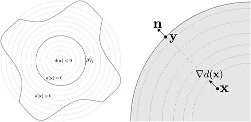
Computing the signed distance function of a general curve is a non-trivial task typically accomplished by solving the Eikonal equation, ${\Vert \nabla d\Vert }_{{\mathbb{R}}^2}=1,$ using fast marching methods. A survey of which may be found in (Sethian 1999). However, because the boundary curve $\partial V_1$ in the present test case is a circle of radius R = 3 and center (0, 0), albeit in NURBS form, the distance function has a simple expression. Letting $\mathit{x}=(x_1,x_2),$ the distance function may be written as: $$d(\mathit{x})=\sqrt{x_1^2+x_2^2}-R$$

Therefore, all of the physical quantities may be written in the same way as D¹ is below: $$D^1(\mathit{x})=D_{V1}^1+\left(D_{V2}^1-D_{V1}^1\right)H(d(\mathit{x}))=D_{V1}^1+\left[\mathrm{}\right[D^1\left]\mathrm{}\right]H(d(\mathit{x})),$$ where $H(t):{\mathbb{R}}^{}\to {\mathbb{R}}^{}$ is the Heaviside step function and $[\mathrm{}[D^1]\mathrm{}]$ denotes the jump in D¹ across the discontinuity. Substituting this description of the physical quantities and the manufactured solutions, ${\widehat{\varphi }}_1,{\widehat{\varphi }}_2,$ into Equation (6.2)(6.2) $$\{\begin{array}{c}\text{Find}\mathrm{ }\varphi \in {\left[H^1\left(V\right)\right]}^2\text{such}\mathrm{ }\text{that}\\ A(v,\varphi )=l\left(v\right)\hspace{1em}\forall v\in {\left[H^1\left(V\right)\right]}^2\end{array},$$(6.2) to gives: $$\begin{array}{c}{f}_1=-\nabla .\left(D^1\nabla \widehat{{\varphi }_1}\right)+{\Sigma }_r^1\widehat{{\varphi }_1}\\ f_2=-\nabla .\left(D^2\nabla \widehat{{\varphi }_2}\right)+{\Sigma }_r^2\widehat{{\varphi }_2}-{\Sigma }_s^{1\to 2}{\widehat{\varphi }}_1.\end{array}$$

Therefore, the source functions are piecewise continuous with a discontinuity at $\partial V_1.$ The diffusion terms require some further explanation as they include derivatives of discontinuous functions, beginning with the diffusion term for ${\widehat{\varphi }}_1:$ $$\begin{array}{c}-\nabla .\left(D^1\nabla \widehat{{\varphi }_1}\right)=-\nabla .\left(\left(D_{V1}^1+\left[\mathrm{}\right[D^1\left]\mathrm{}\right]H(d(\mathit{x}))\right)\nabla \widehat{{\varphi }_1}\right)\\ =-\nabla .\left(D_{V_1}^1\nabla {\widehat{\varphi }}_1\right)-\nabla .\left(\left[\mathrm{}\right[D^1\left]\mathrm{}\right]H(d(\mathit{x}))\nabla {\widehat{\varphi }}_1\right)\\ =\underset{\text{term}\mathrm{ }1}{\underbrace{-\left(D_{V_1}^1+\left[\mathrm{}\right[D^1\left]\mathrm{}\right]H(d(\mathit{x}))\right){\nabla }^2{\widehat{\varphi }}_1}}-\underset{\text{term}\mathrm{ }2}{\underbrace{\left[\mathrm{}\right[D^1\left]\mathrm{}\right]\nabla H(d(\mathit{x})).\nabla {\widehat{\varphi }}_1}}.\end{array}$$

Term 1 is a volume source, defined for all V, and may be written as: $$-\left(D_{V_1}^1+\left[\mathrm{}\right[D^1\left]\mathrm{}\right]H(d(\mathit{x}))\right){\nabla }^2{\widehat{\varphi }}_1=\{\begin{array}{c}-D_{V_1}^1{\nabla }^2{\widehat{\varphi }}_1\hspace{1em}\text{if}\hspace{1em}\mathit{x}\in V_1\hfill \\ -D_{V_2}^1{\nabla }^2{\widehat{\varphi }}_1\hspace{1em}\text{if}\hspace{1em}\mathit{x}\in V_2\hfill \end{array}.$$

Term 2 is a line source, defined only on $\partial V_1,$ and is computed as follows. Beginning with the $\nabla H(d(\mathit{x}))$ term: $$\frac{\partial }{\partial x_i}H(d(\mathit{x}))=\frac{\partial H(d(\mathit{x}))}{\partial d(\mathit{x})}.\frac{\partial d(\mathit{x})}{\partial x_i}=\delta (d(\mathit{x}))\frac{\partial d(\mathit{x})}{\partial x_i},$$ where $\delta (t)$ is the Dirac delta distribution. Therefore, $\nabla H(d(\mathit{x}))=\delta (d(\mathit{x}))\nabla d(\mathit{x}).$ Substituting this back into term 2 gives: $$\left[\mathrm{}\right[D^1\left]\mathrm{}\right]\nabla H(d(\mathit{x})).\nabla {\widehat{\varphi }}_1=\left[\mathrm{}\right[D^1\left]\mathrm{}\right]\left(\delta (d(\mathit{x}))\nabla d(\mathit{x})\right).\nabla {\widehat{\varphi }}_1$$

The same result can be reached for the group 2 diffusion term, $-\nabla .(D^2\nabla \widehat{{\varphi }_2}),$ using the same argument.

To see how the forcing linear forms are computed in practice, consider the forcing term: $$\begin{array}{c}{\left(v_1,f_1\right)}_{0,V}={\left(v_1,-\nabla .\left(D^1\nabla \widehat{{\varphi }_1}\right)+{\Sigma }_r^1\widehat{{\varphi }_1}\right)}_{0,V}\\ =-{\left(v_1,D_{V_1}^1{\nabla }^2{\widehat{\varphi }}_1\right)}_{0,V_1}-{\left(v_1,D_{V_2}^1{\nabla }^2{\widehat{\varphi }}_1\right)}_{0,V_2}+\left[\mathrm{}\right[D^1\left]\mathrm{}\right]{\left(v_1,{\mathbf{n}}_1.\nabla {\widehat{\varphi }}_1\right)}_{0,\partial V_1}+{\left(v_1,{\Sigma }_r^1{\widehat{\varphi }}_1\right)}_{0,V}\end{array}$$

Where ${\mathbf{n}}_1(\mathit{x})=\nabla d(\mathit{x}),\mathit{x}\in \partial V_1,$ is the outward normal to $\partial V_1.$ This is a property of the distance function which was explained earlier.

References

- Ahmad, B., A. Alsaedi, F. Brezzi, L. Marini, and A. Russo. 2013. Equivalent projectors for virtual element methods. Comput. Math. Appl. 66 (3):376–91. doi:10.1016/j.camwa.2013.05.015
- Aigner, M., C. Heinrich, B. Jüttler, E. Pilgerstorfer, B. Simeon, and A. V. Vuong. 2009. Swept volume parameterization for isogeometric analysis. In Mathematics of Surfaces XIII. Mathematics of Surfaces 2009. Lecture Notes in Computer Science, vol. 5654, 19–44. Berlin, Heidelberg: Springer. doi:10.1007/978-3-642-03596-8_2
- Antonietti, P. F., G. Manzini, and M. Verani. 2018. The fully nonconforming virtual element method for biharmonic problems. Math. Models Methods Appl. Sci. 28 (2):387–407. doi:10.1142/S0218202518500100
- Antonietti, P. F., P. Houston, and G. Pennesi. 2018. Fast numerical integration on polytopic meshes with applications to discontinuous Galerkin finite element methods. J. Sci. Comput. 77 (3):1339–70. doi:10.1007/s10915-018-0802-y
- Ayuso de Dios, B., K. Lipnikov, and G. Manzini. 2016. The nonconforming virtual element method. ESAIM: M2AN 50 (3):879–904. doi:10.1051/m2an/2015090
- Balay, S., S. Anhyankar, M. F. Adams, J. Brown, P. Brune, D. Buschleman, D. Kaushik, M. G. Knepley, D. A. May, L. C. McInnes, et al. 2020. PETSc users’ manual. Tech. rep., Argonne National Laboratory, Lemont, IL.
- Bazilevs, Y., V. Calo, J. Cottrell, J. Evans, T. Hughes, S. Lipton, M. Scott, and T. Sederberg. 2010. Isogeometric analysis using T-splines. Comput. Methods Appl. Mech. Engng. 199 (5-8):229–63. doi:10.1016/j.cma.2009.02.036
- Beall, M. W., and M. S. Shephard. 1997. General topology-based mesh data structure. Int. J. Numer. Meth. Engng. 40 (9):1573–96. doi:10.1002/(SICI)1097-0207(19970515)40:9¡1573::AID-NME128¿3.0.CO;2-9
- Beirão da Veiga, L., A. Russo, and G. Vacca. 2019. The virtual element method with curved edges. ESAIM: M2AN 53 (2):375–404. doi:10.1051/m2an/2018052
- Beirão da Veiga, L., F. Brezzi, A. Cangiani, G. Manzini, L. D. Marini, and A. Russo. 2013. Basic principles of virtual element methods. Math. Models Methods Appl. Sci. 23 (1):199–214. doi:10.1142/S0218202512500492
- Beirão da Veiga, L., F. Brezzi, L. D. Marini, and A. Russo. 2014. The Hitchhiker’s guide to the virtual element method. Math. Models Methods Appl. Sci. 24 (8):1541–73. doi:10.1142/S021820251440003X
- Beirão da Veiga, L., F. Brezzi, L. D. Marini, and A. Russo. 2016a. Virtual element method for general second-order elliptic problems on polygonal meshes. Math. Models Methods Appl. Sci. 26 (4):729–50. doi:10.1142/S0218202516500160
- Beirão da Veiga, L., F. Brezzi, L. D. Marini, and A. Russo. 2016b. Serendipity nodal VEM spaces. Comput. Fluids 141:2–12. doi:10.1016/j.compfluid.2016.02.015
- Beirão da Veiga, L., F. Brezzi, L. D. Marini, and A. Russo. 2020. Polynomial preserving virtual elements with curved edges. Math. Models Methods Appl. Sci. 30 (8):1555–90. doi:10.1142/S0218202520500311
- Berrone, S., A. Borio, and G. Manzini. 2018. SUPG stabilization for the nonconforming virtual element method for advection-diffusion-reaction equations. Comput. Methods Appl. Mech. Engng. 340:500–29. doi:10.1016/j.cma.2018.05.027
- Berrone, S., and A. Borio. 2017. Orthogonal polynomials in badly shaped polygonal elements for the Virtual Element Method. Finite Elem. Anal. Des. 129:14–31. doi:10.1016/j.finel.2017.01.006
- Bertoluzza, S., M. Pennacchio, and D. Prada. 2019. High order VEM on curved domains. Atti. Accad. Naz. Lincei Cl. Sci. Fis. Mat. Natur. 30 (2):391–412. doi:10.4171/RLM/853
- Biswas, R., and R. C. Strawn. 1994. A new procedure for dynamic adaption of three-dimensional unstructured grids. Appl. Numer. Math. 13 (6):437–52. doi:10.1016/0168-9274(94)90007-8
- Brenner, S. C., and L.-Y. Sung. 2018. Virtual element methods on meshes with small edges or faces. Math. Models Methods Appl. Sci. 28 (7):1291–336. doi:10.1142/S0218202518500355
- Brenner, S. C., Q. Guan, and L.-Y. Sung. 2017. Some estimates for virtual element methods. Comput. Methods Appl. Math. 17 (4):553–74. doi:10.1515/cmam-2017-0008
- Brezzi, F., and L. D. Marini. 2013. Virtual element methods for plate bending problems. Comput. Methods Appl. Mech. Engng. 253:455–62. doi:10.1016/j.cma.2012.09.012
- Cangiani, A., G. Manzini, and O. J. Sutton. 2016. Conforming and nonconforming virtual element methods for elliptic problems. IMA J. Numer. Anal. 37 (3):drw036. doi:10.1093/imanum/drw036
- Chin, E. B., J. B. Lasserre, and N. Sukumar. 2015. Numerical integration of homogeneous functions on convex and nonconvex polygons and polyhedra. Comput. Mech. 56 (6):967–81. doi:10.1007/s00466-015-1213-7
- Ciarlet, P. G. 2002. The finite element method for elliptic problems. Philadelphia, PA: Society for Industrial and Applied Mathematics. doi:10.1137/1.9780898719208
- Collins, B., A. Godfrey, S. Stimpson, and S. Palmtag. 2020. Simulation of the BEAVRS benchmark using VERA. Ann. Nucl. Energy 145:107602. doi:10.1016/j.anucene.2020.107602
- Coons, S. A. 1967. MAC-TR-41: Surfaces for computer-aided design of space forms. Tech. rep., Massachusetts Institute of Technology, Cambridge, MA.
- Coons, S. A. 1974. Surface patches and B-spline curves. In Computer aided geometric design, 1–16. New York, NY: Elsevier. doi:10.1016/B978-0-12-079050-0.50006-0
- Cox, M. G. 1972. The numerical evaluation of B-splines. IMA J. Appl. Math. 10 (2):134–49. doi:10.1093/imamat/10.2.134
- da Veiga, L. B., and G. Manzini. 2014. A virtual element method with arbitrary regularity. IMA J. Numer. Anal. 34 (2):759–81. doi:10.1093/imanum/drt018
- da Veiga, L. B., C. Lovadina, and A. Russo. 2017. Stability analysis for the virtual element method. Math. Models Methods Appl. Sci. 27 (13):2557–94. doi:10.1142/S021820251750052X
- da Veiga, L. B., F. Brezzi, L. D. Marini, and A. Russo. 2016. Virtual element implementation for general elliptic equations. In Building bridges: Connections and challenges in modern approaches to numerical partial differential equations, 39–71. Berlin, Heidelberg: Springer International Publishing. doi:10.1007/978-3-319-41640-3_2
- Dassi, F., and L. Mascotto. 2018. Exploring high-order three dimensional virtual elements: Bases and stabilizations. Comput. Math. Appl. 75 (9):3379–401. doi:10.1016/j.camwa.2018.02.005
- de Berg, M., O. Cheong, M. van Kreveld, and M. Overmars. 2008. Computational geometry. Berlin, Heidelberg: Springer. doi:10.1007/978-3-540-77974-2
- de Boor, C. 1972. On calculating with B-splines. J. Approximat. Theory 6 (1):50–62. doi:10.1016/0021-9045(72)90080-9
- Duderstadt, J. J., and L. J. Hamilton. 1976. Nuclear reactor analysis. Hoboken, NJ: John Wiley & Sons, Inc.
- Ferguson, J., J. Kópházi, and M. D. Eaton. 2021. Virtual element methods for the spatial discretisation of the multigroup neutron diffusion equation on polygonal meshes with applications to nuclear reactor physics. Ann. Nucl. Energy 151:107884. doi:10.1016/j.anucene.2020.107884
- Gaston, D. R., C. J. Permann, J. W. Peterson, A. E. Slaughter, D. Andrš, Y. Wang, M. P. Short, D. M. Perez, M. R. Tonks, J. Ortensi, et al. 2015. Physics-based multiscale coupling for full core nuclear reactor simulation. Ann. Nucl. Energy 84:45–54. doi:10.1016/j.anucene.2014.09.060
- Habetler, G. J., and M. A. Martino. 1958. KAPL-1886: The multigroup diffusion equations of reactor physics. Tech. rep., Knolls Atomic Power Laboratory, Niskayuna, NY.
- Hall, S. K., M. D. Eaton, and M. M. R. Williams. 2012. The application of isogeometric analysis to the neutron diffusion equation for a pincell problem with an analytic benchmark. Ann. Nucl. Energy 49:160–9. doi:10.1016/j.anucene.2012.05.030
- Harmel, M., R. A. Sauer, and D. Bommes. 2017. Volumetric mesh generation from T-spline surface representations. Comput-Aided. Des. 82:13–28. doi:10.1016/j.cad.2016.07.017
- Hebert, A. 2020. Applied reactor physics. 3rd ed. Montréal, Canada: Presses internationales Polytechnique.
- Hughes, T., A. Reali, and G. Sangalli. 2010. Efficient quadrature for NURBS-based isogeometric analysis. Comput. Methods Appl. Mech. Engng. 199 (5–8):301–13. doi:10.1016/j.cma.2008.12.004
- Hughes, T., J. Cottrell, and Y. Bazilevs. 2005. Isogeometric analysis: CAD, finite elements, NURBS, exact geometry and mesh refinement. Comput. Methods Appl. Mech. Engng. 194 (39–41):4135–95. doi:10.1016/j.cma.2004.10.008
- Kallinderis, Y., and P. Vijayan. 1993. Adaptive refinement-coarsening scheme for three-dimensional unstructured meshes. AIAA J. 31 (8):1440–7. doi:10.2514/3.11793
- Kang, C. M., and K. F. Hansen. 1973. Finite Element Methods for Reactor Analysis. Nucl. Sci. Eng. 51 (4):456–95. doi:10.13182/NSE73-A23278
- Khamayseh, A., and B. Hamann. 1996. Elliptic grid generation using NURBS surfaces. Comput. Aided Geom. Des. 13 (4):369–86. doi:10.1016/0167-8396(95)00050-X
- Lasserre, J. B. 1998. Integration on a convex polytope. Proc. Amer. Math. Soc. 126 (8):2433–41. doi:10.1090/S0002-9939-98-04454-2
- Latimer, C., J. Kópházi, M. D. Eaton, and R. G. McClarren. 2020. A geometry conforming isogeometric method for the self-adjoint angular flux (SAAF) form of the neutron transport equation with a discrete ordinate (SN) angular discretisation. Ann. Nucl. Energy 136:107049. doi:10.1016/j.anucene.2019.107049
- Latimer, C., J. Kópházi, M. D. Eaton, and R. McClarren. 2020. A geometry conforming, isogeometric, weighted least squares (wls) method for the neutron transport equation with discrete ordinate (SN) angular discretisation. Prog. Nucl. Energy 121:103238. doi:10.1016/j.pnucene.2019.103238
- Latimer, C., J. Kópházi, M. D. Eaton, and R. McClarren. 2021. Spatial adaptivity of the SAAF and Weighted Least Squares (WLS) forms of the neutron transport equation using constraint based, locally refined, isogeometric analysis (IGA) with dual weighted residual (DWR) error measures. J. Comput. Phys. 426:109941. doi:10.1016/j.jcp.2020.109941
- Lawrence, R. 1986. Progress in nodal methods for the solution of the neutron diffusion and transport equations. Prog. Nucl. Energy 17 (3):271–301. doi:10.1016/0149-1970(86)90034-X
- Lewis, E. E., M. A. Smith, N. Tsoulfanidis, G. Palmiotti, T. A. Taiwo, and R. N. Blomquist. 2003. Benchmark on deterministic transport calculations without spatial homogenisation: A 2-D/3-D MOX fuel assembly benchmark. Tech. Rep. NEA/NSC/DOC(2003)16, Nuclear Energy Agency (NEA), Organisation for Economic Co-operation and Development.
- Lin, F., and W. Hewitt. 1994. Expressing Coons-Gordon surfaces as NURBS. Comput-Aided. Des. 26 (2):145–55. doi:10.1016/0010-4485(94)90035-3
- Lin, H., S. Jin, Q. Hu, and Z. Liu. 2015. Constructing B-spline solids from tetrahedral meshes for isogeometric analysis. Comput. Aided Geom. Des. 35–36:109–20. doi:10.1016/j.cagd.2015.03.013
- Liu, X., J. Li, and Z. Chen. 2017. A nonconforming virtual element method for the Stokes problem on general meshes. Comput. Methods Appl. Mech. Engng. 320:694–711. doi:10.1016/j.cma.2017.03.027
- Mäntylä, M. 1983. Topological analysis of polygon meshes. Comput-Aided. Des. 15 (4):228–34. doi:10.1016/0010-4485(83)90126-4
- Mantyla, M. 1984. A note on the modeling space of Euler operators. Comput. Vis. Graph. Image Process. 26 (1):45–60. doi:10.1016/0734-189X(84)90129-4
- Mantyla, M., and R. Sulonen. 1982. GWB: A solid modeler with Euler operators. IEEE Comput. Grap. Appl. 2 (7):17–31. doi:10.1109/MCG.1982.1674396
- Manzini, G., A. Cangiani, and O. Sutton. The conforming virtual element method for the convection-diffusion-reaction equation with variable coeffcients. Tech. rep., Los Alamos National Laboratory (LANL), Los Alamos, NM, oct. 2014. doi:10.2172/1159207
- Mascotto, L. 2018. Ill-conditioning in the virtual element method: Stabilizations and bases. Numer. Methods Part. Different. Eq. 34 (4):1258–81. doi:10.1002/num.22257
- Miller, W. F., and E. E. Lewis. 1993. Computational methods of neutron transport, 1st ed. La Grange Park, IL: American Nuclear Society.
- Muller, D., and F. Preparata. 1978. Finding the intersection of two convex polyhedra. Theoretic. Comput. Sci. 7 (2):217–36. doi:10.1016/0304-3975(78)90051-8
- Mylonakis, A., M. Varvayanni, N. Catsaros, P. Savva, and D. Grigoriadis. 2014. Multi-physics and multi-scale methods used in nuclear reactor analysis. Ann. Nucl. Energy 72:104–19. doi:10.1016/j.anucene.2014.05.002
- Owens, A., J. Kópházi, and M. D. Eaton. 2017a. Optimal trace inequality constants for interior penalty discontinuous Galerkin discretisations of elliptic operators using arbitrary elements with non-constant Jacobians. Comput. Phys. 350:847–70. doi:10.1016/j.jcp.2017.09.020
- Owens, A., J. Kópházi, J. Welch, and M. D. Eaton. 2017b. Energy dependent mesh adaptivity of discontinuous isogeometric discrete ordinate methods with dual weighted residual error estimators. Comput. Phys. 335:352–86. doi:10.1016/j.jcp.2017.01.035
- Owens, A., J. Welch, J. Kópházi, and M. D. Eaton. 2016. Discontinuous isogeometric analysis methods for the first-order form of the neutron transport equation with discrete ordinate (SN) angular discretisation. Comput. Phys. 315:501–35. doi:10.1016/j.jcp.2016.03.060
- Owens, A., J. Welch, J. Kópházi, and M. D. Eaton. 2017c. An adaptive, hanging-node, discontinuous isogeometric analysis method for the first-order form of the neutron transport equation with discrete ordinate (SN) angular discretisation. Comput. Methods Appl. Mech. Engng. 318:215–41. doi:10.1016/j.cma.2017.01.036
- Piegl, L., and W. Tiller. 1995. The NURBS book, Monographs in visual communications. Berlin, Heidelberg: Springer. doi:10.1007/978-3-642-97385-7
- Russo, A. 2016. On the choice of the internal degrees of freedom for the nodal virtual element method in two dimensions. Comput. Math. Appl. 72 (8):1968–76. doi:10.1016/j.camwa.2016.03.016
- Sanchez, R. 2009. Assembly homogenization techniques for core calculations. Prog. Nucl. Energy 51 (1):14–31. doi:10.1016/j.pnucene.2008.01.009
- Schmidt, R., R. Wüchner, and K.-U. Bletzinger. 2012. Isogeometric analysis of trimmed NURBS geometries. Comput. Methods Appl. Mech. Engng. 241–244:93–111. doi:10.1016/j.cma.2012.05.021
- Schneider, T., D. Panozzo, and X. Zhou. 2021. Isogeometric high order mesh generation. Comput. Methods Appl. Mech. Engng. 386:114104. doi:10.1016/j.cma.2021.114104
- Semenza, L. A., E. E. Lewis, and E. C. Rossow. 1972. The application of the finite element method to the multigroup neutron diffusion equation. Nucl. Sci. Eng. 47 (3):302–10. doi:10.13182/NSE72-A22416
- Sethian, J. A. 1999. Fast Marching Methods. SIAM Rev. 41 (2):199–235. doi:10.1137/S0036144598347059
- Sevilla, R., S. Fernández-Méndez, and A. Huerta. 2008. NURBS-enhanced finite element method (NEFEM). Int. J. Numer. Meth. Engng. 76 (1):56–83. doi:10.1002/nme.2311
- Sevilla, R., S. Fernández-Méndez, and A. Huerta. 2011. 3D NURBS-enhanced finite element method (NEFEM). Int. J. Numer. Meth. Engng. 88 (2):103–25. doi:10.1002/nme.3164
- Smith, K. S. 1986. Assembly homogenization techniques for light water reactor analysis. Prog. Nucl. Energy 17 (3):303–35. doi:10.1016/0149-1970(86)90035-1
- Smith, K. S. 2017. Nodal diffusion methods and lattice physics data in LWR analyses: Understanding numerous subtle details. Prog. Nucl. Energy 101:360–9. doi:10.1016/j.pnucene.2017.06.013
- Sommariva, A., and M. Vianello. 2007. Product Gauss cubature over polygons based on Green’s integration formula. Bit Numer. Math. 47 (2):441–53. doi:10.1007/s10543-007-0131-2
- Stimpson, S., K. Clarno, R. Pawlowski, R. Gardner, J. Powers, B. Collins, A. Toth, S. Novascone, S. Pitts, J. Hales, et al. 2020. Coupled fuel performance calculations in VERA and demonstration on Watts Bar unit 1, cycle 1. Ann. Nucl. Energy 145:107554. doi:10.1016/j.anucene.2020.107554
- Wachspress, E. 1966. Iterative solution of elliptic systems and applications to the neutron diffusion equations of reactor physics. Hoboken, NJ: Prentice-Hall.
- Wang, Y., and J. Ragusa. 2009. Application of HP adaptivity to the multigroup diffusion equations. Nucl. Sci. Eng. 161 (1):22–48. doi:10.13182/NSE161-22
- Wang, Y., W. Bangerth, and J. Ragusa. 2009. Three-dimensional h-adaptivity for the multigroup neutron diffusion equations. Prog. Nucl. Energy 51 (3):543–55. doi:10.1016/j.pnucene.2008.11.005
- Welch, J., J. Kópházi, A. Owens, and M. D. Eaton. 2017a. A geometry preserving, conservative, mesh-to-mesh isogeometric interpolation algorithm for spatial adaptivity of the multigroup, second-order even-parity form of the neutron transport equation. J. Comput. Phys. 347:129–46. doi:10.1016/j.jcp.2017.06.015
- Welch, J., J. Kópházi, A. Owens, and M. D. Eaton. 2017b. Isogeometric analysis for the multigroup neutron diffusion equation with applications in reactor physics. Ann. Nucl. Energy 101:465–80. doi:10.1016/j.anucene.2016.11.015
- Wood, J., and M. M. R. Williams. 1984. Recent progress in the application of the finite element method to the neutron transport equation. Prog. Nucl. Energy 14 (1):21–40. doi:10.1016/0149-1970(84)90010-6
- Xu, G., B. Mourrain, R. Duvigneau, and A. Galligo. 2013a. Analysis-suitable volume parameterization of multi-block computational domain in isogeometric applications. Comput-Aided. Des. 45 (2):395–404. doi:10.1016/j.cad.2012.10.022
- Xu, G., B. Mourrain, R. Duvigneau, and A. Galligo. 2013b. Constructing analysis-suitable parameterization of computational domain from CAD boundary by variational harmonic method. Comput. Phys. 252:275–89. doi:10.1016/j.jcp.2013.06.029