Analyzing power and energy flexibilities by demand response in district heated buildings in Finland and Germany

Abstract

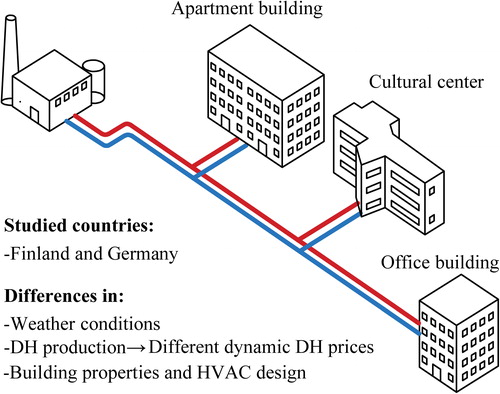
This study aims to investigate the effect of demand response (DR) on power and energy flexibilities with three types of district heated buildings (apartment building, cultural center, and office building) in Finland and Germany. A rule-based control algorithm was applied for the DR control with two country-specific dynamic district heating (DH) prices, the more fluctuating Finnish synthetic DH price and the flatter German synthetic DH price. This research was implemented with the validated dynamic building simulation tool IDA ICE. Set-point smoothing of the indoor air temperature was applied to minimize the rebound effect. Nighttime set-back was adopted in the cultural center and the office building. The results show that the DR control without smoothing creates additional peaks in power demand, while the set-point smoothing significantly decreases the peak power demand. The DR control can significantly shape the heating power demand of the buildings and increase energy flexibility. The range of the resultant seasonal energy flexibility factors is from 3 to 26% for charging and from −6 to −31% for discharging, depending on the building types and countries. Cases with nighttime set-back have higher power and energy flexibilities, while this causes additional peaks, which is detrimental to DH systems.

Introduction

The European Commission aims to achieve the key targets of cutting 40% of greenhouse gas emissions from 1990 levels, increasing the share of renewable energy by 32%, and improving energy efficiency at least 32.5% by 2030 (European Commission 2018). Moreover, the European Commission has a vision of being climate neutral by 2050 (European Commission 2020). Finland and Germany have also set the same ambitious climate target for reducing greenhouse gas emissions at least 55% by 2030 compared to the 1990 level (Finnish Government 2019; BMU 2019). In 2016, district heating (DH) totaled 33% of energy consumption in Finland (IEA 2018). Power and heat generation accounted for 40% of the total CO₂ emissions (IEA 2018). In addition, Germany (together with Poland) remains the biggest market for DH in the European Union (EU) and the proportion of renewable energy in DH consumption in Germany was only 12% in 2017 (Euroheat & Power and Moczko 2019). These figures verify that DH is prevalent both in Finland and Germany, offering immense potential for realizing these targets.

Increasing the share of renewable energy reduces the use of fossil fuels effectively, thereby reducing CO₂ emissions. However, energy generated by renewable sources such as wind and solar power is intrinsically variable. The existing energy system may become unstable if the proportion of renewable sources increases on a large scale (Robert, Sisodia, and Gopalan 2018). Therefore, to accommodate this flexible energy system, thermal energy storage (TES) was introduced in both electricity and DH networks. The integration of TES into the DH network balances the heat supply and demand effectively, thereby decreasing the need for peak generation (Salo et al. 2019). In addition, energy consumption needs to be flexible.

For this purpose, an active method called demand response (DR) has been introduced. Dynamic energy price is applied as one of the incentives for prosumers (Miller and Senadeera 2017; Zafar et al. 2018) to store or share energy actively. Moreover, demand-side management techniques have been put forth to optimize production or reduce costs (Gelazanskas and Gamage 2014). Energy-flexible buildings were also allowed for demand-side management or load control according to user needs, local climate conditions, and grid requirements (Jensen et al. 2017).

At first, most of the research on energy flexibility investigated only the building level, while as research accumulated, more scholars began to analyze ways in which the flexibility of buildings affects energy supply systems and their flexibilities. However, there is no unified energy flexibility definition because as the research object changes, the definition also changes. Similarly, various methodologies have been proposed based on the definition of flexibility followed by the respective researchers. This resulted in the identification of three characteristics pertinent to the definition: cost saving potential, temporal flexibility, and the amplitude of energy or power modulation (Reynders et al. 2018).

The cost saving potential of DR has typically been examined based on the dynamic electricity price (Yoon, Baldick, and Novoselac 2016; Cai and Braun 2019). In a Danish study, a flexibility index for cost saving was proposed for analyzing the impact of changes in the proportion of wind, solar, and ramp energy with different dynamic electricity prices on building flexibility index (Junker et al. 2018). A cost curve was designed to illustrate a Belgium office function of cost saving rate and the amount of electricity that can be shifted compared with the case without DR control (De Coninck and Helsen 2016).

Temporal flexibility and the amplitude of energy or power modulation were defined mainly to quantify the flexibility potential of TES. This can be divided into two aspects. First, researchers investigated the impacts of thermal mass capacity on the energy flexibility of heated buildings or clusters. Reynders, Diriken, and Saelens (2017) proposed three quantification methods, available storage capacity, storage efficiency, and power-shifting capability, to quantify the active DR characteristics for the structural TES capacity for residential buildings. The available storage capacity denoted the amount of energy stored in the thermal mass within limited hours. Storage efficiency described the percentage of stored energy successfully emitted to the indoor air to maintain thermal comfort. Power shifting capability showed the relation between the change in heating power and the duration for which this shift was maintained. Furthermore, Le Dréau and Heiselberg (2016) and Johra, Heiselberg, and Le Dréau (2019) put forward two types of flexibility indexes that combined dynamic energy price and the amount of shifted energy to quantify the ability in residential buildings to minimize the heating energy usage when the price was high and maximize it when the price was low. Similarly, load shifting efficiency was presented to describe the share of stored thermal energy that was employed to decrease the consumption for peak consumption periods (Hedegaard et al. 2019). The study simulated 159 detached houses to analyze the relationship between charging and discharging energies of thermal mass and energy price variations.

In addition, researchers proposed flexibility factors mainly to quantify ways in which a storage system provides flexible operation to an electricity or a heating system. Nuytten et al. (2013) defined delayed and forced operation flexibility indexes to quantify the hours that a combined heat and power (CHP) system can remain off or the hours needed by a TES system for charging. It was indicated that the water tank size had an almost linear influence on the flexibility of the CHP system. Furthermore, power shifting potential was proposed as the maximum shifted power deviated from the reference case (Oldewurtel et al. 2013). Moreover, power shifting efficiency was defined as the ratio of power shifting potential to energy consumption difference of the simulation period. It was shown that the power shifting potential and power shifting efficiency varied by the hour of the day and weather conditions through a heat pump system simulation. Stinner, Huchtemann, and Müller (2016) developed three types of flexibility factors, temporal flexibility, power flexibility, and energy flexibility, to analyze the flexibility potential of TES in a building energy system. Delayed and forced operational flexibility factors were defined similarly to what has been already described before. Power flexibility factors were defined as average delayed and forced power flexibilities to describe average discharging and charging power during temporal flexibility periods of TES. Energy flexibility factors were defined as delayed and forced energy flexibilities to describe the maximum discharging or charging energy of TES.

The research on flexibility factors is mainly addressing cost, time, and power or energy. Although most studies are based on electricity price or electricity consumption, these factors can also apply to district heated buildings or systems. Moreover, control strategies for DR were another research area of district heated buildings or systems. A control strategy named domestic hot water prioritizing methodology has been developed that decreased by nearly 15% the power peaks in student apartment buildings (Ala-Kotila, Vainio, and Heinonen 2020). Salo et al. (2019) illustrated that heat production costs were decreased using optimal DR control strategies. Moreover, the centralized hot water storage tank enhanced the ability to use DR strategies for more cost savings. In addition, it was presented that demand-side management control strategies should be distinctively built for different customers and they decreased the annual peak heat load little without energy savings (Kontu et al. 2018).

However, the research just described mostly analyzed the flexibility of a single building type. Residential buildings and their clusters were the most popular. Only a few studies compared the flexibility of different types of buildings with various occupant schedules. Moreover, most papers investigated the flexibility of buildings with DR control based on dynamic electricity prices. Research is equally limited to the impact of different dynamic prices on flexibility. Therefore, analysis of the flexibility of different district heated building types is required with dynamic DH prices, and the comparison of different types of dynamic DH prices needs to be considered. Moreover, there are few papers that applied smoothing of indoor temperature set-point changes to prevent a sudden peak load increase, which is called a rebound effect (Palensky and Dietrich 2011; Shan et al. 2016).

This article investigates ways in which DR affects the power and energy flexibility of three types of district heated buildings from the perspective of DH producers. An apartment building, a cultural center, and an office building were simulated in both Finland and Germany. The novelty of this study is, first, that three types of buildings with different customer modes were simulated and analyzed, while previous research was restricted to one type of building and its occupants’ style. Second, instead of optimizing and comparing control strategies, the impacts of two different DH prices in Finland and Germany were compared under the same control strategy. Moreover, smoothing of indoor temperature set-point changes was applied to minimize the rebound effect, and for the cultural center and office building, the advantages and disadvantages of nighttime set-back were pointed out.

Methodology

Description of simulation process

Three types of buildings, an apartment building, a cultural center, and an office building, in both Finland and Germany were simulated, as shown in Figure 1. The buildings were simulated with Finnish and German weather conditions. In addition, two country-specific dynamic district heat prices were employed, the Finnish and German synthetic DH prices.

Fig. 1. General description of simulation study.

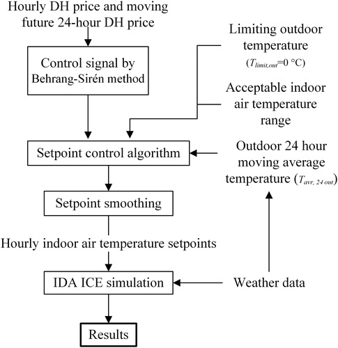
Figure 2 describes the simulation process. The Behrang–Sirén method (Alimohammadisagvand, Jokisalo, and Sirén 2018; Vand et al. 2020; Ju et al. 2021) changed the hourly DH price into control signals. Outdoor 24-hour moving average temperature, acceptable indoor air temperature range, and limiting outdoor temperature were employed in the set-point control algorithm. After that, set-point smoothing was adopted to prevent a sudden peak load increase, and final hourly indoor temperature set-points were obtained. Buildings were simulated by IDA ICE for results.

Fig. 2. Flow chart of simulation process.

Acceptable range of indoor air temperature set-points

The acceptable range of indoor air temperature set-points was defined based on the middle class S2 of the classification of indoor environment by the Finnish Society of Indoor Air Quality (2018). When the 24-h moving average outdoor temperature is below 0 °C, the operative temperature should keep within 20–23 °C. The minimum acceptable indoor air temperature was chosen according to the thermal environmental category II of standard EN 15251 (2007). Based on these, the acceptable indoor air temperature set-points for space heating were chosen to be from 20 °C to 23 °C for both the Finnish and German cases.

Hourly DH prices

Two country-specific DH prices were adopted: Finnish and German synthetic DH prices. Price fluctuation is caused by the variation of the district heating production costs, including CHP earnings. These synthetic DH prices describe the prices defined by the producer using a real-time pricing mechanism, which defines the prices according to the hourly fuel prices, also taking into account the profits from selling electricity by CHP units. More detailed information on the DH prices is available in Salo et al. (2019) and Suhonen et al. (2020). The Finnish synthetic DH price represents a typical district heat producer in Finland and contains both energy and transfer costs and a value-added tax of 24% (VAT). In this case, the typical DH system on the production side consists of a biomass-fired CHP plant and an oil-fired heat-only boiler. The German synthetic DH price was calculated based on the actual heat generation costs for a portfolio of heat generators currently operating in a district of Hamburg (biomethane CHP plants and natural gas boilers). Thereby, fuel price data were assumed to be 23,44 €/MWh for natural gas (Sandrock et al. 2016) and 64,00 €/MWh for biogas (Bundesnetzagentur 2014). The yearly average price is the same as the actual yearly DH price (including energy, transfer, and taxes) used in Hamburg by a DH company. Figure 3 depicts the Finnish and German synthetic real-time DH prices. In this analysis, it was assumed that district heating producers published 24-h DH prices ahead of time.

Fig. 3. Finnish and German synthetic DH prices.

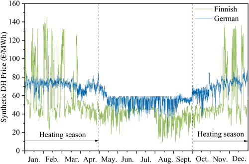
In this article, the months from January to April and from October to December were chosen for analysis because most of the heating demand occurred in these months. The same period was applied in both countries for consistency. The analyzed period is called the heating season in this article. The Finnish and German synthetic prices as average, maximum, minimum, and standard deviation for each month during the heating season are respectively shown in Tables 1 and 2. The Finnish price fluctuates significantly more during the coldest winter months. However, the fluctuation of the German price is quite stable during the whole heating season. Average values in March and April for the Finnish price are much lower than in other months. Conversely, the German price average values are quite similar each month. The maximum Finnish price is 145.4 €/MWh, while the German one is only 90.6 €/MWh.

Table 1. Description of the Finnish synthetic DH price.

Month	Average (€/MWh)	Maximum (€/MWh)	Minimum (€/MWh)	Standard deviation (€/MWh)
January	67.6	138.0	32.3	26.5
February	72.1	145.4	22.4	34.5
March	65.9	133.2	36.1	27.5
April	44.7	54.6	28.2	5.8
October	41.3	50.0	24.1	5.3
November	57.2	136.7	33.8	22.7
December	65.5	136.4	27.0	30.7
Heating season	59.1	145.4	22.4	26.7

Table 2. Description of the German synthetic DH price.

Month	Average (€/MWh)	Maximum (€/MWh)	Minimum (€/MWh)	Standard deviation (€/MWh)
January	72.1	84.1	48.5	5.7
February	74.0	83.6	64.1	3.2
March	71.3	80.6	56.9	4.2
April	68.7	84.6	53.9	5.1
October	62.9	84.6	35.5	6.3
November	70.6	82.3	47.4	5.7
December	75.5	90.6	61.9	4.6
Heating season	70.7	90.6	35.5	6.4

Weather data

For Finnish cases, buildings locate in Helsinki in Finnish climate zone I (Kalamees et al. 2012). Therefore, the heating systems of these buildings were dimensioned using the design outdoor temperature −26 °C, and simulations were carried out with hourly weather data for Helsinki–Vantaa, test reference year TRY2012 (Kalamees et al. 2012; FMI 2020). For German cases, buildings were located in Hamburg with a design outdoor temperature of −12 °C and hourly weather data of Hamburg, test reference year TRY2015 (DWD 2017, 2020). Table 3 shows the outdoor temperatures of these test reference years. During the heating season, the outdoor temperature of Helsinki is lower and fluctuates more than that of Hamburg. The average temperature of Helsinki during the heating season is −0.3 °C, while it is 5.2 °C in Hamburg. For Helsinki, February is the coldest month with an average temperature of −4.5 °C and a minimum temperature of −20.6 °C, and the minimum temperatures are quite similar in January, February, and March. For Hamburg, January is the coldest month with an average temperature of 1.8 °C and a minimum temperature of −9.4 °C. The number of heating degree days for Helsinki for an indoor air temperature of 17 °C is 3952 °C·d, while this is 2498 °C·d for Hamburg.

Table 3. Description of Helsinki and Hamburg outdoor temperatures of test reference years.

Month	Average (ºC)		Maximum (ºC)		Minimum (ºC)		Standard deviation (ºC)
	Finland	Germany	Finland	Germany	Finland	Germany	Finland	Germany
January	−4.0	1.8	2.8	9.5	−20.4	−9.4	5.7	3.6
February	−4.5	2.6	8	10.2	−20.6	−5	7.2	2.7
March	−2.6	5.1	6.2	19.5	−19.9	−5.2	4.6	4.0
April	4.5	9.0	18.3	19.6	−3.7	−1.5	4.6	4.2
October	6.2	9.9	13.9	17.5	−2.1	−0.4	3.6	3.8
November	0.5	5.7	8.9	15.1	−17.8	−4.6	6.3	4.7
December	−2.2	2.0	4.9	8.4	−15	−6	4.5	3.2
Heating season	−0.3	5.2	18.3	19.6	−20.6	−9.4	6.6	4.9

Building simulation tool

The building simulation tool IDA Indoor Climate and Energy (IDA ICE) version 4.8 was chosen for this study (Sahlin 1996). IDA ICE is a dynamic multizone simulation software program that provides a platform where users can model characteristics of a building and its technical systems such as building geometry and structures, HVAC systems, and user profiles. It was validated against the EN 15255-2007 and EN 15265-2007 standards (Equa Simulation 2010a). Also, it has been validated in several studies (Bring, Sahlin, and Vuolle 1999; Moosberger 2007; Equa Simulation 2010b), which provided strong justification for using IDA ICE in this article.

Description of building models

Three building types with different properties and designs of HVAC systems were selected to represent typical buildings in Finland and Germany. The buildings were simulated with normal Finnish or German design practices and weather conditions, while the geometry of the same building type was the same.

The German cultural center and office building were assumed to be built in 1980s and the apartment building in the 1930s, while all the simulated buildings in Finland were assumed to be built in 1990s. The German cultural center and office building have been renovated in recent years. Table 4 lists the basic model parameters of these three types of buildings.

Table 4. Building model parameters.

Parameters	Apartment building	Cultural center	Office building
Heated net floor area (m^2)	4885	3937	2383
Floor number	4	3	4
Envelope area (m^2)	4780	6921	3855
Window/envelope area	7.6%	8.8%	9.5%

Building structure

Table 5 shows the U values and air tightness of the buildings. In Finnish cases, these three types of buildings share the same parameters except for the air leakage rate. In German cases, the cultural center and the office building share the same parameters except for the air leakage rate. The load-bearing structures are mainly brick or concrete with a high thermal storage capacity, which can be well suited for the DR control of space heating.

Table 5. U values and airtightness of buildings.

Parameters		Finland			Germany
		Apartment building	Cultural center	Office building	Apartment building	Cultural center	Office building
U value (W/m^2·K)	External walls	0.28	0.28	0.28	1.70	0.20	0.20
	Roof	0.22	0.22	0.22	1.40	0.19	0.19
	Ground slab	0.36	0.36	0.36	1.00	0.28	0.28
	Windows	1.00	1.00	1.00	3.00	3.00	3.00
Air leakage rate, n50 (1/h)		1.00	2.00	1.60	7.00	3.00	4.50

Heating and ventilation system

All these simulated buildings are connected to the DH network. The water radiator systems were designed based on different outdoor temperatures because of different locations. Table 6 shows design powers of heating systems at different temperatures. The design temperatures are −26 and −12 °C, respectively, with a design indoor air temperature of 21 °C. Higher U values and air leakage rate for the German apartment building result in higher space heating design power. Figure 4 depicts control curves of different inlet water temperatures for the three types of buildings. There are mechanical cooling systems only in the Finnish cultural center and office building.

Fig. 4. Inlet water temperature adjustment in relation to outdoor temperature.

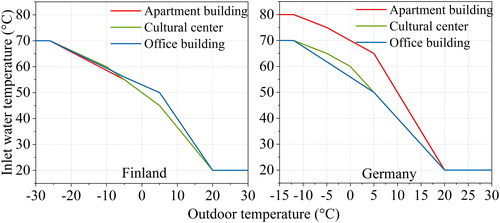
Table 6. Design powers of space heating systems.

Space heating system	Apartment building		Cultural center		Office building
	Finland	Germany	Finland	Germany	Finland	Germany
Design power at design temperature (kW)	169	225	229	175	129	101
Specific design power at design temperature (W/m^2)	35	46	58	44	54	42

Ventilation systems are depicted in Table 7. It shows the range of maximum air change rate of all rooms in one building. In the Finnish cases, design exhaust airflow rates for mechanically ventilated spaces were set according to FINVAC (2017). In the German cases, design airflow rates for mechanically ventilated spaces were selected by Seppänen et al. (2012). The air change rate of the naturally ventilated apartment building was set based on Mikola, Kalamees, and Kõiv (2017). Pressure losses of the ventilation duct system and efficiencies of fans were set according to the standard EN 13779 for all the cases (CEN 2007).

Table 7. Ventilation systems for simulated buildings.

Country	Building type	Ventilation system	Air change rate	Operation time
Finland	Apartment building	Mechanical supply and exhaust ventilation (CAV) without heat recovery	0.5 L/h	Always on
	Cultural center	Mechanical supply and exhaust ventilation (VAV with CO2 control) with heat recovery (65%) except toilets, basement, and technical spaces	0.35–5.4 L/s, m^2	8 am–10 pm
		Mechanical supply and exhaust ventilation (CAV) for basement, toilets, and technical spaces	0.35–4.5 L/s, m^2
	Office building	Mechanical supply and exhaust ventilation (VAV with CO2 control) with heat recovery (65%) for meeting rooms	0.35–3 L/s, m^2	6 am–6 pm for workdays
		Mechanical supply and exhaust ventilation (CAV) for office rooms and hallway	0.35–1.5 L/s, m^2
Germany	Apartment building	Natural ventilation	0.24 L/h	Always on
	Cultural center	Mechanical supply and exhaust ventilation (CAV) without heat recovery for kitchen, restaurant, basement, and hall	1.7–2.36 L/s, m^2	8 am–10 pm 7 am–10 pm (Basement)
		Mechanical exhaust ventilation (CAV) for toilets	2.5–4.5 L/s, m^2	Always on
		Natural ventilation for other spaces	0.2–0.43 L/s, m^2	Always on
	Office building	Mechanical supply and exhaust ventilation (CAV) without heat recovery	2.1 L/s, m^2	6 am–6 pm for workdays

Internal heat gains and domestic hot water

Internal heat gains of occupants were simulated using an activity level of 1.2 MET with a clothing of 0.75 ± 0.25 clo, which refers to sedentary activity and normal clothing (SFS-EN-ISO 7730 2006). Table 8 delineates the usage time of the buildings and annual internal heat gains of equipment and lighting, which were calculated according to these usage times and specific heat gains defined for the apartment building, the cultural center (Ministry of Environment 2017), and the office building (Martin 2017). For the German apartment building, the heating energy demand of domestic hot water (DHW) was chosen to be 17 kWh/m² (Loga and Imkeller-Benjes 1997), while it was 35 kWh/m² for the Finnish one (Ministry of Environment 2017). The heating energy demand of DHW for the cultural center and office building was assumed to be the same in both countries, at 4 and 6 kWh/m², respectively (Ministry of Environment 2017).

Table 8. Usage time and annual internal heat gains.

Parameters	Apartment building	Cultural center	Office building
Usage time	Continuous	8 am–9 pm (everyday)	8 am–4 pm (workdays)
Annual internal heat gains of lighting (kWh/m^2·a)	15.9	29.1	18.3
Annual internal heat gains of equipment (kWh/m^2·a)	11.3	14.7	3.7

Rule-based demand response control

Trend of district heat price

The moving future 24-h price of DH was known and control signals (CS) were calculated by the Behrang–Sirén method (Alimohammadisagvand, Jokisalo, and Sirén 2018; Vand et al. 2020; Ju et al. 2021). In this article, the previously mentioned rule-based demand response control (Behrang–Sirén method) was employed because of the simplicity, easy implementation, and low computational power demand. The price trend is decreasing, increasing, or flat with values −1, +1, or 0, respectively. Therefore, according to these price trend values, indoor air temperature set-points were chosen as 20 °C, 23 °C, or 21 °C. Marginal value, hourly energy (DH) price (HEP), and its future average HEP are used together to decide control values. The control signal is formed as shown here: (1) $$\begin{array}{c}If\left\{\begin{array}{c}\mathit{HEP}<HE{P}_{\mathit{avr}}^{+1,+24}-m\mathit{arginal}\hspace{0.5em}\mathit{value}\\ or\\ HE{P}_{\mathit{avr}}^{+6,+12}>HE{P}_{\mathit{avr}}^{+6,+24}+\mathit{marginal}\hspace{0.5em}\mathit{value}\end{array}\right\},\mathit{Then}\hspace{0.5em}CS=+1\\ E\mathit{lseif}\hspace{0.5em}\mathit{HEP}>HE{P}_{\mathit{avr}}^{+1,+24},\mathit{Then}\hspace{0.5em}CS=-1\\ E\mathit{lse}\hspace{0.5em}CS=0\\ End\hspace{0.5em}If\end{array}$$(1) where HEP^+1 + 24_avr is the future average HEP from hour 1 to hour 24, €/MWh; HEP^+6 + 12_avr is the future average HEP from hour 6 to hour 12, €/MWh; and HEP^+6 + 24_avr is the future average HEP from hour 6 to hour 24, €/MWh.

If the marginal value is small, the HEP will more often be smaller than the 24-hour average price minus the marginal value. Similarly, HEP^+6 + 12_avr will more often be higher than the sum of HEP^+6 + 24_avr and the marginal value. Therefore, the control signals more often have a value of +1 for charging, and the price trend is classified as increasing. A higher marginal value represents the opposite situation and raises the threshold of the further price trend, judged as increasing. For comparison, marginal values of 15 €/MWh and 75 €/MWh were applied in this study based on Martin (2017). According to the preceding analysis, the number of control signals with +1 reduces with marginal value 75 €/MWh in both the Finnish and German synthetic DH prices. In addition, since the Finnish synthetic DH price fluctuates more than the German synthetic DH price with a higher standard deviation, with the same marginal value, control signals of the Finnish synthetic DH price more often have the value +1.

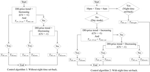
Set-point control algorithm

Two demand response control algorithms for space heating were adopted (Martin 2017): control algorithm 1 without nighttime set-back applied only for the apartment buildings, and control algorithm 2 with nighttime set-back for the cultural centers and office buildings (Figure 5). They control the hourly indoor air temperature by the space heating system. In both algorithms, T_{SH, min} is the minimum indoor temperature (20 °C), T_{SH, max} is the maximum indoor temperature (23 °C), and T_{SH, norm} is the normal indoor temperature (21 °C). To avoid overheating, a limiting outdoor temperature was chosen to be 0 °C based on Martin (2017). Differing from control algorithm 1, a nighttime set-back mode was employed in control algorithm 2, which dropped the temperature set-point T_{SH, set} to the nighttime temperature set-point T_{SH, night} (18 °C) during the unoccupied hours (10 pm–6 am).

Fig. 5. Control algorithms 1 and 2 for space heating.

Set-point smoothing

Set-point upward smoothing was applied after set-point calculation. As shown in Figure 6, this allows the set-point temperature to increase smoothly and gradually, instead of jumping from a lower temperature to higher one abruptly, thus preventing additional peaks in heating power demand.

Fig. 6. Smoothed set-points for a day of cases with nighttime set-back.

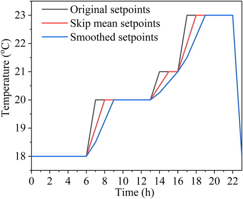
Two techniques were adopted, skip mean and hanning. First, set-points obtained based on control algorithms were calculated by skip mean as depicted in Equation 2(2) $$T_{SH,n}^{\mathit{Skip\hspace{0.5em}}\mathit{mean}}=0.5T_{SH,\mathit{Set},n-1}+0.5T_{SH,\mathit{Set},n,}\hspace{0.5em}if\hspace{0.5em}n=2,3,\dots ,N\mathit{\hspace{0.5em}and\hspace{0.5em}}{T}_{SH,\mathit{Set},n}>T_{SH,\mathit{Set},n-1}$$(2) . The skip mean technique weighed two adjacent hourly values of T_SH,set with factor 0.5. The final smoothed set-points were calculated based on these skip mean set-points by hanning technique as shown in Equation 3(3) $$T_{SH,n}^{\mathit{Smoothing}}=\{\begin{array}{c}0.5T_{SH,n-1}^{\mathit{Skip\hspace{0.5em}}\mathit{mean}}+0.5T_{SH,n}^{\mathit{Skip\hspace{0.5em}}\mathit{mean}},\hspace{0.5em}if\hspace{0.5em}n=2\mathit{\hspace{0.5em}and\hspace{0.5em}}{T}_{SH,\mathit{set},n}>T_{SH,\mathit{set},n-1}\\ 0.25T_{SH,n-2}^{\mathit{Skip\hspace{0.5em}}\mathit{mean}}+0.25T_{SH,n-1}^{\mathit{Skip\hspace{0.5em}}\mathit{mean}}+0.5T_{SH,n}^{\mathit{Skip\hspace{0.5em}}\mathit{mean}},\hspace{0.5em}if\hspace{0.5em}n=2,3,\dots ,N\mathit{\hspace{0.5em}and\hspace{0.5em}}{T}_{SH,se,n}>T_{SH,\mathit{set},n-1}\end{array}$$(3) . The hanning technique weighed three adjacent skip mean set-points with factor 0.25, 0.25, and 0.5, respectively: (2) $$T_{SH,n}^{\mathit{Skip\hspace{0.5em}}\mathit{mean}}=0.5T_{SH,\mathit{Set},n-1}+0.5T_{SH,\mathit{Set},n,}\hspace{0.5em}if\hspace{0.5em}n=2,3,\dots ,N\mathit{\hspace{0.5em}and\hspace{0.5em}}{T}_{SH,\mathit{Set},n}>T_{SH,\mathit{Set},n-1}$$(2) (3) $$T_{SH,n}^{\mathit{Smoothing}}=\{\begin{array}{c}0.5T_{SH,n-1}^{\mathit{Skip\hspace{0.5em}}\mathit{mean}}+0.5T_{SH,n}^{\mathit{Skip\hspace{0.5em}}\mathit{mean}},\hspace{0.5em}if\hspace{0.5em}n=2\mathit{\hspace{0.5em}and\hspace{0.5em}}{T}_{SH,\mathit{set},n}>T_{SH,\mathit{set},n-1}\\ 0.25T_{SH,n-2}^{\mathit{Skip\hspace{0.5em}}\mathit{mean}}+0.25T_{SH,n-1}^{\mathit{Skip\hspace{0.5em}}\mathit{mean}}+0.5T_{SH,n}^{\mathit{Skip\hspace{0.5em}}\mathit{mean}},\hspace{0.5em}if\hspace{0.5em}n=2,3,\dots ,N\mathit{\hspace{0.5em}and\hspace{0.5em}}{T}_{SH,se,n}>T_{SH,\mathit{set},n-1}\end{array}$$(3) where n is the hourly index for selected indoor air temperature set-point and N is the total number of set-points, which is 8760.

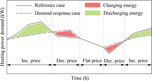
Definition of flexibility factors

Figure 7 delineates the calculation principle of flexibility factors applied in this study. The solid line is the demand curve without DR actions. The dotted line is the curve with DR actions. The red areas represent the moment when the energy price trend is increasing and the indoor temperature set-point is set to the maximum. Energy is stored mainly in building structures during the charging period. The green areas represent the opposite situation and heating power demand is lower because heat energy charged to the building structures releases with the decrease of the indoor air temperature.

Fig. 7. Charging and discharging energies during increasing and decreasing price trends.

Power flexibility factors were introduced as shown in Equations 4(4) $$P^{+}=P_{\mathit{temp},\mathit{inc}.}-P_{\mathit{ref}}$$(4) and 5(5) $$P^{-}=P_{\mathit{temp},\mathit{inc}.}-P_{\mathit{ref}}$$(5) (Stinner, Huchtemann, and Müller 2016). Heating power demand represents the total DH power of the building, which includes space heating, ventilation, and DHW: (4) $$P^{+}=P_{\mathit{temp},\mathit{inc}.}-P_{\mathit{ref}}$$(4) (5) $$P^{-}=P_{\mathit{temp},\mathit{inc}.}-P_{\mathit{ref}}$$(5) where P_ref is the power demand of reference cases without DR, kW; P_temp,inc is the power demand when the indoor air temperature increases, kW; P_temp,dec is the power demand when the indoor air temperature decreases, kW; P⁺ is the hourly power difference for charging compared with the reference case, kW; and P⁻ is the hourly power difference for discharging, kW. Since the rule-based DR control only changes the hourly space heating power, P⁺ and P⁻ represent the differences in space heating demand. Moreover, owing to the adoption of nighttime set-back, power demand increases when the indoor air temperature set-point rises after this mode. Similarly, when the indoor air temperature set-point drops down to T_SH,night, power demand decreases. Therefore, charged and discharged power caused by price changes and nighttime set-back are both considered in the calculation. Charging or discharging energy is calculated according to Equations 6(6) $$q_{\mathit{charging}}={\int }_0^{{\tau }_{\mathit{charging}}}{P}^{+}\cdot dt$$(6) and 7(7) $$q_{\mathit{discharging}}={\int }_0^{{\tau }_{\mathit{discharging}}}{P}^{-}\cdot dt$$(7) , respectively: (6) $$q_{\mathit{charging}}={\int }_0^{{\tau }_{\mathit{charging}}}{P}^{+}\cdot dt$$(6) (7) $$q_{\mathit{discharging}}={\int }_0^{{\tau }_{\mathit{discharging}}}{P}^{-}\cdot dt$$(7) where q_charging is the charged energy of a single charging period compared with a reference case without DR, kWh; q_discharging is the discharged energy of a single discharging period, kWh; τ_charging is the hours of a single charging period, h; and τ_discharging is the hours of a single discharging period, h.

The seasonal energy flexibility factors are shown in Equations 8(8) $$F{F}^{+}=\frac{{\int }_0^{{\tau }_{hs}}{p}^{+}.dt}{{\int }_0^{{\tau }_{hs}}{p}_{\mathit{ref}}.dt}$$(8) and 9(9) $$F{F}^{-}=\frac{{\int }_0^{{\tau }_{hs}}{p}^{-}.dt}{{\int }_0^{{\tau }_{hs}}{p}_{\mathit{ref}}.dt}$$(9) : (8) $$F{F}^{+}=\frac{{\int }_0^{{\tau }_{hs}}{p}^{+}.dt}{{\int }_0^{{\tau }_{hs}}{p}_{\mathit{ref}}.dt}$$(8) (9) $$F{F}^{-}=\frac{{\int }_0^{{\tau }_{hs}}{p}^{-}.dt}{{\int }_0^{{\tau }_{hs}}{p}_{\mathit{ref}}.dt}$$(9) where FF⁺ is the percentage of charged energy during the heating season compared with a reference case without DR; FF⁻ is the percentage of discharged energy; and τ_hs is the hours of the heating season, h.

Results

The simulation cases include both reference cases without DR control and DR-controlled cases. The reference cases were simulated with a constant indoor temperature set-point of 21 °C allowed to compare the DR controlled cases with variable indoor air temperature set-points. Table 9 lists the details of different simulation cases for different building types. Set-point smoothing was used for the DR cases except for the Finnish apartment building case FAB-DR-15-NS, which is a comparison to analyze the smoothing effects. Nighttime set-back was applied in the cultural center and office building DR cases. To investigate nighttime set-back effects, one case (FOB-DR-15) of the office building in Finland was simulated without nighttime set-back.

Table 9. Simulation cases for different building types.

Country	Building type	Cases	Marginal value with DR (€/MWh)	Nighttime set-back mode
Finland	Apartment building	FAB (Reference)	No DR	–
		FAB-DR-15-NS	15	–
		FAB-DR-15	15	–
		FAB-DR-75	75	–
	Cultural center	FCC(Reference)	No DR	–
		FCC-DR-15-NT	15	√
		FCC-DR-75-NT	75	√
	Office building	FOB (Reference)	No DR	–
		FOB-DR-15	15	–
		FOB-DR-15-NT	15	√
		FOB-DR-75-NT	75	√
Germany	Apartment building	GAB (Reference)	No DR	–
		GAB-DR-15	15	–
		GAB-DR-75	75	–
	Cultural center	GCC (Reference)	No DR	–
		GCC-DR-15-NT	15	√
		GCC-DR-75-NT	75	√
	Office building	GOB (Reference)	No DR	–
		GOB-DR-15-NT	15	√
		GOB-DR-75-NT	75	√

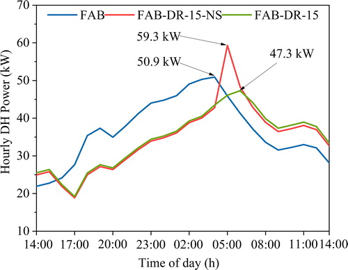
Smoothing of set-points

In order to illustrate the set-point smoothing effects, the Finnish DR-controlled apartment building without set-point smoothing (FAB-DR-15-NS) was simulated with marginal value 15 €/MWh. Figure 8 describes the hourly DH power for the 24-h example period in the reference case without DR (FAB) and the DR cases with and without smoothing (FAB-DR-15 and FAB-DR-15-NS). It indicates that the DR control without smoothing creates additional peaks in power demand. During the example period, the peak power demand of the DR control case without smoothing (FAB-DR-15-NS) is 8.4 kW higher than in the reference case without DR (FAB) and 12 kW higher than the DR control case with smoothing (FAB-DR-15). Because of this advantage, upward set-point smoothing was applied in all the cases analyzed in the following sections.

Fig. 8. The effect of DR and set-point smoothing on hourly DH power demand.

Set-point variations

Variations of indoor temperature set-points during the heating season are analyzed in this section with the Finnish and German synthetic DH prices. Figure 9 describes the range of the hours for which the algorithms set the set-point to 23 °C, 20 °C, and 18/20 °C per month during the heating season, with the Finnish synthetic DH price and marginal value 15 €/MWh. Whiskers in these box charts show the values for the minimum to maximum. The interquartile range is from 25% to 75% of these. For example, in February, the maximum number of charging hours is 48, which means that the temperature set-point was maintained continuously at 23 °C for 48 hours.

Fig. 9. Set-point variation hours in Finnish cases for each month with marginal value 15 €/MWh.

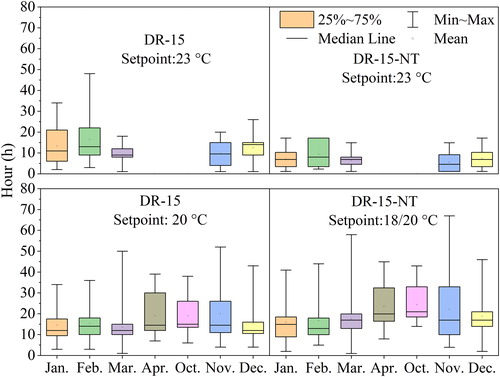
To understand the relationship between the DH price and set-point variations, the results shown in Table 1 and Figure 9 are compared. The Finnish synthetic DH price has lower average prices and standard deviations in April and October, which leads to no charging hours, for example, in the DR-15 condition. On the contrary, February has the maximum hourly price and largest standard deviation, which results in the longest charging period. Compared with the condition DR-15-NT (see Figure 9), which applied nighttime set-back, the maximum hours for charging per month decrease to close to 15, and the maximum discharging hours increase. This is mainly because the DR control was only adopted during the daytime and the indoor air temperature was maintained at 18 °C from 10 pm to 6 am.

To compare different marginal value and price effects, Table 10 shows the number of total set-point variation hours in the Finnish and German cases for each month during the heating season. For the Finnish cases, for example, with the condition DR-15, there are 201 charging hours in total when the indoor temperature was set to 23 °C in January. Contrary to the cases with marginal value 15 €/MWh, the cases with marginal value 75 €/MWh have only 5 or 3 charging hours, which can be considered almost no charging actions during the heating season. The reason is that the higher marginal value decreases the possibility that the control signal is set to +1. Moreover, the cases with marginal value 75 €/MWh have a higher number of discharging hours each month.

Table 10. Number of total set-point variation hours in Finnish and German cases for each month during the heating season.

Country	Condition	Set-point temperature (°C)	January	February	March	April	October	November	December	Total hours
Finland	DR-15	23	201	215	119	0	0	78	175	788
		20	354	247	366	419	458	401	369	2614
	DR-15-NT	23	112	123	74	0	0	34	90	433
		18/20	511	438	543	566	586	556	547	3747
	DR-75	23	0	0	0	0	0	0	5	5
		20	455	358	413	419	458	442	415	2960
	DR-75-NT	23	0	0	0	0	0	0	3	3
		18/20	583	502	574	566	586	575	563	3949
Germany	DR-15	23	1	0	0	0	0	0	5	6
		20	436	415	510	470	533	472	441	3277
	DR-15-NT	23	1	0	0	0	0	0	3	4
		18/20	478	450	556	528	569	517	489	3587
	DR-75	23	0	0	0	0	0	0	5	5
		20	436	415	510	470	533	472	441	3277
	DR-75-NT	23	0	0	0	0	0	0	3	3
		18/20	478	450	556	528	569	517	489	3587

In the German cases, there were almost no charging hours. Compared with the Finnish synthetic price, the German synthetic DH price is flatter with smaller deviations (see Tables 1 and 2). Based on Equation 1(1) $$\begin{array}{c}If\left\{\begin{array}{c}\mathit{HEP}<HE{P}_{\mathit{avr}}^{+1,+24}-m\mathit{arginal}\hspace{0.5em}\mathit{value}\\ or\\ HE{P}_{\mathit{avr}}^{+6,+12}>HE{P}_{\mathit{avr}}^{+6,+24}+\mathit{marginal}\hspace{0.5em}\mathit{value}\end{array}\right\},\mathit{Then}\hspace{0.5em}CS=+1\\ E\mathit{lseif}\hspace{0.5em}\mathit{HEP}>HE{P}_{\mathit{avr}}^{+1,+24},\mathit{Then}\hspace{0.5em}CS=-1\\ E\mathit{lse}\hspace{0.5em}CS=0\\ End\hspace{0.5em}If\end{array}$$(1) , the marginal value 75 €/MWh decreases charging hours. However, since the German synthetic DH price fluctuates relatively slightly around the average price, there are almost no charging hours with marginal value 15 €/MWh. Thus, as shown in Table 10, the change of marginal values has almost no impact on set-point variations. Moreover, in each condition, the number of discharging hours is higher than the charging hours of each month. Although the marginal value changes, charging and discharging hours in April and October are the same because of their price characteristics.

Table 11 lists the number of total set-point variation periods per month in Finnish and German cases during the heating season. In the Finnish conditions, the lower marginal value makes the control signals more sensitive to price variations. Combining the results of Tables 1, 10, and 11, condition DR-15 shows that, as the standard deviation of Finnish synthetic DH price decreases, the number of total set-point variation hours and periods also decrease each month. Although the application of nighttime set-back decreases the number of total charging hours in these Finnish conditions, the total number of periods for charging hardly changes in each month. The total number of periods for discharging increases with the increase of total discharging hours per month except in April and October.

Table 11. Number of total set-point variation periods per month in Finnish and German cases during the heating season.

Country	Condition	Set-point temperature (°C)	January	February	March	April	October	November	December
Finland	DR-15	23	15	13	13	0	0	8	14
		20	24	16	27	22	24	20	24
	DR-15-NT	23	17	15	13	0	0	7	14
		18/20	32	26	31	24	24	25	29
	DR-75	23	0	0	0	0	0	0	1
		20	21	16	23	22	24	18	24
	DR-75-NT	23	0	0	0	0	0	0	1
		18/20	26	21	27	24	24	23	27
Germany	DR-15	23	1	0	0	0	0	0	1
		20	29	35	44	45	48	25	33
	DR-15-NT	23	1	0	0	0	0	0	1
		18/20	29	34	40	44	44	28	31
	DR-75	23	0	0	0	0	0	0	1
		20	29	35	44	45	48	25	33
	DR-75-NT	23	0	0	0	0	0	0	1
		18/20	29	34	40	44	44	28	31

For the German conditions, because of the flatter price characteristic, the direct relationship between the German synthetic DH price and set-point variations is ambiguous. There are more discharging periods in March, April, and October. Although the application of nighttime set-back increases the number of total discharging hours in each month, the number of total discharging periods decreases in some months.

Impacts on charging and discharging energies

This section analyzes the charging and discharging energies of DR cases. The purpose of this summarization is to illustrate the ways in which these simulated buildings behave with the rule-based DR control from the perspective of DH producers.

Charging and discharging energies of Finnish cases

Charging and discharging energies were calculated based on Equations 6(6) $$q_{\mathit{charging}}={\int }_0^{{\tau }_{\mathit{charging}}}{P}^{+}\cdot dt$$(6) and 7(7) $$q_{\mathit{discharging}}={\int }_0^{{\tau }_{\mathit{discharging}}}{P}^{-}\cdot dt$$(7) . Figure 10 shows the variation, median, and mean values of charging and discharging energies of each charging or discharging period per month in the three building types during the heating season. For the apartment building cases, with a marginal value 15 €/MWh, the maximum charging energy during a single charging period reaches 968 kWh in February, which is close to the heat storage capacity of a fully mixed 28-m³ water tank with ΔT of 30 K. The Finnish synthetic DH price and the Helsinki outdoor temperature combined affect the charging and discharging energies. February is the coldest month with the longest charging period for 48 hours with the condition DR-15, which results in the highest maximum charging energy during the heating season. January, November, and December are colder months with higher price standard deviations, which results in relatively higher maximum charging and discharging energies. However, the mean charging and discharging energies are all close to 200 kWh except in April and October. This indicates that the maximum charging and discharging energies change with the changes of Finnish synthetic DH price standard deviation per month. With the marginal value 75 €/MWh, there are obvious decreases for charging energy maximum and mean values because of the reduction of charging hours.

Fig. 10. Variations of charging/discharging energies during a single charging/discharging period in the Finnish apartment building (FAB), cultural center (FCC), and office building (FOB) with marginal values of 15 €/MWh and 75 €/MWh.

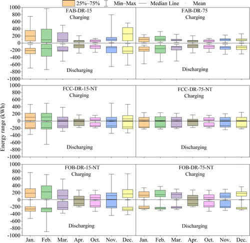
Nighttime set-back was employed in the Finnish cultural center and office building. The higher marginal value 75 €/MWh weakens the price fluctuation effects in both the Finnish cultural center and office building cases, which is consistent with the previous analysis. If nighttime set-back is applied, the maximum charging energies of January, February, November, and December are quite similar. This indicates that the application of nighttime set-back also weakens the price fluctuation impact on maximum charging and discharging energies. In accordance with the apartment building results, in the Finnish cultural center and office building February has the highest maximum discharging energy. Compared with the cultural center, the maximum and mean charging energies per month are higher in the office building. Moreover, because the same numbers of charging and discharging hours happen in April and October with different marginal values, in each type of building, the charging and discharging energies in these two months are the same.

Table 12 shows the total specific charging and discharging energies of Finnish cases per month and for the whole heating season. Months with a more fluctuating DH price and a colder outdoor temperature have a higher amount of total specific charging and discharging energies. In case FAB-DR-15, the total specific charging and discharging energies are almost balanced per month and the total specific discharging energy is 0.3 kWh/m² more than the charging energy of the whole heating season. In case FAB-DR-75, the total specific charging energy of the whole heating season reduces by nearly half compared with case FAB-DR-15. Moreover, the amount of total specific discharging energy of the heating season reduces by 30%. Charging energy decreased because of the reduction of charging hours, which resulted in less energy storage. Thus, less energy was released when the indoor air temperature dropped down, which caused less discharging energy. Similarly, in the Finnish cultural center and office building cases, when the marginal value increased, only 70–80% of the total specific energy is charged or discharged during the heating season. The total specific charging energy during the whole heating season is significantly higher in the office building compared to other building types. It is more than twice that of the cultural center with marginal value 15 €/MWh. The reason is the more intermittent use of the office building and its ventilation system (see Tables 7 and 8). There are no internal heat gains during the weekends, which affects indoor temperatures and space heating demand. In addition, the ventilation system only operated during workdays, which decreased the heat provided by the ventilation system compared with other buildings. Since the DR control only worked on space heating, space heating consumption has more obvious changes in the office building, which results in a higher amount of specific charging and discharging energies.

Table 12. Total specific charging and discharging energies of the Finnish cases per heated net floor area.

Cases	Total specific charging energy (kWh/m^2)
	January	February	March	April	October	November	December	Heating season
FAB-DR-15	1.2	1.1	0.9	0.3	0.3	0.7	1.2	5.6
FAB-DR-75	0.4	0.4	0.5	0.3	0.3	0.4	0.5	2.9
FCC-DR-15-NT	1.5	1.5	1.2	0.4	0.5	1.0	1.4	7.5
FCC-DR-75-NT	0.8	0.8	0.8	0.4	0.5	0.8	0.9	5.1
FOB-DR-15-NT	3.6	3.4	2.9	1.2	1.5	2.4	3.3	18.3
FOB-DR-75-NT	2.5	2.3	2.2	1.2	1.4	2.1	2.6	14.4
Total specific discharging energy (kWh/m^2)
FAB-DR-15	−1.1	−0.9	−1.0	−0.5	−0.5	−0.8	−1.0	−5.9
FAB-DR-75	−0.7	−0.6	−0.7	−0.5	−0.5	−0.6	−0.6	−4.2
FCC-DR-15-NT	−1.9	−1.8	−1.6	−0.8	−1.1	−1.5	−1.7	−10.3
FCC-DR-75-NT	−1.5	−1.3	−1.4	−0.8	−1.1	−1.3	−1.5	−8.8
FOB-DR-15-NT	−4.0	−3.8	−3.4	−1.6	−2.2	−3.0	−3.6	−21.7
FOB-DR-75-NT	−3.2	−2.9	−3.0	−1.6	−2.2	−2.8	−3.2	−19.0

Charging and discharging energies of German cases

Table 10 illustrates that the set-points of the German synthetic DH price with different marginal values are nearly the same. Figure 11 shows the charging and discharging energies of each period per month in the German cases. It also indicates that different marginal values have no impact on the charging and discharging energies. The maximum charging energies are quite similar from January to October in the apartment building, and are lower compared to other building types with nighttime set-back. The highest maximum charging energy appears in December in the office building. It reaches 351 kWh, which is close to the heat storage capacity of a fully mixed 10-m³ water tank with ΔT of 30 K. The change trend for mean and maximum charging energies per month ​is consistent, and both increase with the decrease of the average Hamburg outdoor temperature in the cultural center and office building cases.

Fig. 11. Variations of charging/discharging energies during a single charging/discharging period in the German apartment building (GAB), cultural center (GCC), and office building (GOB) with marginal values of 15 €/MWh and 75 €/MWh.

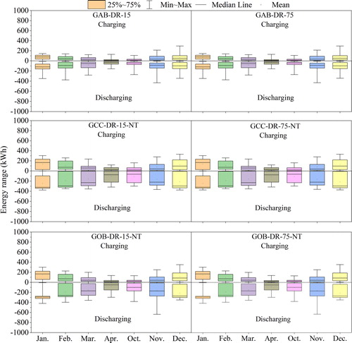
Table 13 shows the total specific charging and discharging energies of German cases per month and during the whole heating season. Similar to the Finnish cases, the amount of total specific charging and discharging energies in the office building during the whole heating season is higher compared to the other building types. The total specific charging energy of German office building during the heating season is more than three times that of the apartment building, while it is only 2.4 kWh/m² more than that of the cultural center. Compared with the Finnish apartment building and office building, less specific charging energy is needed in the German ones during the heating season. Although the Hamburg outdoor temperature is higher, the total specific charging energies per month in the German case GCC-DR-15 are quite close to those of the Finnish cultural center case FCC-DR-15.

Table 13. Total specific charging and discharging energies of the German cases per heated net floor area.

Cases	Total specific charging energy (kWh/m^2)
	January	February	March	April	October	November	December	Heating season
GAB-DR-15	0.5	0.4	0.4	0.2	0.2	0.4	0.5	2.7
GAB-DR-75	0.5	0.4	0.4	0.2	0.2	0.4	0.5	2.7
GCC-DR-15-NT	1.5	1.2	1.0	0.6	0.6	1.0	1.5	7.3
GCC-DR-75-NT	1.5	1.2	1.0	0.6	0.6	1.0	1.5	7.3
GOB-DR-15-NT	2.2	1.7	1.3	0.6	0.6	1.3	2.0	9.7
GOB-DR-75-NT	2.2	1.7	1.3	0.6	0.6	1.3	2.0	9.7
Total specific discharging energy (kWh/m^2)
GAB-DR-15	−0.9	−0.8	−0.8	−0.4	−0.6	−0.8	−0.8	−5.1
GAB-DR-75	−0.9	−0.8	−0.8	−0.4	−0.6	−0.8	−0.8	−5.1
GCC-DR-15-NT	−2.6	−2.3	−2.2	−1.5	−1.7	−2.1	−2.6	−15.0
GCC-DR-75-NT	−2.6	−2.3	−2.2	−1.5	−1.7	−2.1	−2.6	−15.0
GOB-DR-15-NT	−4.1	−3.5	−3.4	−1.8	−2.5	−3.3	−3.9	−22.5
GOB-DR-75-NT	−4.1	−3.5	−3.4	−1.8	−2.5	−3.3	−3.9	−22.5

Nighttime set-back effects on power demand

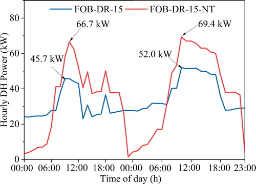
In order to analyze the nighttime set-back effects on power demand, the Finnish office building was simulated without nighttime set-back with marginal value 15 €/MWh. According to Equations 4(4) $$P^{+}=P_{\mathit{temp},\mathit{inc}.}-P_{\mathit{ref}}$$(4) and 5(5) $$P^{-}=P_{\mathit{temp},\mathit{inc}.}-P_{\mathit{ref}}$$(5) , Figure 12 depicts variations of power flexibility factors in cases FOB-DR-15 and FOB-DR-15-NT. It illustrates that P⁺ values increased significantly when nighttime set-back was adopted. The maximum P⁺ per month in cases with nighttime set-back increases at least 56% except in December. Moreover, the mean P⁺ per month has an increase of 20–80%. The reason is that when indoor temperature increases from 18 °C to 21 or 23 °C this needs more heating power than increases from 20 °C to 21 or 23 °C. Figure 13 describes the hourly DH power for two example days in January of the Finnish office building case with DR (FOB-DR-15) and with DR and nighttime set-back (FOB-DR-15-NT). It depicts that there is an obvious decrease in the DH power during the unoccupied hours (10 pm–6 am) because of nighttime set-back. However, this also causes a significant increase of the heating power in the early morning, and because of the large thermal mass of the office building, the heating power is higher throughout the day until the nighttime set-back is activated. Moreover, it indicates that when nighttime set-back is applied, additional peaks are created. The peak demand for FOB-DR-15-NT reaches 69.4 kW and the maximum difference is 21 kW, compared with the Finnish building case without nighttime set-back (FOB-DR-15), which runs counter to the DR control purpose for peak shaving.

Fig. 12. Power flexibility factors P⁺ and P⁻ of the Finnish office building without and with nighttime set-back.

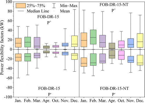
Fig. 13. Hourly heating power demand with (red line) and without (blue line) nighttime set-back in the Finnish office building.

Impacts on energy flexibility

Table 14 lists the seasonal energy flexibility factors that were calculated according to Equations 8(8) $$F{F}^{+}=\frac{{\int }_0^{{\tau }_{hs}}{p}^{+}.dt}{{\int }_0^{{\tau }_{hs}}{p}_{\mathit{ref}}.dt}$$(8) and 9(9) $$F{F}^{-}=\frac{{\int }_0^{{\tau }_{hs}}{p}^{-}.dt}{{\int }_0^{{\tau }_{hs}}{p}_{\mathit{ref}}.dt}$$(9) and average indoor temperatures of Finnish and German cases. The temperatures describe average indoor temperature conditions of the building during the entire heating season (T_ave) or during the occupied hours in the heating season (T_ave,occ). They were calculated as weighted average by the volume of the rooms. T_ave and T_{ave, occ} are the same for apartment buildings because of their continuous usage. For the cultural center and office building with nighttime set-back, T_{ave, occ} values increase about 0.4–0.7 °C compared with the T_ave values. Buildings that have higher FF⁺ values and FF⁻ lower values have lower average temperatures. However, the change of FF⁺ and FF⁻ values has almost no effect on these average temperatures during occupied hours. This illustrates that although DR control makes the building more flexible, the indoor air temperature was maintained in an acceptable range during working hours.

Table 14. Flexibility factors and average indoor temperature of Finnish and German cases.

Country	Case	FF^+ (%)	FF^− (%)	Average temperature, Tave (°C)	Average temperature during occupied hours, Tave, occ (°C)
Finland	FAB-DR-15	7.7	−8.1	21.3	21.3
	FAB-DR-75	4.0	−5.8	21.1	21.1
	FCC-DR-15-NT	8.5	−11.6	21.1	21.6
	FCC-DR-75-NT	5.7	−10.0	20.9	21.4
	FOB-DR-15	18.0	−18.9	21.4	21.5
	FOB-DR-15-NT	25.9	−30.7	20.5	21.2
	FOB-DR-75-NT	20.4	−26.9	20.3	20.9
Germany	GAB-DR-15	3.1	−6.0	21.2	21.2
	GAB-DR-75	3.1	−6.0	21.2	21.2
	GCC-DR-15-NT	6.5	−13.4	20.8	21.5
	GCC-DR-75-NT	6.5	−13.4	20.8	21.5
	GOB-DR-15-NT	8.4	−19.6	20.5	20.9
	GOB-DR-75-NT	8.4	−19.6	20.5	21.0

Absolute values of FF⁻ are always higher than FF⁺ values in all the cases, which leads to energy saving. It can also be seen from Table 14 that the Finnish cases with marginal value 15 €/MWh are more flexible than these with marginal value 75 €/MWh. However, since the German synthetic DH price is relatively flatter, energy flexibility factors are the same with different marginal values. Moreover, the Finnish office building cases FOB-DR-15 and FOB-DR-15-NT illustrate that cases with nighttime set-back have higher FF⁺ values and lower FF⁻ values, which means that more energy was charged and discharged.

Moreover, overall, FF⁺ values for the Finnish apartment and office buildings are higher than for the German ones. FF⁻ values of the Finnish apartment and office buildings are lower than for the German ones. This illustrates that the DR-controlled apartment and office buildings located in colder areas with a more fluctuating DH price are more flexible. However, although the Hamburg outdoor temperature is higher, the Finnish and German cultural center cases have similar energy flexibility values because of the higher U values of windows and the airtightness in the German cultural center. The office building cases have higher FF⁺ values and FF⁻ lower values in both Finland and Germany. A higher percentage of energy was charged and discharged during the DR control because of more intermittent usage of the office building and its ventilation system.

Discussion

In order to reduce CO₂ emissions and realize climate neutrality, a more flexible DH energy network is required to increase the proportion of renewable sources to the energy system. The advantages of DR for prosumers have been comprehensively analyzed in previous papers (De Coninck and Helsen 2016; Miller and Senadeera 2017; Zafar et al. 2018). This article investigates ways in which DR affects the power and energy flexibility of three types of district heated buildings from the perspective of DH producers. The analysis of heat stored and discharged provides references for different building type actions on DR control with different prices and weather conditions. For DH producers, this kind of analysis could be valuable for the system operation. Moreover, the maximum charging energy of each charging period for each type of building can be obtained. In a DH system, different types of buildings are connected in the same network. If TES, such as a centralized hot water storage tank, is installed in a DH system to provide storage capacity, this kind of analysis can effectively approximate water tank capacity. The results also indicate that the studied demand response control can significantly shape the heating power demand of the buildings and increase the flexibility of the energy use, which can also make the DH system flexible.

Set-point smoothing makes the indoor air temperature increase gradually, which decreases the peak power demand. The obtained results show that the DR control without smoothing creates additional peaks in power demand, while set-point smoothing significantly decreases the peak power demand compared to that case. The adoption of set-point smoothing can weaken the rebound effect, and this could be an action to consider in the DR control. In addition, although set-point smoothing was adopted, the rebound effect in these cases with nighttime set-back was still obvious. Analysis reveals that the application of nighttime set-back causes additional peaks, which is detrimental for the DH system operation. Rebound effect and additional peaks of heating power should be prevented in the selection of the control strategies. Otherwise, a significant increase of power demand can be caused in the early morning, which runs counter to the original DR intention of reducing peak energy consumption. Therefore, whether to adopt nighttime set-back during the coldest period needs to be considered, because the DH system operates at full capacity. Moreover, the asynchronization of ending times in nighttime set-back mode applied to buildings connected to the same DH network would help to minimize the peaks caused by the nighttime set-back.

Set-point variations were analyzed, and this intuitively provides the impact of energy prices on control signals. When the set-point increased to 23 °C, it resulted in charging periods. Conversely, when the set-point temperature was set to 18 or 20 °C, there were discharging periods. However, the method was different for calculating charging and discharging energies. Because of the thermal mass, there was a delay when the indoor temperature changed. Therefore, the charging energy cannot be calculated according to the charging hours counted by set-points. When the difference between DR cases and reference cases was above zero, this extra share of energy was classified as charging energy. Conversely, when the difference between DR cases and reference cases was below zero, this extra share of energy was discharging energy. During the simulation, because of set-point changes, hourly power became different from the reference cases. Some differences, relatively small and less than 1 kW, were also calculated as charging or discharging energy. This is one reason that there is charging energy for the months without charging hours. The other reason is that for the periods when indoor air temperature increased from 18 or 20 °C to normal temperature, more energy was needed. This method calculates all the energy changed share and fully considers the impact of massive building structures on power demand.

This study investigated DR actions with two country-specific dynamic prices. Results indicate that the level of fluctuation has a major role in the amount of charging and discharging energies and flexibilities in buildings. The amount of charging and discharging energies in buildings increases with a more fluctuating dynamic price and this also makes the buildings more flexible. Moreover, the choice of marginal values of the control algorithm has a key role in building energy flexibilities. Marginal values can be chosen freely. Considering the analysis of different marginal values effects (Alimohammadisagvand, Jokisalo, and Sirén 2018; Martin 2017), marginal values of 15 and 75 €/MWh were chosen because their larger difference made notable differences in the operation of the control algorithm. A lower marginal value is more sensitive and active for price changes, which leads to more charging actions. However, from the perspective of energy consumption, the more energy is stored in thermal mass, the more energy is lost. However, with higher marginal values, there are fewer charging hours and energy loss is minor. The analysis of different marginal value effects also indicated that higher ones have higher energy saving potential and more costs were saved, while the difference in cost saving rate was no more than 1% (Alimohammadisagvand, Jokisalo, and Sirén 2018; Martin 2017). However, a lower marginal value makes the DR-controlled buildings more flexible. This can better meet the purpose of increasing the proportion of renewable energy and reduce CO₂ emissions.

The results of this study are applicable to the studied building types with similar climate conditions and price characteristics of the DH energy. Once the heat generators change, the price profile will also change, which results in different control signals. However, the methodology applied in this study is general. Although the results in this study are specific for certain types of buildings, weather conditions, and prices, the rule-based DR control and simulation method could be employed in any types of buildings with different climate conditions and prices. In addition, the control algorithms only control space heating power demand. The DHW power demand impact on peak power of the building and heating system is not taken into consideration. Their cooperative actions could offer a further topic for control algorithm examination.

Conclusions

This study investigates the effect of the rule-based DR control algorithm on heating power and energy flexibility with three types of district heated buildings, the apartment building, the cultural center, and the office building, in both Finland and Germany. Two different marginal values, 15 and 75 €/MWh, were adopted in the control algorithms. In addition, two country-specific DH prices were employed: the Finnish synthetic DH price and the German synthetic DH price.

According to the results, the application of set-point smoothing weakens the rebound effect. The DH peak power demand decreases compared with the case without smoothing. The application of nighttime set-back can effectively save energy during the periods with an absence of occupants. However, it causes additional peaks, which is detrimental to the DH system operation, especially for the coldest periods.

For the hourly DH prices, the lower marginal value is more sensitive and active for price changes, which leads to more charging actions, while the higher marginal value weakened the price fluctuation effects. Compared with the Finnish synthetic DH pric used, the German synthetic DH price used was flatter with a smaller deviation, which caused marginal value changes to have no impact on set-points.

The studied demand response control can significantly shape the heating power demand of the buildings and increase the flexibility of the energy use. The range of seasonal energy flexibility factors is from 3 to 26% for charging and from −6 to −31% for discharging, depending on the building types and countries. The maximum and mean charging energies of a single charging period are mainly affected by the hourly DH price and the outdoor temperature. A more fluctuating hourly DH price and a lower outdoor temperature result in higher maximum and mean charging energies of charging periods. The indoor air temperature was also maintained in an acceptable range during working hours with DR control. Compared with the apartment building and cultural center, the office building cases have a higher percentage of charging and discharging energies because of the more intermittent usage of office building and its ventilation system.

Acknowledgments

This study is part of the Smart Proheat–Smart Prosumer Heating Technologies, SUREFIT, and FINEST Twins projects. The Smart Proheat project is funded by Business Finland and private companies Caverion Ltd., Fourdeg Ltd., Halton Ltd., and Aalto University, as well as the Federal Ministry for Economic Affairs and Energy of Germany in the project EnEff:Wärme SmartProHeaT: Smart Prosumer Heating Technologies, Subproject: Integration of Smart Prosumers Into Smart Thermal Grids (project number 03ET1598). The SUREFIT project is funded by the European Union (Horizon 2020 programme, grant number 894511). The FINEST Twins project is funded by the European Union (Horizon 2020 program, grant number 856602) and the Estonian government. For support and fruitful discussions the authors thank the steering group of the Smart Proheat project, M.Sc. Olli Nummelin and M.Sc. Nelli Melolinna from Caverion Ltd., M.Sc. Markku Makkonen from Fourdeg Ltd., and Dr. Panu Mustakallio from Halton Ltd., and colleagues from University of Applied Sciences Hamburg: M.Sc. Jan Trosdorff, M.Sc. Moritz Verbeck, and Prof. Dr. Hans Schäfers.

References

- Ala-Kotila, P., T. Vainio, and J. Heinonen. 2020. Demand response in district heating market—Results of the field tests in student apartment buildings. Smart Cities 3(2):157–71. doi:https://doi.org/10.3390/smartcities3020009
- Alimohammadisagvand, B., J. Jokisalo, and K. Sirén. 2018. Comparison of four rule-based demand response control algorithms in an electrically and heat pump-heated residential building. Applied Energy 209:167–79. doi:https://doi.org/10.1016/j.apenergy.2017.10.088
- BMU (Federal Ministry for the Environment, Nature Conservation and Nuclear Safety). 2019. Climate action in figures. Accessed September 4, 2020. https://www.bmu.de/en/topics/climate-energy/climate/climate-action-in-figures.
- Bring, A., P. Sahlin, and M. Vuolle. 1999. Models for building indoor climate and energy simulation—A report of IEA SHC Task 22: Building energy analysis tools. Stockholm, IEA. Accessed April 9, 2021. https://www.equa.se/dncenter/T22Brep.pdf.
- Bundesnetzagentur. 2014. Biogas-Monitoringbericht 2014—Bericht der Bundesnetzagentur über die Auswirkungen der Sonderregelungen für die Einspeisung von Biogas in das Erdgasnetz [Biogas Monitoring Report 2014—Report of the German Bundesnetzagentur on the effects of the special regulations for the feed-in of biogas into the natural gas grid]. Post und Eisenbahnen. Bonn. Accessed November 10, 2020. https://www.bundesnetzagentur.de/SharedDocs/Downloads/DE/Sachgebiete/Energie/Unternehmen_Institutionen/ErneuerbareEnergien/Biogas/Biogas_Monitoring/Biogas_Monitoringbericht_2014.pdf?__blob=publicationFile&v=1.
- Cai, J., and J. E. Braun. 2019. Assessments of demand response potential in small commercial buildings across the United States. Science and Technology for the Built Environment 25 (10):1437–55. doi:https://doi.org/10.1080/23744731.2019.1629245
- CEN (The European Committee for Standardization). 2007. EN. 2007. 13779: 2007. Ventilation for non-residential buildings–performance requirements for ventilation and room-conditioning systems. Brussels, Belgium: The European Committee for Standardization.
- De Coninck, R., and L. Helsen. 2016. Quantification of flexibility in buildings by cost curves–Methodology and application. Applied Energy 162:653–65. doi:https://doi.org/10.1016/j.apenergy.2015.10.114
- DWD, Deutscher Wetterdienst (German Meteorological Service). 2017. Handbuch Ortsgenaue Testreferenzjahre von Deutschland für mittlere, extreme und zukünftige Witterungsverhältnisse (Handbook of Precise Test Reference Years of Germany for Medium, Extreme and Future Weather Conditions). Accessed September 11, 2020. https://www.bbsr.bund.de/BBSR/DE/forschung/programme/zb/Auftragsforschung/5EnergieKlimaBauen/2013/testreferenzjahre/try-handbuch.pdf?__blob=publicationFile&v=3.
- DWD. 2020. Wetter und Klima aus einer Hand [Weather and climate from a single source]. Accessed September 11, 2020. https://kunden.dwd.de/obt.
- EN 15251. 2007. Indoor environmental input parameters for design and assessment of energy performance of buildings addressing indoor air quality, thermal environment, lighting and acoustics. Finnish Standards Association SFS, Helsinki.
- Equa Simulation, A. B. 2010a. Validation of IDA indoor climate and energy 4.0 with respect to CEN Standards EN 15255-2007 and EN 15265-2007. Solna, Sweden. Accessed April 9, 2021. http://www.equaonline.com/iceuser/validation/CEN_VALIDATION_EN_15255_AND_15265.pdf.
- Equa Simulation, A. B. 2010b. Validation of IDA indoor climate and energy 4.0 build 4 with respect to ANSI/ASHRAE Standard 140-2004. EQAU Simulation Technology Group, Sweden. Accessed April 9, 2021. http://www.equaonline.com/iceuser/validation/ASHRAE140-2004.pdf.
- Euroheat & Power, & Moczko, D. 2019. District energy in Germany. Accessed April 4, 2021. https://www.euroheat.org/knowledge-hub/district-energy-germany.
- European Commission. 2018. EU Climate Action—2030 climate and energy framework. Accessed September 4, 2021. https://ec.europa.eu/clima/policies/strategies/2030_en.
- European Commission. 2020. 2050 long-term strategy. Accessed September 24, 2020. https://ec.europa.eu/clima/policies/strategies/2050_en.
- Finnish Government. 2019. Programme of Prime Minister Sanna Marin’s Government 10 December 2019. Inclusive and competent Finland—A socially, economically and ecologically sustainable society. Accessed September 4, 2020. http://urn.fi/URN:ISBN:978-952-287-811-3.
- Finnish Society of Indoor Air Quality (Sisäilmayhdistys ry). 2018. Sisäilmastoluokitus 2018 [Classification of indoor environment 2018]. Helsinki: Finnish Society of Indoor Air Quality.
- FINVAC (The Finnish Association of HVAC Societies). 2017. Opas ilmanvaihdon mitoitukseen muissa kuin asuinrakennuksissa [The guidelines of ventilation dimensioning in other buildings than apartment building]. FINVAC. Helsinki. Accessed April 9, 2021. https://finvac.org/wp-content/uploads/2020/06/Opas_ilmanvaihdon_mitoitukseen_muissa_kuin_asuinrakennuksissa_2017.pdf.
- FMI (Finnish Meteorological Institute). 2020. Energialaskennan testivuodet nykyilmastossa [Test years for energy calculation in current climate]. Accessed September 11, 2020. http://ilmatieteenlaitos.fi/energialaskennan-testivuodet-nyky.
- Gelazanskas, L., and K. A. Gamage. 2014. Demand side management in smart grid: A review and proposals for future direction. Sustainable Cities and Society 11:22–30. doi:https://doi.org/10.1016/j.scs.2013.11.001
- Hedegaard, R. E., M. H. Kristensen, T. H. Pedersen, A. Brun, and S. Petersen. 2019. Bottom-up modelling methodology for urban-scale analysis of residential space heating demand response. Applied Energy 242:181–204. doi:https://doi.org/10.1016/j.apenergy.2019.03.063
- IEA (International Energy Agency). 2018. Energy policies of IEA countries: Finland 2018 review, IEA, Paris. Accessed September 4, 2020. https://www.iea.org/reports/energy-policies-of-iea-countries-finland-2018-review.
- Jensen, S. Ø., A. Marszal-Pomianowska, R. Lollini, W. Pasut, A. Knotzer, P. Engelmann, A. Stafford, and G. Reynders. 2017. IEA EBC annex 67 energy flexible buildings. Energy and Buildings 155:25–34. doi:https://doi.org/10.1016/j.enbuild.2017.08.044
- Johra, H., P. Heiselberg, and J. Le Dréau. 2019. Influence of envelope, structural thermal mass and indoor content on the building heating energy flexibility. Energy and Buildings 183:325–39. doi:https://doi.org/10.1016/j.enbuild.2018.11.012
- Ju, Y., J. Jokisalo, R. Kosonen, V. Kauppi, and P. Janßen. 2021. Analyzing energy flexibility by demand response in a Finnish district heated apartment building. In E3S Web of Conferences (Vol. 246, p. 09006). EDP Sciences. doi:https://doi.org/10.1051/e3sconf/202124609006
- Junker, R. G., A. G. Azar, R. A. Lopes, K. B. Lindberg, G. Reynders, R. Relan, and H. Madsen. 2018. Characterizing the energy flexibility of buildings and districts. Applied Energy 225:175–82. doi:https://doi.org/10.1016/j.apenergy.2018.05.037
- Kalamees, T., K. Jylhä, H. Tietäväinen, J. Jokisalo, S. Ilomets, R. Hyvönen, and S. Saku. 2012. Development of weighting factors for climate variables for selecting the energy reference year according to the EN ISO 15927-4 standard. Energy and Buildings 47:53–60. doi:https://doi.org/10.1016/j.enbuild.2011.11.031
- Kontu, K., J. Vimpari, P. Penttinen, and S. Junnila. 2018. City scale demand side management in three different-sized district heating systems. Energies 11 (12):3370. doi:https://doi.org/10.3390/en11123370
- Le Dréau, J., and P. Heiselberg. 2016. Energy flexibility of residential buildings using short term heat storage in the thermal mass. Energy 111:991–1002. doi:https://doi.org/10.1016/j.energy.2016.05.076
- Loga, T., and U. Imkeller-Benjes. 1997. Energiepass Heizung/Warmwasser [Energy demand heating/hot water]. Institut Wohnen und Umwelt (IWU). Darmstadt. Accessed April 9, 2021. https://www.iwu.de/fileadmin/tools/ephw/1997_IWU_LogaImkeller-Benjes_Energiepass-Heizung-Warmwasser-EPHW.pdf.
- Martin, K. 2017. Demand response of heating and ventilation within educational office buildings. Master’s thesis, Aalto University.
- Mikola, A., T. Kalamees, and T. A. Kõiv. 2017. Performance of ventilation in Estonian apartment buildings. Energy Procedia 132:963–8. doi:https://doi.org/10.1016/j.egypro.2017.09.681
- Miller, W., and M. Senadeera. 2017. Social transition from energy consumers to prosumers: Rethinking the purpose and functionality of eco-feedback technologies. Sustainable Cities and Society 35:615–25. doi:https://doi.org/10.1016/j.scs.2017.09.009
- Ministry of Environment. 2017. Ympäristöministeriön asetus uuden rakennuksen energiatehokkuudesta [Decree 1010/2017 Ministry of Environment’s decree on new building’s energy efficiency]. Ministry of Environment. Helsinki. Finland. Accessed April 9, 2021. https://www.finlex.fi/fi/laki/alkup/2017/20171010#Pidp4469784.80.
- Moosberger, S. 2007. IDA ICE CIBSE-validation: Test of IDA indoor climate and energy version 4.0 according to CIBSE TM33, issue 3. EQAU Simulation Technology Group, Sweden. Accessed April 9, 2021. http://www.equaonline.com/iceuser/validation/ICE-Validation-CIBSE_TM33.pdf.
- Nuytten, T., B. Claessens, K. Paredis, J. Van Bael, and D. Six. 2013. Flexibility of a combined heat and power system with thermal energy storage for district heating. Applied Energy 104:583–91. doi:https://doi.org/10.1016/j.apenergy.2012.11.029
- Oldewurtel, F., D. Sturzenegger, G. Andersson, M. Morari, and R. S. Smith. 2013. Towards a standardized building assessment for demand response. In 52nd IEEE Conference on Decision and Control, pp. 7083–7088.
- Palensky, P., and D. Dietrich. 2011. Demand side management: Demand response, intelligent energy systems, and smart loads. IEEE Transactions on Industrial Informatics 7 (3):381–8. doi:https://doi.org/10.1109/TII.2011.2158841
- Reynders, G., J. Diriken, and D. Saelens. 2017. Generic characterization method for energy flexibility: Applied to structural thermal storage in residential buildings. Applied Energy 198:192–202. doi:https://doi.org/10.1016/j.apenergy.2017.04.061
- Reynders, G., R. A. Lopes, A. Marszal-Pomianowska, D. Aelenei, J. Martins, and D. Saelens. 2018. Energy flexible buildings: An evaluation of definitions and quantification methodologies applied to thermal storage. Energy and Buildings 166:372–90. doi:https://doi.org/10.1016/j.enbuild.2018.02.040
- Robert, F. C., G. S. Sisodia, and S. Gopalan. 2018. A critical review on the utilization of storage and demand response for the implementation of renewable energy microgrids. Sustainable Cities and Society 40:735–45. doi:https://doi.org/10.1016/j.scs.2018.04.008
- Sahlin, P. 1996. Modelling and simulation methods for modular continuous systems in buildings. Stockholm, Sweden: Royal Institute of Technology.
- Salo, S., A. Hast, J. Jokisalo, R. Kosonen, S. Syri, J. Hirvonen, and K. Martin. 2019. The impact of optimal demand response control and thermal energy storage on a district heating system. Energies 12 (9):1678. doi:https://doi.org/10.3390/en12091678
- Sandrock, M., C. Maaß, S. Weisleder, C. Kaufmann, G. Fuß, P. A. Sørensen, L. L. Jensen, and K. Radmann. 2016. Erneuerbare Energien im Fernwärmenetz Hamburg – Teil 1: Handlungsoptionen für einen kurzfristigen Ersatz des Kraftwerks Wedel [Renewable Energies for district heating in Hamburg – Part 1: Options for action for a short-term replacement of the Wedel combined heat and power plant]. HIC Hamburg Institut Consulting GmbH. Hamburg. Accessed November 10, 2020. https://www.hamburg-institut.com/images/pdf/studien/161207%20%20Bericht%20BUE.pdf.
- Seppänen, O., N. Brelih, G. Goeders, and A. Litiu. 2012. Health based ventilation guidelines for Europe. Work package 5. Existing buildings, building codes, ventilation standards and ventilation in Europe. The Final Report. REHVA. Brussels. Accessed April 9, 2021. https://webgate.ec.europa.eu/chafea_pdb/assets/files/pdb/20091208/20091208_d05_oth5_en_ps.pdf.
- SFS-EN-ISO 7730. 2006. Ergonomics of the thermal environment. Analytical determination and interpretation of thermal comfort using calculation of the PMV and PPD indices and local thermal comfort criteria. Helsinki: Finnish Standards Association.
- Shan, K., S. Wang, C. Yan, and F. Xiao. 2016. Building demand response and control methods for smart grids: A review. Science and Technology for the Built Environment 22 (6):692–704. doi:https://doi.org/10.1080/23744731.2016.1192878
- Suhonen, J., J. Jokisalo, R. Kosonen, V. Kauppi, Y. Ju, and P. Janßen. 2020. Demand response control of space heating in three different building types in Finland and Germany. Energies 13 (23):6296. doi:https://doi.org/10.3390/en13236296
- Stinner, S., K. Huchtemann, and D. Müller. 2016. Quantifying the operational flexibility of building energy systems with thermal energy storages. Applied Energy 181:140–54. doi:https://doi.org/10.1016/j.apenergy.2016.08.055
- Vand, B., K. Martin, J. Jokisalo, R. Kosonen, and A. Hast. 2020. Demand response potential of district heating and ventilation in an educational office building. Science and Technology for the Built Environment 26 (3):304–19. doi:https://doi.org/10.1080/23744731.2019.1693207
- Yoon, J. H., Baldick, R., & Novoselac, A. 2016. Demand response control of residential HVAC loads based on dynamic electricity prices and economic analysis. Science and Technology for the Built Environment 22 (6):705–719.
- Zafar, R., Mahmood, A., Razzaq, S., Ali, W., Naeem, U., & Shehzad, K. 2018. Prosumer based energy management and sharing in smart grid. Renewable and Sustainable Energy Reviews 82:1675–1684.