Coalition for Disaster Resilient Infrastructure (CDRI) 2022 Conference Proceedings

2

Exploring action agenda and adaptive pathways for disaster resilient infrastructure: the outcome of the DRI Technical Conference 2022CONTACT Ratnesh Kumar [email protected]

ABSTRACT

The Coalition for Disaster Resilient Infrastructure (CDRI) aims to enhance global understanding and action on climate and disaster resilient infrastructure (DRI) through knowledge creation, curation and dissemination. In this direction, CDRI organized its first DRI Technical Conference on 12–13 October 2022 in New Delhi, India. The Conference was complemented by a Special Issue of the journal Sustainable and Resilient Infrastructure (Taylor & Francis), officially launched at COP 27 in Sharm el-Sheikh, Egypt. The two complimenting initiatives – the Conference and the special issue – are targeted to create lasting contributions towards mainstreaming the DRI agenda. The Conference and Special Issue publication both focused on ‘Adaptive Pathways for Disaster Resilience’ as an approach for resilience-building before, during and after disaster events, from a systems perspective. The papers presented at the Conference provided rich evidence and insights on the current state of play on Adaptive Pathways for Resilient Infrastructure. The Conference provided a range of actions to be explored by CDRI with its member countries, organizations, the private sector and other partners to support resilience.

KEYWORDS:

• Action agenda
• adaptive pathways
• CDRI
• disaster resilient infrastructure (DRI)
• DRI technical conference

Funding

This work was supported by the Coalition for Disaster Resilient Infrastructure (CDRI).

1. Introduction

The Coalition for Disaster Resilient Infrastructure (CDRI) aims to enhance global understanding and action on climate and disaster resilient infrastructure (DRI) through knowledge creation, curation and dissemination. In this direction, CDRI organized its first DRI Technical Conference on 12–13 October 2022 in New Delhi, India. The Conference was complemented by a Special Issue of the journal Sustainable and Resilient Infrastructure (Taylor & Francis), officially launched at COP 27 in Sharm el-Sheikh, Egypt. The two complimenting initiatives – the Conference and the Special Issue – are targeted to create a lasting contribution towards mainstreaming the DRI agenda.

1.1. Theme

The Conference and Special Issue publication both focused on ‘Adaptive Pathways for Disaster Resilience’ as an approach for resilience-building before, during and after disaster events, from a systems perspective. Infrastructure development is typically undertaken for a 10- to 50-year horizon. However, current challenges of unprecedented disasters, impacts of climate change, and rapid evolution of problems and their solutions necessitate frequent but incremental improvements in the infrastructure systems. This helps infrastructure systems face current disasters with better preparedness and greater resilience against future hazards.

Systemic interconnections within and among infrastructure systems also induce new complexities and vulnerabilities for infrastructure. Adaptive pathways can provide a deeper understanding of infrastructure systems in diverse scenarios to inform future development through incremental but progressive planning and action over time.

In essence, the adaptive pathways approach can help stakeholders in dealing with immediate challenges without compromising current benefits and deliver long-term development dividends.

Despite the vast potential of adaptive pathways as a concept, it’s actionable understanding requires collation of relevant knowledge and experiences. The first iterations of the DRI Technical Conference and Special Issue were focused on addressing these gaps along the following subthemes:

(1) Dynamic disaster and climate change risk assessments for resilient infrastructure development.

(2) Strengthening stakeholder participation and collaboration for adaptive pathways towards resilient infrastructure.

(3) Implementation of adaptive pathways to foster resilience in complex and interdependent infrastructure systems across sectors.

1.2. Approach

The Conference was designed in two parts. The first part featured interactive presentations of 25 high-quality research papers selected through an open call. All the sessions were curated for informed and thought-provoking discussions by over 70 practitioners and researchers with diverse backgrounds from 16 countries.

In the second part, a closing ceremony of the Conference was held at New Delhi on 13 October 2022 with a wider audience to commemorate the International Day for Disaster Reduction.

2. Overview of adaptive pathways

The papers presented at the Conference provided rich evidence and insights into the current state of play on ‘Adaptive Pathways for Resilient Infrastructure’. An adaptive pathways approach begins by integrating system designs with flexible processes for continued improvement without affecting the system’s overall performance in the long term (Sánchez-Silva & Acuña-Coll, 2022). Performances of critical infrastructure systems are subject to impacts of climate change and disasters which require their systemic assessments. Deeper implications of such vulnerabilities, potential solutions and benefits of resilience were vividly revealed in the case studies conducted at the University of Oxford on the transportation networks of four African countries (Pant, Jaramillo & Hall, 2022). Efforts to build resilience across infrastructure systems necessitate managing diverse stakeholders within and across sectors to align their competing objectives, and require partnerships at all levels (Keam & Harrington, 2022). Efforts towards resilience need frameworks and decision support tools for conscious performance assessment with a feedback loop for policymakers, industry and community (Ziv et al., 2022). Further, efforts and investment in resilient infrastructure can be made financially more attractive by expanding the valuation paradigm of net present worth to include disaster risks, related losses and benefits to stakeholders (Espinoza, 2022).

Several key issues, implications and potential solutions for proposing adaptive pathways for resilient infrastructure were presented at the Conference. Some of the salient issues are listed here:

• Digital tools integrated with hazard and climate modelling, as well as asset vulnerability assessment, can play a vital role in formulating adaptive solutions to go beyond risk assessment and build resilience (Boothroyd, Williams & Hoey, 2022; Dahal & Gnyawali, 2022; Dalal et al., 2022; Gupta & Nikam, 2022; Kamepalli, 2022; Kloss & Samimi, 2022; Nakum et al., 2022; Sánchez-Silva & Acuña-Coll, 2022; 129). For example, InfraRiveChange – a web-based GIS application developed by CDRI fellows, can map river migration and risks to bridges (Boothroyd, Williams & Hoey, 2022).

• Vulnerability assessment and retrofitting of existing infrastructure can improve resilience with marginal time and cost (Banerjee & Matsagar, 2022; Dalal et al., 2022; Joo & Sinha, 2022; Parol & Al-Sanad, 2022). Several technologically viable solutions are emerging, such as base isolations of existing hospital buildings for resilience to earthquakes developed by a CDRI fellow (Banerjee & Matsagar, 2022).

• Adaptive planning requires specific capacity among the stakeholders, and availability and demand for such capability needs to be mapped and augmented (Estrain & Srinivasan, 2022).

• A higher education curriculum related to disaster management and infrastructure resilience needs to be developed considering the mainstreaming of technical innovations, interdisciplinarity, industry practices and policy planning (Johnson & Bajaz, 2022).

• Some models are available to quantify the losses from disasters, but there is a need to develop frameworks and models for economic analysis of investing in resilience and avoided losses from disasters (Narendr, Aithal & Das, 2022; Pal et al., 2022; Vithean et al., 2022).

• Adaptive disaster mitigation measures can have several additional non-tangible benefits. For example, urban open spaces can help as a tool to reduce urban heat and flood, but these can also improve the quality of air and lifestyles (Nivya, Karmakar & Sajan, 2022; Palmate & Kumar, 2022).

• Adaptive planning for inclusive resilience needs to design systems especially considering the most vulnerable members, like people with limited ability, vulnerable age groups and others (Bhangdia & Murhekar, 2022).

3. Exploring the action agenda for resilient infrastructure

Adaptive pathways require collaborative efforts by stakeholders at various levels for the creation of knowledge and informing practice. The half day workshop at the DRI Technical Conference 2022 gave a platform to delegates for exploring three streams of action agendas: Research; Advocacy; and Policy & Practice. The exercise produced several insights, ideas and opportunities as summarized in Table 1.

Table 1. Recommendations from delegates: priority actions to support adaptive pathways for DRI.

Priority Actions for Research	Priority Actions for Advocacy	Priority Actions for Policy & Practice
Develop common vocabulary to ensure consistent understanding of DRI among all stakeholders. Promote translational research on systemic risk and impact assessment considering compounding, cascading and concurrent hazards. Risk assessment and resilience modelling should include scenarios and anticipated events to accommodate increasing frequency of unprecedented events. Emphasis on social infrastructure, community problems and needs. Develop tools for quantitative post-disaster need assessment of infrastructure systems and their cascading impacts on other services. Develop scientific evidence on the potential of indigenous and traditional knowledge, skills and wisdom for resilience-building. Develop and nurture innovative solutions for critical problems on disaster resilience. Tools and solutions to include high granularity, resolution, accuracy and downscale measures for actionable and timely interventions. Promote open access research and data-sharing through suitable platforms and tools. Encourage participatory bottom-up and field-based research that is inclusive of different user groups (e.g., children as users of resilient schools). Encourage active collaborations between industry, academics and policymakers, within and across countries. Research lifecycle should be sensitive to disaster cycles and seasonality to maximize post-disaster demands. Research findings should be expressed in simple, understandable and actionable forms.	Compile relatable examples and case studies on the benefits of resilience, additional costs if any and benefits to resilient communities. Develop actionable roadmaps beyond risk assessment, e.g., adoption of codes, resilience-based design and incentives. Encourage and collate examples of legal compliance of policies on disaster management and resilience to use them as evidence for advocacy. Communicate with diverse audiences at all levels using visual tools, in local languages and dialects, through workshops, webinars, websites, video clips, fun activities and so on. Use diverse channels and platforms for advocacy using local and national media (print, digital and others). Use tailor-made communication for public, private, community and other stakeholders considering their roles, leadership and celebrity status. Encourage hackathons, advertisements, exhibitions at educational institutes, training centres and workplaces. Encourage community-led demand for resilience. Focused advocacy among investors with evidence of how resilience investment decisions augment investment benefits and add value. Promote events like the DRI Technical Conference that facilitate exchange of knowledge and experience, and develop collective thinking about resilience.	Mandate and adopt scenario- and evidence-based research approaches to inform policymaking responsive to local needs Promote adoption of local knowledge, expertise and good practices. This should cover customization of new technology and breakthrough innovations. Mainstream emerging technologies and innovations for DRI through policy and practice. Formulate resilience-based design process for infrastructure planning. Map learning needs and develop an actionable strategy for building capacity of policymakers and practitioners for mainstreaming resilience in infrastructure development interventions. Ensure community engagement in policy formulation and implementation. Promote interdepartmental collaborations among government and industry, e.g., collaborations between departments of the environment, disaster management and urban affairs for systemic urban resilience). Encourage active collaborations between industry, academics and policymakers, within and across countries. Disaster management plans, standard operating procedures and guidelines should be easily understandable by users and facilitate actionable decision-making. Conduct periodic monitoring and evaluation of policy interventions policies through on-ground feedback loops. Document the lessons gained during policy implementation through learning labs and pilot projects. Promote need-based resource allocation considering future risks and affordability. Identify and formulate policy to incentivise relevant stakeholders for adopting resilience-based design into practice.

4. 10-point action agenda for CDRI

In an increasingly interconnected and inter-dependent world, building climate and disaster resilient infrastructure (DRI) will require concerted actions by various stakeholders at all levels across the globe. The Conference provided a range of actions to be explored by CDRI with its member countries, organizations, the private sector and other partners to support the resilience of infrastructure as follows:

(1) Common vocabulary: At present DRI is perceived differently by various stakeholders. CDRI should collate and propose a common vocabulary to ensure systematic, comprehensive and consistent understanding of resilience to promote effective communication and coordination.

(2) Open and collective knowledge: Building DRI for present and future requires access and adoption of the best knowledge and practice. Efforts on resilience will greatly benefit from an open sharing of knowledge, research, databases, models, expertise and technology. CDRI should take steps to facilitate an open and collective knowledge exchange through latest technologies.

(3) Resilience in education and professional training: Unprecedented challenges posed by climate change and disasters require capacity-building and specialized professionals. There is an urgent need to develop and promote curricula on DRI at all levels, across disciplines and specializations.

(4) Systemic approach: Increasing complexity and interdependency of infrastructure assets emphasize the importance of collective resilience. CDRI should promote research, knowledge-sharing and adoption of frameworks and tools that support a systemic approach for resilience within and across infrastructure systems.

(5) Interdisciplinarity: Present capacity and research on DRI are primarily available in specific disciplines. Significant gaps exist at the interface of disciplines. There is a need to adopt an interdisciplinary approach for optimum action on resilience. CDRI can anchor a network of research centres and industry to amplify interdisciplinary capacity and knowledge.

(6)Translational research and innovation: Significant gaps exist between knowledge and their adoption in practices. CDRI should promote an innovation ecosystem to convert research findings into actionable innovations. The innovation ecosystem will encompass translational research grounded in community problems, codification of knowledge for action, technology transfer and align the research life cycle with the hazard cycle.

(7) Inclusive: COVID-19 has demonstrated that no one is safe until everybody is safe. CDRI should strive for the inclusion of specific concerns of people and communities rooted in their gender, age, physical ability, income, geography and across all its initiatives.

(8) Demonstrate and document benefits of resilience: Experiences around the world show that the past is no longer a good guide for future hazards, as climate uncertainty has exacerbated disaster events both in frequency and magnitude. To broad base stakeholder interest and investment in resilience, the benefits of adopting resilience must be advocated through evidence and scenario-based assessments. CDRI should promote appropriate methodologies, assessment models, and case studies of successes as well as infrastructure failures, and good practices to promote a resilience mindset.

(9)Adaptive planning: Infrastructure requires long term investments and planning. Although not all infrastructure decisions can be made now, they can be planned, prioritized and prepared to deliver a better outcome for the current and future needs of communities. Adaptative pathways are the way forward for managing uncertainty in infrastructure planning and should be adopted into governance. CDRI should continue to invest in promoting flexibility and adaptiveness in infrastructure planning such as the Special Issue of the Journal and Conference to mobilize different stakeholders on this approach.

(10) Continued engagement with research, policy and practice: The DRI Technical Conference brought together researchers, practitioners and policymakers on a common platform to exchange knowledge, share experiences and widen their understanding and partnerships for the cause of resilience. CDRI should continue to create such opportunities for collaboration among different stakeholders for promoting infrastructure resilience.

Acknowledgments

The DRI Technical Conference 2022 on Adaptive Pathways for Resilient Infrastructure is CDRI’s first research conclave, and would not have been possible without the support of our member countries, organizations and partners. We are sincerely grateful to the members of the project Appraisal and Steering Committee (ASC) – Marjorie Greene (USA), Ila Patnaik (India), Satoru Nishikawa (Japan) and Ravi Sinha (India) – for their guidance and scientific inputs on the Conference design, procurement, theme selection and facilitating discussions during the event. We are thankful to Jim W. Hall (UK) for gracing the event with a remarkable keynote address drawing from decades of research on climate change and disasters. We are also indebted to esteemed experts Patrick Lambe (Singapore, Ireland) and Ilan Noy (New Zealand) for curating the Conference sessions and creating an environment for rich discussions during the event. We are thankful to all the delegates whose hard work and high-quality research made this Conference a milestone for Adaptive Pathways for Resilient Infrastructure. We also recognize the selfless contributions of the peer reviewers in the selection of the finest research works.

We express our wholehearted gratitude to Kamal Kishore (Co-Chair, CDRI Executive Committee; & Secretary, National Disaster Management Authority, Government of India) for seeding the concept of an international conference focused on research in climate and disaster resilience infrastructure. Throughout the process, we have received strong commitment and encouragement from the leadership at CDRI, initially by Sandeep Poundrik and subsequently by Amit Prothi (Director General, CDRI). Organizing an international conference, particularly under the limitations imposed by COVID-19, required proactive support from various ministries under the government of India. We are especially grateful to Ministry of External Affairs, government of India, for crucial help in facilitating visas for international delegates.

We were fortunate to have a capable support from our event and publication partners, Informa Markets and Taylor & Francis Group. Finally, it is our pleasure to acknowledge the Conference Team and CDRI family for unwavering support during the entire Conference process.

Disclosure statement

The DRI Technical Conference 2022 was sponsored by CDRI, along with editorial work of the Conference Proceedings. However, CDRI did not influence the research, data, findings, and views presented in the research papers.

Flexible and adaptable strategies for developing sustainable and resilient infrastructureCONTACT Mauricio Sánchez-Silva [email protected] Acuña-Coll [email protected]

ABSTRACT

Recent developments in the safeguarding systems, sustainable and green taxonomies and the Intergovernmental Panel on Climate Change (IPCC) Climate Resilience Framework (amongst others) have created new processes and criteria for delivering better climate and disaster resilience for infrastructure projects and assets. There is not yet a standard risk classification methodology for climate change risk assessment or the inclusion of disaster risk within it, or within other international standards such as TCFD, ISO 14091, 92. Applying a more dynamic selection of risk receptors, risk and hazard component variables, system/asset boundaries, timeframes and socio-economic surroundings along with the exclusion of compound risk factors can improve the extent to which a disaster and climate risk assessment can deliver stronger system wide resilience and shape adaptation pathways. This paper outlines key risk assessment elements and considerations that can improve their application, using practical examples from infrastructure projects and providing specific references to assist in replication. Key elements are: (i) the inclusion of social and environmental risk receptors alongside asset/infrastructure; (ii) bringing risk classification in line with IPCC risk definitions and associated vulnerability definitions; (iii) risk analysis that informs the creation of corresponding climate and disaster management plans, systems and processes; and (iv) moving beyond a compliance mindset to use a more dynamic risk assessment to deliver positive resilience outcomes in our assets and infrastructure.

KEYWORDS:

• Climate resilience
• disaster resilience
• systems approach
• safeguarding systems
• climate risk classification

1. Introduction

The World Bank estimates that disasters cost the global economy US$520 billion annually and force 26 million people into poverty. Since the Sendai Framework for Disaster Risk Reduction (2015–2030) was adopted, some 60 million people in over 100 countries have been displaced by disaster events, mainly floods, storms and droughts (Mizutori, 2018). Although the field of disaster management has attracted significant attention, efforts toward improving long-term aspects like mitigation and recovery have been revolving around the same ideas and strategies with relatively limited advances. Governments and institutions worldwide linked with this problem need to explore new approaches in relationship with infrastructure, which is key to socioeconomic development. In this paper, we propose to rethink the problem based on a combination of two fundamental lines of thought: systems thinking and flexibility. Formulating the problem in this framework is an alternative to an increasingly bureaucratized system of emergency management in many countries, where there is pressure to do things according to some standard operating procedures. In that environment, freelancing, improvising or going outside the chain of command are discouraged. It is argued that systems thinking and flexibility are necessary to enhance the preparation and response to disasters, thus making communities more resilient, which in turn impacts their long-term welfare.

2. Pillars to enhance the response to disasters

2.1. Overview of systems thinking

During the last decades, systems thinking has emerged as a way of understanding the dynamics and complexities of the interactions among a system’s components. This not only includes physical elements, but also the system’s ‘soft’ side, such as the behaviour and response of all actors, operational decisions and the interactions among stakeholders. System thinking helps understand how subsystems and individual components interact at different levels, paying special attention to emergent properties, which leads to the widely known concept of the holistic view of projects. Systems thinking is not simply an engineering approach; rather it is a philosophy for solving many practical problems (Blockley & Godfrey, 2017). Systems thinking is supported by three main ideas: (i) structuring information hierarchically (i.e. in layers); (ii) identifying and recognizing the importance of loops; and (iii) understanding the system as a collection of processes.

The third pillar is important in understanding the system’s dynamics. Then, every system can be described as a hierarchical arrangement of processes, where every process consists of smaller internal processes. Note that the idea of process is linked with the concept of life cycle in the sense that it describes all activities or changes in the system during a given timeframe. Therefore, life cycle analysis is a way to approach engineering projects from a systems thinking perspective.

Embedded in the idea of process are the concepts of elasticity and change that are reflected in continuous adjustments directed towards maintaining functionality. Understanding infrastructure as a process provides a more dependable insight into its performance and the way it should be designed and managed through time.

2.2. Flexibility and adaptability

Flexibility is ‘the ability of a system to respond or change some of its design or operational parameters easily to keep or add value to the system when subjected to either internal or external demands’ (Sánchez-Silva & Calderón-Guevara, 2022). This definition has three fundamental elements: (i) the ability to respond/change; (ii) how this change occurs (i.e. easiness); and (iii) the purpose of change – that is, keeping or adding value to the system. In the development of engineering systems, flexibility contributes to three fundamental issues. First, it makes better use of financial resources. Secondly, by changing the design and management paradigms it contributes significantly to reducing CO² emissions and, therefore, climate change effects. Thirdly, it is the best tool for managing uncertainty, which is essential to reducing risks and increasing resilience. Flexibility is an attribute of a process; in that sense, implementing flexibility requires describing the problem from the perspective of systems thinking.

Flexible systems are equipped with specific features that facilitate future changes such as expansions or contractions of the system capacity. Incorporating flexibility within the design and operation of infrastructure and in responding to disasters is a key source of individual, organizational and societal resilience, which contributes to making better decisions and building more sustainable systems. The operation of systems that are not designed to be flexible frequently becomes expensive and inefficient since they may incur additional investments derived, for example, from over-estimating future demands.

It is important to notice that the terms flexibility and adaptability are sometimes used interchangeably. A system is said to be adaptable if it can modify its structure or functionality when required, e.g., respond to perturbations to maintain its functionality over time. Overall, flexibility is a necessary feature of adaptable systems. Introducing flexibility and adaptability as system properties is a new concept that contributes to better management of planned/unplanned events, taking advantage of investment/business opportunities, reducing possible cost overruns, and handling the perceptions and interests of stakeholders (Sánchez-Silva, 2019).

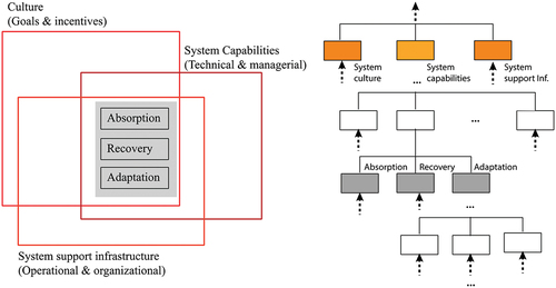
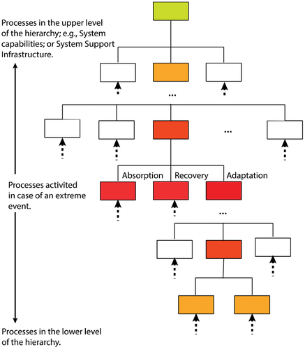
3. Underlying structure of resilient infrastructure

Based on systems thinking theory, the first task to model resilient infrastructure is to structure it as a hierarchy of processes (Figure 1). In this case, two processes are of particular interest: (i) the processes that characterize infrastructure management; and (ii) the processes needed for infrastructure response to damaging events. These two processes have elements in common and define the overall system behaviour. The former has three principal enabling elements (subsystems): culture (goals and incentives); capabilities (technical and managerial); and infrastructure (operational and organizational; Scott, 2007). These elements support and define the infrastructure’s ability to function as required and to respond to extreme events. At a lower level, there are those processes involved in the infrastructure’s response to unwanted events (e.g., resilience) (see, Figure 2); these are: (i) absorption; (ii) recovery; and (iii) adaptation (Rehak et al., 2019). Absorption describes the system’s capacity to accommodate the demand (e.g., extreme event). Recovery is the technical and managerial process by which the damaged system is put back into service. Finally, adaptation defines its capacity to adjust to a new reality.

Figure 1. Hierarchical processes that describe infrastructure resilience.

4. Systems and flexibility within the context of resilience

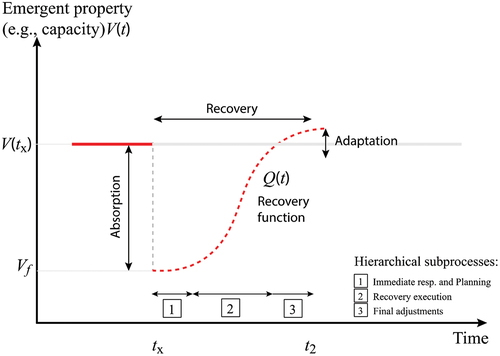
The response to events as they materialize over time, the processes shown in Figure 1, which interact continuously, need to be flexible. In other words, they cannot be planned and designed as rigid structures (protocols) that remain invariant over time. However, not all processes that describe a system carry the same level of flexibility. In a hierarchical process structure, processes in the upper levels of the hierarchical structure (e.g., system support infrastructure) occur slowly over time in comparison with those in the lower levels. For example, in the case of infrastructure, changes in upper levels require planning and the investment of a large amount of resources. On the contrary, processes in the lower levels (e.g., recovery) imply sudden or frequent changes in the system (or subsystems). In summary, the concept of flexibility has different scopes depending upon where the system assessment is made.

When modelling resilience, the focus is on those processes that are required for the system to ‘bounce back’ to its original condition as shown in Figure 2 (e.g., absorption, recovery and adaptation). This requires equipping the system with (i) the properties needed to respond to extreme events, mostly from a physical perspective; (ii) to have the infrastructure and the appropriate strategies to restate its condition as quickly as possible; and (iii) to make modifications to the system to adjust to a new reality. The concept of flexibility applied to resilient systems should be framed at least within the context defined by these processes. However, special features could be considered and studied depending upon the problem at hand. For example, in Figure 2 three additional sub-processes of the recovery are included: immediate response and planning; recovery execution; and final adjustments.

Figure 2. Description of the main processes related to resilience.

5. Definition and modelling of flexible actions

The flexibility of the system’s constitutive processes implies the possibility of an adjustment of its structure or change as required to meet some external or internal requirements. Changes can be described by actions that (i) modify its operation; (ii) its physical structure; or (iii) both. The first case is associated with changes in the way the system is managed. The second corresponds to a physical intervention that increases capacity and the corresponding operation level instantly. The third case is a physical intervention that provides a new maximum capacity (physically), but not all capacity is used at once. In this case, capacity is progressively added by means of operational decisions until the maximum defined by the new physical state is reached.

The actions mentioned above vary depending upon the level in the hierarchy of process where the decision is made. Then, in the upper parts of the hierarchy the frequency of interventions is smaller and their extension (size) larger. The ideas behind adaptation pathways (Haasnoot et al., 2013) are defined mostly at this level. Adaptation pathways emerged as a strategy to integrate a sequence of possible actions, which can be implemented progressively, depending on the system’s evolution (dynamics) over time. This approach can be used to navigate a decision tree as the future of the project unfolds; the project evolution then becomes a route through the decision tree. An Adaptation Pathways map is drawn based mostly on expert judgment and is a way to incorporate flexibility within infrastructure planning. An alternative approach has been proposed by Sánchez-Silva and Calderón-Guevara (2022) and Torres-Rincón, Bastidas-Arteaga and Sánchez-Silva (2021) in which the system state adapts continuously to accommodate changes in the demand or requirements imposed by stakeholders or external agents. In this approach, the system incorporates flexibility in the design that facilitates the system’s response.

6. Activating flexibility to make systems more resilient

Changes in the upper levels of the hierarchy are defined by decisions whose primary objective is to avoid failure and maximize the return in pursuit of the fulfilment of the system’s purpose (Figure 3). In the lower hierarchical levels, changes are related to specific tasks, for example, decisions regarding the implementation of the system’s reconstruction strategy after a disaster. These actions are dominated by concepts such as agility, efficiency and timeliness. In the case of an extreme event, a disruption occurs causing some damage and loss of functionality, which is often related to how the processes in the upper levels are handled. Immediately after the damaging event, processes in lower levels activate (e.g., recovery and adaptation). Flexibility at this level should be looked at from a different perspective than in the upper levels. It focuses on facilitating changes in the recovery process to make it more efficient.

Figure 3. Relevance of processes in the response to an extreme event.

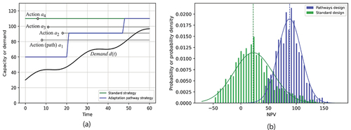
7. Illustrative examples of the value of a flexible approach

Consider the case of a system that is already in operation, which is subjected to extreme events and to an increasing demand (e.g., traffic), both of which might cause failure. For this system, a set of four feasible system interventions (actions) have been identified to enhance its capacity–adaptation pathways (Figure 4a). A model has been built to generate a large set of future random demand scenarios to evaluate the long-term response of the system in terms of its life cycle cost – i.e., expected discounted net present value (NPV). In this example, a standard (inflexible) design is compared with a flexible system. In the flexible management policy, when the system performance reaches a safety criterion, a decision is made as to what is the best action to implement – a pathway to follow; there are no predefined long-term strategies. The decision on the best pathway is made based on a 10-year prediction of the demand according to historical records. A sample path (realization) of the system performance in both cases is shown in Figure 4a, while the comparison of the expected NPV distribution (after 2000 demand scenarios) is shown in Figure 4b. The results show that flexible systems (adaptation pathways approach) are far more cost-efficient for managing systems than traditional rigid approaches, not only in terms of the mean NPV, but also when comparing the variance.

Figure 4. (a) Realization of the system response; (b) comparison of expected NPV between traditional and adaptation pathway simulation designs.

The system’s performance shown in Figure 4 is highly controlled by the processes in the upper levels of the hierarchy, i.e., processes related to the selection of adaptation paths and the definition of criteria for interventions. In case of failure, processes related to recovery become highly relevant. In this example, we focus only on the processes of absorption and recovery (Figure 2 and Figure 3). The absorption process defines the extent of damage and depends on the intensity of the extreme event and the system state (decision made at the upper level in the hierarchy). The recovery is modelled as a sigmoid function Q(t) = b/(1+ exp(-at)), with b the size of recovery in terms of the system’s capacity and a, is a constant that determines the easiness of the recovery process. Note that a is a key property of flexibility that captures the logistics and organization measures that facilitates the recovery.

Figure 5. (a) Realizations of the system response to an extreme event; (b) comparison of expected system recovery time.

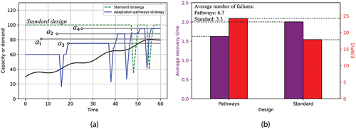
Figure 5a shows a system with a different set of potential pathways and a sample path of failure and recovery processes, both for the flexible and the standard case. Failures are defined by the rate of extreme events and the capacity and demand at a point in time. It can be noticed that decisions in strategic processes (upper levels) have an impact on resilience, mostly because they control the number and size of failures. The system was subjected to 2000 simulations of demand. Although the number of failures during the lifetime is, on average, larger for flexible systems (6.7), they have smaller recovery times (left axis in Figure 5b). In addition, the expected NPV (right axis in Figure 5b) is significantly higher when flexibility is incorporated. In summary, these results show that flexible systems are more resilient in the long term since they have smaller recovery times and larger expected NPV than standard designs.

8. Conclusions

The main conclusions of this paper can be summarized as follows:

• Modelling the performance of infrastructure in the light of disaster management and resilience should be framed within the context of systems thinking and flexibility. Systems thinking is a framework that contributes to looking at the problem of disaster management as interacting processes organized hierarchically. Flexibility is key to managing uncertainty, facilitates the unavoidable need to deal with unexpected circumstances and favours financial responsibility and sustainability.

• The concept of process is central to understanding the value of flexibility since it captures the dynamic nature of the evolution of systems over time. Flexibility facilitates changes in the route of a process or in its final objective. Incorporating flexibility in disaster management requires focusing on the process of recovery and not only on the final product.

• Incorporating flexibility in infrastructure management enhance resilience and leads to better long-term system performance. It has an advantage over traditional designs in terms of recovery times (resilience) and cost-efficiency evaluated as the expected NPV.

Disclosure statement

The DRI Technical Conference 2022 was sponsored by CDRI, along with editorial work of the Conference Proceedings. However, CDRI did not influence the research, data, findings, and views presented in the research papers.

Systemic assessment of climate risks and adaptation options for transport networks in East AfricaCONTACT Raghav Pant [email protected]

ABSTRACT

Transportation networks are lifeline systems fundamental to economic and social prosperity. Disruptions to these networks can be detrimental to long-term growth plans. This is particularly important in the context of growing climate hazards such as flooding, where long-term sustainable development, social wellbeing and economic stability are at risk from widespread failures of transport networks. In view of these threats, there is a need to create evidence of the impacts of current and future climatic risks to transport networks. To address this problem, the authors have developed and implemented a multi-regional transport infrastructure climate risk and adaptation assessment framework. This framework seeks to understand the extent and location of extreme hazard exposures, direct damage and economic flow losses, risks and adaption investment needs for strategic transport networks. It aims to inform decision-makers to help: (i) improve network resilience by identifying and strengthening the locations of highest vulnerabilities; and (ii) understand the benefits of investing in climate resilience in terms of avoided losses from climate risks. The authors apply their climate risk and adaptation assessment tool for the case study region covering Kenya, Tanzania, Uganda and Zambia, where they investigate the risks due to river and coastal flooding over current and future climate change driven scenarios. Their analysis shows that there are large benefits to investing in climate adaptation of major roads and rail network links in those countries that are exposed to flooding in the present and future. They estimate that investing in climate adaptation from the present (2019) until 2080 to strengthen resilience of the 20 most flood risk incurring roads and railways lines in the region would amount to about US$9 million and US$92 million in adaption investments, but would avoid risks as high as US$875 million and US$234 million across future climate scenarios.

KEYWORDS:

• climate risks and hazards
• resilience assessment
• climate adaptation
• economic risks
• economic risks

1. Introduction

Transport networks of roads and railways are lifelines that provide mobility and access to sustain delivery of essential commodities around the world (Hallegatte, Rentschler & Rozenberg, 2019). Such large-scale networks face risks from natural hazards, which are predicted to intensify in the future under adverse climate change (Wang et al., 2017). This will have an impact on planned transport investments, predicted to take place at record high levels of US$40 trillion or 1.8% of global gross domestic product (GDP) from 2016–2040 (Global Infrastructure Hub, 2017).

The case study countries for this paper – Kenya, Tanzania, Uganda and Zambia – are witnessing significant large-scale infrastructure investments, driven by the prospects of strong economic growth and prospects of enabling these countries to be gateways to growing domestic markets in Africa (Horvat et al., 2021). But there is a danger that climate change driven natural hazards such as flooding might be detrimental to their growth and development plans. Estimates suggest that most of Kenya experienced flooding in 2020 (Makena et al., 2021), that in Tanzania the climate hazards costs in recent years have amounted to about 1% of national GDP (Erman et al., 2019), and that in Uganda rising water levels in Lake Victoria displaced thousands of people, flooding homes and businesses, damaging infrastructure and destroying roads (Brown, 2020). Evidence also suggests that repair and recovery of damaged transport assets in these countries is either very slow or does not take place over many years. In Kenya, a survey of infrastructure flood damage in 27 out of 47 counties showed that transport assets took much longer to repair than other infrastructure (electricity and piped water); only about 6% of damaged roads and bridges were repaired within one month and 57% were never repaired (Njogu, 2021). As climate change increases the magnitudes and frequencies of catastrophic natural hazard events, incidents of transport failures resulting in socio-economic losses are likely to become more common (Schaller et al., 2016).

There is a need to create evidence of the impacts of current and future climatic hazards on transport networks. Presently, the identification of systemic risks to transport networks remain poorly understood. Responding and adapting to the threat of climate change requires a research approach that: (i) maps out where climate hazards are greatest; (ii) identifies the transport network locations exposed and vulnerable to climate hazards; (iii) assesses direct physical damage costs and indirect economic flow losses to quantify climate risks; (iv) assesses the costs and benefits (in terms of risk reduction) of adaptation options under different future development, growth and climate scenarios; and (v) prioritizes adaptation options, so that limited budgets can be used to climate-proof networks as efficiently as possible.

This paper presents research that addresses the above issues, and in doing so delivers analysis on quantifying systemic risks due to failures of key locations in the transport networks of low-income countries (LIC). We present a detailed methodology supported by novel analysis of climate change driven flooding risks and adaptation assessment of transport networks in Kenya, Tanzania, Uganda and Zambia. This research has been undertaken in the High-Volume Transport (HVT) project, ‘Decision Support Systems for Resilient Strategic Transport Networks in Low Income Countries’ (Hickford et al., 2023), which aims to support investment decisions and option selection for long-distance strategic land transport networks exposed to climate risks by creating the first multi-state transport infrastructure decision support system in a LIC context.

In the next sections we describe the methodology, case study country data and implementation, the main results and the conclusions from our study.

2. Methodology

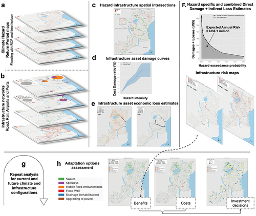
To quantify climate change driven flooding risks to transport networks on the large scale, we have developed a system-of-systems framework for transport risk and adaptation analysis. Figure 1 provides a graphical overview of this system-of-systems framework implemented for our case-study countries, which is consistent with spatial systems modelling approaches previously applied to Tanzania (Pant et al., 2018a), Vietnam (Oh et al., 2019) Argentina (Kesete et al., 2021) and the United Kingdom (Pant et al., 2018b). Briefly, the framework components (described as steps A–H) are discussed below.

2.1. Hazard assembly

We assemble flood hazard maps of various flood severities across climate scenarios and futures to initiate failure in transport systems (see, Table 2).

Table 1. Summary of relevant data sources and details. More information is provided in Hickford et al. (2023).

Category	Data	Source	Details
Hazards	River flooding	Aqueduct flood product datasets (World Resources Institute, 2020)	Flood depths in metres over grid squares (~900 m^2 at the Equator) 1/2, 1/5, 1/10, 1/25, 1/50, 1/100, 1/250, 1/500 and 1/1000 (1/return period) 5 Future climate models RCP 4.5 & 8.5 emission scenarios Epoch: Baseline (2019) + 2030, 2050 and 2080 For coastal only: With and without subsidence 5th, 50th and 95th percentile sea level rise scenario confidence
	Coastal flooding
Transport networks	Roads	OpenStreetMap (OSM)	179,000 km of motorways and trunk roads, primary roads, secondary roads and tertiary roads Assigned or assumed road properties (road pavement type, construction material, width, lanes)
	Rails	OpenStreetMap (OSM)	423 key stations, stops and halts and 10,500 km of lines identified as: currently open; under rehabilitation; construction; proposed for the future
	Ports	Various statistics from the port authorities of Kenya and Tanzania	Two main maritime ports: Kenya’s Port of Mombasa and Tanzania’s port of Dar es Salaam, with two more maritime ports in Tanzania 15 inland ports on Lake Victoria and Lake Tanganyika
	Airports	Country specific reports for aviation authorities in Kenya, Uganda, Tanzania and Zambia	Six of the largest airports with known freight carrying capacity identified in Kenya (3), Uganda (1), Tanzania (1), Zambia (1)
Direct damages	Fragility curves	Direct damage (fragility) curves for paved roads, unpaved roads and railway lines (Koks et al., 2019)	Percentage of damage an asset vs flood depth We assume that damages happen only when flood depth > 50 cm
	Rehabilitation costs	Database of 172 projects (AfDB [African Development Bank], 2014) The World Bank’s Road Costs Knowledge System (ROCKS) database (World Bank, 2018)	Generalized estimated of rehabilitation costs in US$/km for different types of paved and unpaved roads and railway lines All costs converted to 2019 US$ values
Network flows	Global import–export trade flows between countries	UN Conference on Trade and Development (UNCTAD) and World Bank (unctadSTAT website)	Flows in tons/day and US$/day mapped to specific ports, airports, road and rail border crossings in four countries Flows allocated along roads and rail lines connected to ports and airports, to locations of economic activity and population concentration Assumed 4% annual growth in freight until 2080, with future rail lines also used

Table 2. Description of adaptation options considered with costs, relevant asset types and impacts on damage curves and return period cut-offs.

Option	Description	Initial Investment Cost	Assets	Damage Curve Modification f(x) = ax + b		High Return Period Cut-offs (years)
				a	b
Swales	Detention swales, also referred to as ‘bioswales’, are broad shallow channels topped with vegetation. They are designed to attenuate and infiltrate run-off volume from adjacent impervious surfaces.	13,430 US$/km	Roads, railways	0.965	0.00	10
Spillways	To discharge flows that cannot either be used immediately or stored in a reservoir for future use.	176,193 US$/km	Roads, railways	0.900	0.00	10
Mobile flood embankments	Inflatable tube (hose) segments that are used to insulate/dam flood water.	573,068 US$/km	Roads, railways	1.000	−0.20	0
Flood wall	Freestanding, permanent, engineered structure designed to prevent encroachment of floodwaters.	1,230,000 US$/km	Roads, railways	1.000	0.00	50
Drainage rehabilitation	Dredging by removal of accumulated material from watercourses, canals or drainage systems.	46,843 US$/km	Roads paved only	0.780	−0.10	50
Upgrading to paved road	Upgrading to more climate-resilient paved roads.	247,159 US$/ lane-km	Roadsunpaved only	Assign paved damage curve		0

2.2. Multi-modal transport network assembly

We create a transport system-of-systems model by: collecting geospatial data and creating connected network models from such data; identifying network locations with attributes (e.g., road pavement type, type of rail station and so on); identifying locations for freight transport (e.g., key ports, rail stations, road connections to ports and rail); collecting freight trade data in tons/day (or US$/day) in our study region and integrating it with network locations; assigning freight flows in tons/day (or US$/day) on the specific network locations based on a least generalized cost criteria to create flow estimates. Details of these models are provided in Pant et al. (2018a) and Hickford et al. (2023).

2.3. Exposure analysis

We overlay each hazard map with each network location and estimate flood depth and lengths of each asset (road or rail link) inundated. This tells us how many roads and rail lines potentially face flood risks across all flood return periods, climate scenarios and time epochs.

2.4. Direct damage estimation

We estimate direct damage costs by: selecting a flood depth that might cause physical damage to assets; looking up vulnerability curves, which quantify the percentage (or fraction) of length of damage sustained by an asset for a given flood depth (Koks et al., 2019); and multiplying the rehabilitation costs in US$/km of each asset by its flood damage length.

2.5. Indirect economic loss estimation

For damaged assets we estimate indirect economic losses from import–export trade flow disruptions in US$/day by: finding all existing freight trade routes (mapped in Step B) which are disrupted; finding rerouting options and redirecting flows towards alternative routes to estimate losses as the increase in transport costs; and estimating flow disruptions in terms of freight tonnage lost when there are no rerouting options.

2.6. Direct and indirect risk metrics

In this study we estimate two risk metrics: expected annual damage (EAD) and expected annual economic loss (EAEL), which are respectively the measures of average damage cost (US$) and average economic loss (in US$/day) incurred for an asset in any given year due to a given hazard type for a given time epoch and climate scenario. EAD (or EAEL) is estimated as the area under the direct damage (or economic loss) versus the exceedance probability curve (1/return period; Koks et al., 2019). From the estimate of EAD and EAEL we get the asset level total risk = EAD + (duration of disruption) × EAEL/day.

2.7. Multiple failure and scenario estimations

We implement steps A–F for future climate hazard and transport scenarios.

2.8. Adaptation options assessment

After spatial risk assessment across climate scenarios and time epochs, we conduct an adaptation assessment for a set of adaptation options for building resilience to flood shocks. The effectiveness of any adaptation option is evaluated and compared through a cost–benefit analysis (CBA), where the present value (PV) of investments into an adaptation option are compared with the PV of benefits due to avoided risks over an implementation timeline of several years (Pearce, Atkinson & Mourato, 2006). The CBA analysis helps identify priority assets and locations where benefit–cost ratio $\left(\mathrm{B}\mathrm{C}\mathrm{R}=\hspace{0.17em}\frac{\mathrm{P}\mathrm{V}\mathrm{o}\mathrm{f}\mathrm{b}\mathrm{e}\mathrm{n}\mathrm{e}\mathrm{f}\mathrm{i}\mathrm{t}\mathrm{s}}{\mathrm{P}\mathrm{V}\mathrm{o}\mathrm{f}\mathrm{a}\mathrm{d}\mathrm{a}\mathrm{p}\mathrm{t}\mathrm{a}\mathrm{t}\mathrm{i}\mathrm{o}\mathrm{n}\mathrm{i}\mathrm{n}\mathrm{v}\mathrm{e}\mathrm{s}\mathrm{t}\mathrm{m}\mathrm{e}\mathrm{n}\mathrm{t}}\right)$≥1 or only target the few assets with the highest BCR. We can use this analysis to estimate the total budget needed for investing in climate adaptation for assets with BCR≥1. The next section describes the specific types of adaptation options for flooding considered in this study.

Figure 1. Graphical representation of transport system-of-systems risk and adaptation assessment framework.

3. Case study data assembly and implementation

We implement the methodological framework, through open datasets of hazards, infrastructure networks, rehabilitation costs and trade flows, which is summarized in Table 1. Here we provide some main data highlights, while all data are described in detail in Hickford et al. (2023).

Important observations from Table 1 are that we have: (i) used several flood maps capturing current and future climate change scenarios at a reasonably high spatial resolution; (ii) derived network data from open-source OSM in which the road and rail network location information is very accurate when compared to satellite imagery; (iii) considered and spatially mapped future new rail lines which are being developed in the region; (iv) included all major ports and airports that are used for large-scale freight transport in the region; (v) derived damage costs estimated from known rehabilitation project costs in the region; and (vi) mapped trade flows from a well-documented database and also built scenarios of future trade growth based on regional forecasts.

Table 2 describes the details of adaptation options and their costs derived from different sources (Hickford et al., 2023). The effectiveness of adaptation options in reducing risks are measured in terms of how they reduce the flood vulnerability of assets (damage curves) and how they provide protection up to a given return period. From Table 2 the f(x) = ax + b values show how the damage curves are linearly scaled down by each option and the right-most column shows the return periods until which the flood has no effect.

4. Results

We present selective results of the adaptation assessment for roads and railway lines in our case study region. Here we evaluate the effectiveness of the adaptation options in respect of the maximum benefits they provide. At each asset level we assume that the duration of disruptions is 15 days, which means the total risk = EAD + 15 × EAEL/day. We estimate these risks at the baseline year 2019 and the three future years 2030, 2050, 2080 under climate scenarios, and linearly interpolate risks between these years. We assume that a climate adaptation option is planned in 2019 and has a timeline of investment until 2080. We perform the CBA analysis for each option selected for each asset type that is at risk, with the adaptation options’ initial investment in 2019 and maintenance costs assumed to be 20% of initial investment costs every five years and 1% every year until 2080, with a 10% discounting rate (Hickford et al., 2023).

For a given asset we find that there could be multiple options that provide a BCR ≥ 1 estimate, which means for all these options the PV of benefits (avoided risks) outweigh the PV of adaptation investments. However, if we were to select one preferred option, then we look at the one with the highest avoided risks because it would be the most effective in reducing risks while providing a BCR ≥ 1. We apply this principle to all our assets and their adaptation options to find the most risk reducing option for assets with BCR ≥ 1, whereas for assets with BCR < 1 we select the highest BCR options.

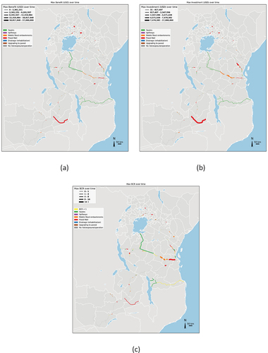
The results of our analysis with the best options for road assets with their (a) PV of benefits, (b) PV of adaptation investments and (c) BCR estimates are shown in Figure 2. These results show at several locations options such as drainage rehabilitation are most effective, while installing flood walls and swales are also effective options in many cases. We have also highlighted the assets for which BCR < 1, which shows that none of our chosen options might be useful for such assets. From these results we estimate that investing in adaptation of the top 20 most benefit incurring road investments would amount to about US$9 million in PV of adaption investments against of PV of benefits of about US$875 million in avoided risks.

Results from Figure 2 for railways show that options such as swales, flood walls and mobile flood embankments are the most effective adaptation options. We suggest that several of these options should be applied to new railway lines such as the new SGR line along the Central Corridor in Tanzania where swales could help avoid potential risks. For rail assets ranking the top 20 most benefit incurring rail investments would amount to about US$92 million PV in adaptation investments and provide US$234 million in PV of benefits (avoided risks).

Figure 2. Results of maximum (a) PV of benefits PVs; (b) PV of adaptation investments; and (c) BCR for adaptation options for roads at risk due to river and coastal flooding under climate change.

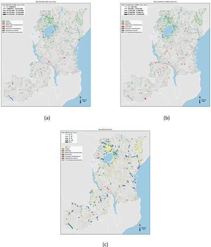
The adaptation analysis shows that most of the highest benefits and BCR > 1 ranked assets are key linkages that facilitate trade flows across whole networks at present or in the future. Such assets represent very compelling cases for investing in climate adaptation to improve systemic resilience of transport networks. With BCR results we can prioritize the assets and locations for building climate resilience, while estimating the scales of adaptation investment requirements. Results of maximum (a) PV of benefits PVs; (b) PV of adaptation investments; and (c) BCR for adaptation options for roads at risk due to river and coastal flooding under climate change.

Figure 3. Results of maximum (a) PV of benefits; (b) PV of adaptation investments; and (c) BCR for adaptation options for railways.

5. Conclusion

This paper presents findings from a comprehensive assessment of systemic risks to transport networks due to current and future climate change driven river and coastal flooding hazards. It provides an understanding of magnitudes and locations of extreme hazard exposures, damages, economic losses and risks to strategic road and railway network links, which helps make the case for: (i) improving network resilience by identifying and strengthening the locations of highest vulnerabilities; and (ii) understanding the benefits of investing in climate resilience in terms of avoided physical damages and economic losses from climate risks.

Through the demonstration of a detailed transport network climate risk and adaptation assessment, this study has satisfied its main objective of providing an analytical methodology and tool for prioritizing adaptation decision-making. The quantified direct and indirect risks, adaptation benefits and costs here will help transport planners and stakeholders in Kenya, Tanzania, Uganda and Zambia to understand the scales of climate risks they might face and how they could prioritize adaptation investments along with long-term planning objectives. The methods and tools from this study can be utilized for several other climate hazards and contexts for systemic risk assessment of transport networks on the national and regional scales.

Acknowledgments

This research was funded by UKAID through the UK Foreign, Commonwealth & Development Office under the High-Volume Transport Applied Research Programme, managed by DT Global. The authors wish to gratefully acknowledge the support and funding of FCDO for this project (HVT043). The views expressed in this report do not necessarily reflect the UK government’s official policies.

Disclosure statement

The DRI Technical Conference 2022 was sponsored by CDRI, along with editorial work of the Conference Proceedings. However, CDRI did not influence the research, data, findings, and views presented in the research papers.

Improving resilience outcomes for infrastructure: how to maximize the benefits from disaster and climate risk assessmentCONTACT Liesl Keam [email protected]

ABSTRACT

Recent developments in the safeguarding systems, sustainable and green taxonomies and the Intergovernmental Panel on Climate Change (IPCC) Climate Resilience Framework (amongst others) have created new processes and criteria for delivering better climate and disaster resilience for infrastructure projects and assets. There is not yet a standard risk classification methodology for climate change risk assessment or the inclusion of disaster risk within it, or within other international standards such as TCFD, ISO 14091, 92. Applying a more dynamic selection of risk receptors, risk and hazard component variables, system/asset boundaries, timeframes and socio-economic surroundings along with the exclusion of compound risk factors can improve the extent to which a disaster and climate risk assessment can deliver stronger system wide resilience and shape adaptation pathways. This paper outlines key risk assessment elements and considerations that can improve their application, using practical examples from infrastructure projects and providing specific references to assist in replication. Key elements are: (i) the inclusion of social and environmental risk receptors alongside asset/infrastructure; (ii) bringing risk classification in line with IPCC risk definitions and associated vulnerability definitions; (iii) risk analysis that informs the creation of corresponding climate and disaster management plans, systems and processes; and (iv) moving beyond a compliance mindset to use a more dynamic risk assessment to deliver positive resilience outcomes in our assets and infrastructure.

KEYWORDS:

• Climate resilience
• disaster resilience
• systems approach
• safeguarding systems
• climate risk classification

1. Partnerships for infrastructure

Partnerships for Infrastructure (P4I) is an Australian Government initiative partnering with Southeast Asia to drive sustainable, inclusive and resilient growth through quality infrastructure. P4I partners with Cambodia, Indonesia, Laos, Malaysia, The Philippines, Thailand, Timor-Leste, Vietnam and the Association of Southeast Asian Nations (ASEAN). P4I works with partners to strengthen infrastructure decision-making and practice across the transport, energy, utilities and telecommunications sectors. P4I provides flexible services as part of the infrastructure lifecycle, including planning and prioritization, financing strategy and procurement. P4I also advises on the overarching infrastructure policy context and sector-specific regulatory issues. The three main services offered to partners are infrastructure advisory services, linkages with Australian government agencies and other institutions, and knowledge sharing and learning. As the foundation of quality infrastructure, P4I also integrates gender equality, disability and social inclusion, as well as disaster risk reduction and climate change into its activities.

2. Developments in climate and disaster risk assessment systems

P4I is aware that recent developments in the safeguarding systems, sustainable and green taxonomies and Intergovernmental Panel on Climate Change (IPCC) Climate Resilience Frameworks (amongst others) have created new processes and criteria for delivering improved climate and disaster resilience for infrastructure projects and assets. These new developments are helping to shape P4I’s evolving approach to supporting resilient and sustainable infrastructure development.

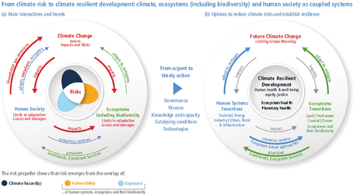
The latest updates to the Equator Principles (2020) brought them in line with the objectives of the Paris Agreement by requiring safeguards systems to include climate change risk assessment (CCRA), identifying physical risks and transition risks. However, financial institutions are delivering this requirement to varying degrees and with an assortment of methodologies. There is currently no standard risk classification methodology for this CCRA or the inclusion of disaster risk within it, or within other international standards (i.e., ISO 14091, 92, 31,000 and others). Varying selections of risk receptors, risk and hazard component variables, system/asset boundaries, timeframes and socio-economic surroundings along with the exclusion of compound risk factors mean that the extent to which a disaster and climate risk assessment can deliver system-wide resilience for the asset is often left to chance. Typically delivered from within the safeguarding systems, assessments do not reflect the growing global recognition of moving beyond ‘do no harm’ to an approach that instead delivers positive outcomes. The rapid acceleration of sustainable and green taxonomy frameworks in the wake of (and heavily derived from) the EU Green taxonomy has accelerated the requirement for delivery of positive outcomes for adaptation and mitigation, as well as provided technical criteria that can be applied in assessing infrastructure projects and asset resilience and benefits. The Sixth Assessment Report (AR6) of IPCC supplies an updated resilience framework to shift from climate risk to climate resilient development by considering climate, ecosystems and human society as coupled systems that experience compounded risk.

3. Key risk elements and their application

In the context of, and drawing from, these recent changes, P4I advocates for incorporation of specific elements into disaster and climate risk assessment methodologies to create more dynamic, responsive and sustainable outputs. This paper outlines many key elements using practical examples from infrastructure projects. Key elements are shown below and expanded in the following sections:

(1) Risk classification methodologies.

(2) Broadening risk receptors.

(3) Disclosure that serves management and response.

(4) Positive outcomes.

3.1. Risk classification methodology

This section addresses the topic of bringing risk classification in line with IPCC risk definitions that define vulnerability as a function of sensitivity to hazard and adaptive and coping capacity. In the early years of physical climate risk assessment, those who were used to delivering traditional risk assessments (i.e., health and safety, hazard risk) simply applied the same likelihood by consequence risk equation from other analysis realms into the climate and disaster space. This transfer was particularly easy for assets and those projects with discrete boundaries (i.e., built infrastructure). In recent years, since the publication of the Fifth Assessment Report of the IPCC (2013/2014) which refocused on the climate risk definition, our understanding of impact routes of climate and disaster risks on risk receptors became more advanced. Reflecting this, hazards and risks were reframed around vulnerability and exposure with the former being a factor of sensitivity, as well as coping and adaptive capacity. This more nuanced risk definition can be complex to apply but is particularly well suited to system dynamics in contexts such as agriculture, watersheds, cities and reflecting interactions between existing socio-economic vulnerabilities, hazard and risks. It allows for a more comprehensive and social outcome focused analysis by requiring broader consideration of what is creating vulnerability in the system beyond just the asset itself.

3.1.1. Example: application of livelihoods framework to climate risk assessment for a rural livelihoods and watershed management project in Bangladesh

The Sustainable Livelihoods Framework applied during project design for the ADB Climate Resilient Livelihoods and Watershed Management in CHT Project Bangladesh, reflected the systemic nature of communities in the region by linking livelihoods strategies and assets with vulnerability context and analysing five forms of capital (Human, Natural, Social, Financial, Physical).

Growing understanding of the complexity of climate risk impact chains has led to growing recognition of compounded risks – where climate risk exacerbates new risks in other areas, and often to a degree that is larger than if either risk were considered individually. Recognition that climate resilience can only be achieved by understanding feedback loops and interconnections between systems is acknowledged in the IPCC updated Climate Resilience Framework (IPCC, 2022). Specifically, it acknowledges interconnected elements of climate, ecosystems and human society as coupled systems in relation to the vulnerability and exposure definition (Figure 1). Adopting this approach allows us to move beyond the asset to a systems approach, achieving a more comprehensive understanding of risk and making it easier to analyse climate risk as an exacerbating factor in other safeguard assessments. Whilst compounded climate risk considerations are relevant to all eight Environmental and Social Performance Standards, they are particularly relevant for analysis under Performance Standard Three (Resource Efficiency), Four (Community) and Six (Biodiversity). Upcoming updates to the Green Climate Fund Environmental and Social Safeguards will contribute valuably to signposting good practice for both addressing unique climate considerations and integrating climate change across all performance standards.

Figure 1. IPCC Sixth Assessment Report: Climate risk to climate resilient development transition.

3.1.2. Example

Often the main challenge to adopting this approach is accessing data sources for vulnerability (sensitivity and adaptive capacity) and exposure. There are specific references to assist with this such as the Notre Dame Global Adaption Initiative (University of Notre Dame, 2022) and Information sources to support ADB Climate Risk Assessments and Management (ADB, 2018).

3.2. Broader risk receptors

This section addresses the inclusion of human society and the environment risk receptors. Physical climate risk assessments have become standard practice for infrastructure projects in jurisdictions where they are required by regulation or triggered by financing bodies as part of the Safeguards or Task Force on Climate-Related Financial Disclosure (TCFD) framework. Consideration and analysis of current and future physical climate and disaster risks for built infrastructure assets provides improved certainty that asset service life and operating capacity can be maintained under increasingly volatile and unpredictable environments. This analysis also facilitates selection of adaptation measures. For example, where we have a forecast increasing frequency of high-intensity rainfall events we can change the design of stormwater drain to have a 20% rather than 10% capacity redundancy.

As highlighted previously, the definition of climate hazard risk adopted by IPCC was revised to focus on vulnerability and exposure rather than likelihood and consequence during the 2013/2014 Fifth Assessment Report period. Further updates ahead of AR6 have provided in-depth guidance on comprehensive and technically credible delivery of climate risk assessments (Reisinger et al., 2020). A fundamental guidance point is that an asset should not be the sole risk receptor analysed within a climate risk assessment. It dictates that environment and social-economic factors should be the risk receptors, even and particularly in the case of a built asset. It is challenging to understand the implications of this for our assessments. For a bridge, it means that impacts of the climatic projections on the community and environment around the bridge must be considered alongside the bridge (critical infrastructure) itself. The bridge must reduce the vulnerability or exposure of all risk receptors, not just the asset. Such an approach starts to embed consideration of resilience through the project/asset rather than just within the asset. A climate-resilient bridge does not imply that it can stand strong under all potential future climatic and disaster circumstances, but one which ensures that the people using it and the surrounding environment can function under future conditions. This approach also facilitates the identification of maladaptation – a situation where a bridge unintentionally increases the vulnerability (by creating a choke point for evacuations by creating a single exit point) of the local community under during disasters. The use of broader risk receptors encourages system thinking and avoids prioritizing an asset over the environment or social-economic settings.

3.2.1. Example

A climate risk assessment completed as part of an Environment and Social Impact Assessment (ESIA) for an urban water treatment system that considers risks to the asset only (bunding around infrastructure in response to an increasing flood risk). Rather than considering impacts of climate trends on the urban water system more broadly, the climate risk assessment overlooked associated changes to input (environmental flows), throughput and demand (socio-economic), from a flood risk which could significantly impact asset operations and service delivery.

3.3. Disclosure that serves management and response

This section explores risk analysis that informs the creation of corresponding climate and disaster management plans, systems and processes that apply across the infrastructure lifecycle.

Climate risk assessments are not just outputs but should inform a set of adaptation responses and management systems. Results of the risk analysis can guide identification of immediate asset design and parameter changes (adaptation responses), as well as inform the development of management systems and plans that span and address anticipated climate risks over build and operation phases. We can choose a design parameter of the asset itself to account for increasing flood risk, but not consider the implications of that parameter on flood risks during the build phase, which can be five or more years. Comprehensively responding to the breadth of climate risks requires a climate risk management plan that outlines the management responses and details the implementation of an associated monitoring and verification system. Similarly, results of emissions appraisals should inform the development of emissions management plans and associated implementation and monitoring systems.

3.3.1. Example

Infrastructure projects have significant embedded construction phase and operational emissions. Conducting emissions appraisals early in project design allows for the avoidance of emissions lock-in and the development of Construction and Operation Phase Emissions Management Plans which cover Carbon budgets for each phase, materiality assessment and reductions, offsetting, benchmarking and any targets (such as Net Zero) for that phase and corrective action plans. Guidance such as Infrastructure Partnerships Australia’s new Decarbonising Construction report (Infrastructure Partnerships Australia, 2022) provides guidance on putting an embedded carbon ‘base case’ in the business case to enable the inclusion of carbon efficiency in later procurements.

3.4. Positive outcomes

This section addresses moving beyond a compliance mindset to use dynamic risk assessment to deliver positive resilience outcomes in our assets and infrastructure. Global ambition in relation to climate change has expanded quickly in recently years. Ensuring that asset service delivery is not impacted by projected climate changes is no longer sufficient to deliver infrastructure and projects which are in line with the objectives of the Paris Agreement. Protecting an asset from climate impacts is not enough. We now must make sure that the asset/project/system is contributing to climate resilience and/or mitigation and also creating a positive impact. We can understand the concept of ‘net positive impact’ by considering the Biodiversity Net Gain concept (exhibited well in UK regulations which target a 10% increase). Where a project does not just avoid or ‘do not significant harm’ to biodiversity (i.e., replanting trees) but leaves the environment and biodiversity in a measurably better state than that in which it was found. An example is increasing natural habitats and ecological features which go above the habitat originally on site, planting more and sustainable breeds of trees than were originally in place.

This concept of ‘net gain’ is now being applied to other sectors. A fitting example is seen in the green taxonomy trends. The EU green taxonomy (EU Technical Expert Group on Sustainable Finance, 2020) particularly defines set criteria that must be met to evidence (i) compliance (with minimum safeguards); (ii) do no significant harm (DNSH); and (iii) a substantial contribution. Objectives under the green taxonomy include climate change mitigation; climate change adaptation; sustainable use and protection of water and marine resources; transition to a circular economy; pollution prevention; control, protection and restoration of biodiversity and ecosystems; and mitigation frameworks. Accessing sustainable finance for infrastructure now requires not just the avoidance of climate risk, but a practical and proactive contribution to resilience. Given that estimates indicate infrastructure is responsible for between 70–79% (UNOPS, 2021; World Bank, 2018) of greenhouse gas emissions and 88% of all adaptation costs (UNOPS, 2021) the importance of greater ambition around positive contributions is clear. Delivering co-benefits across multiple objectives delivers infrastructure with better outcomes.

3.4.1. Example

P4I applies a Disaster Risk Reduction and Climate Change (DRRCC) ambition classification system (Principle, Significant, DNSH) to the project development phases of our portfolio. This classification will inform investment prioritization and drives engagement between technical teams and DRRCC specialists to influence and shape ambition toward positive outcomes.

4. Conclusion

There is not yet global agreement on a standard risk classification methodology for climate change risk assessment or the inclusion of disaster risk within it. However, applying more dynamic selection of risk receptors, risk and hazard component variables, system/asset boundaries, timeframes and socio-economic surroundings along with the inclusion of compound risk factors can improve the extent to which a disaster and climate risk assessment can deliver stronger system-wide resilience and shape adaptation pathways. These new developments are helping to shape P4I’s evolving approach to supporting resilient and sustainable infrastructure development. Examples discussed in the paper have provided concrete examples for creating more dynamic risk assessments by utilising IPCC aligned hazard risk definitions and relevant emerging data sources, using broader receptor framings to more comprehensively understand climate risk, creating embedded carbon baselines to create procurement criteria and quantifying and targeting an increase in climate ambition. These considerations and others discussed in the paper allow better quality analysis to feed into adaptation pathways.

Disclosure statement

The DRI Technical Conference 2022 was sponsored by CDRI, along with editorial work of the Conference Proceedings. However, CDRI did not influence the research, data, findings, and views presented in the research papers.

Resilience performance assessment (RPA): a framework and decision support tool for resilience of infrastructures and territoriesCONTACT Nicolas Ziv [email protected] Soto [email protected] Selouane [email protected] Edjossan Sossou [email protected] Philippe philippe.sohouenou@resalliencecomVignote Camille [email protected]

ABSTRACT

The resilience performance assessment (RPA) is an innovative solution allowing efficiency and balance between climate change adaptation in the full life cycle of infrastructure and territories. It was developed by bringing together scientific knowledge about climate changes, geography and infrastructures, as well as recent developments in data science and information technologies. To be efficient, RPA requires input data about climate (from satellites, meteorological stations, drones, sensors, etc.) as well as about the territory and infrastructures (location, types of subsystems and components, material used, etc.) for which vulnerability will be assessed. RPA provides a holistic approach combining visualization of both current and future impacts of climate change. It also brings vulnerability scoring of future and existing assets. This decision-making tool also allows the formulation of detailed physical and financial recommendations and a cost–benefit assessment to estimate the resilience performance of each project or policy aiming at improving resilience and a better share of risks between stakeholders.

Keywords:

• resilience
• climate change
• critical infrastructures
• decision-making
• digital tool
• web-GIS
• climate finance
• cost–benefit analysis

1. Introduction

Climate change is increasing frequency, intensity and duration of natural hazards leading to disasters (IPCC, 2021). The consequences of damage caused by disasters lead decision-makers to the awareness that our infrastructure and territories are no longer adapted to climate risks. Territories are here considered as pieces of land where humans are living; are composed of infrastructure but also natural resources or biodiversity; and are represented as surfaces and delimited by boundaries. If the cost of investing in resilient infrastructures is still an obstacle to implementation of adaptation strategies (Casello & Towns, 2017), the cost of inaction is higher than cost of prevention and represents more than 20% of global gross domestic product (GDP). In a ‘business as usual scenario’, climate-induced economic disasters will reach €1450 billion per year by 2025, and €25,000 billion by 2075. Prioritizing the adaptation of our infrastructure, buildings, territories and projects is urgently required for drastically reducing greenhouse gas (GHG) emissions.

Critical infrastructure systems that ensure water and energy supply, sanitation, transport and telecommunication are strongly interconnected. A slight failure or dysfunction of a component of a critical infrastructure can generate major cascading effects on territories that they serve (La Porte, 2006; Robert & Morabito, 2009). Specific indicators exist to evaluate the physical and socio-economic vulnerabilities of infrastructure (UNDP, 2017; CEREMA, 2019; Koks et al., 2015; Lhomme et al., 2010), as well as their role in amplifying climate change’s economic or financial impacts (Alogoskoufis et al., 2021). But there is no existing tool intended for decision-makers to consider both costs/benefits of required measures/policies/investments/financial solutions dedicated to the resilience improvement of infrastructure and territories. Moreover, interviews by our team with international stakeholders such as public authorities and infrastructure managers revealed that they need to be equipped with digital services to manage their assets and anticipate climate risks. It is crucial to acknowledge that inadequate adaptation and protection from climate-change risks is rooted in the inability of different stakeholders to handle risks adequately, which in turn can threaten critical infrastructure projects and their operation, as well as impact all parties.

This article explains how the resilience performance assessment (RPA) could tackle this issue. The RPA is an innovation developed by RESALLIENCE. First, we describe the tool’s primary functionalities and, second, we demonstrate how this tool was applied to support adaptation strategies at different scales.

2. Resilience performance assessment (RPA)

The resilience performance assessment (RPA) is composed of two operational tools: the first is a geographical information system (GIS), allowing a clear and comprehensive visualization of climate change impacts; the second is an analytical table to help stakeholders prioritizing adaptation strategies (Figure 1).

Figure 1. Methodological approach of RPA.

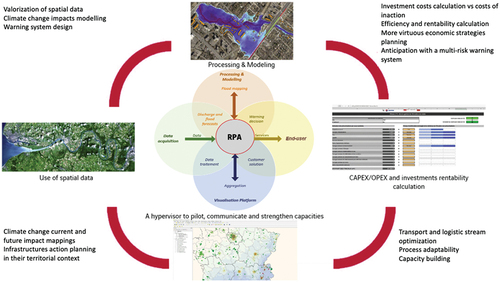
2.1. A geographical information system to visualize climate change impacts

Climate change is not actually creating new hazards, but is contributing to extending their spatial impacts, reinforcing their intensities and worsening their territorial vulnerabilities (Gilbert, 2009; Metzger & D’Ercole, 2009). What is relevant for a decision-maker is to visualize the exposure of their assets over an entire lifecycle or infrastructure concession period to identify critical and vulnerable components and how this vulnerability will be intensified by one or several hazards.

A geographical information system (GIS – Qgis in this project) is the appropriate tool to meet these expectations, as it provides viewing and computational possibilities to process both climate and infrastructure data with a 2D/3D/4D mapping option. With a GIS, it is possible to create the following maps:

• Exposure, which defines the spatial extent of a hazard impact. Exposure can be inferred from Earth Observations data and climatic models and requires downscaling and correction methods to adapt the output results to topographical constraints and land use (Solecki & Oliveri, 2004; Theme, Gobiet & Heinrich, 2012; Figure 2)

  Figure 2. Downscaling principle to adapt climatic models’ outputs to the land-use (Adapted from Willems [2011] in Siwila et al. (2013).

  

Vulnerability of infrastructures and territories. Vulnerability can be defined as ‘the degree to which a system is susceptible to, or unable to cope with, adverse effects of climate change, including climate variability and extremes’ (IPCC & Core Writing Team, 2014,) as shown in Figure 3. Methodologies to assess and map vulnerability are numerous (Alonso, 2021; UNDP, 2017; Armenakis & Nirupama, 2013; Romero-Lankao, Qin & Dickinson, 2012) and need is to evaluate the sensitivity and the adaptive capacity.

Figure 3. Conceptual mapping of vulnerability (Sharma & Ravindranath, 2019).

¹

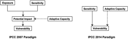
• Cumulative impacts of current and future climate change determine the major risks according to IPCC scenarios. Indeed, climate change risks do not happen independently, but imply complex interactions between hazards. For example during a tropical cyclone several exposure perimeters (wind, riverine floods, flash floods and storm surges) must be combined and reinterpreted through preferential combinations requiring statistical treatments (Figure 4).

  Figure 4. A multi-hazard approach to spatialize complex risks, such as tropical cyclones.

  

2.2. An analytical table to help decision-makers prioritize adaptation solutions

The second tool of RPA is an analytical table with several menus to assess the resilience performance (Figure 5). First, a hierarchical breakdown is made according to the nature of infrastructure: building; road; railway; water and sanitation equipment; bridge; and others.

Figure 5. The resilience performance assessment analytical table allowing the evaluation of climate change impacts.

A sensibility analysis is done for each system and their component with a rating from 1 (single hazard) to 3 (for multiple hazards). An intial score is provided based on a theoretical assessment, without a detailed audit of infrastructure. Second, an analytical framework is filled based on site visits, to capture the potential present and future failures, in terms of safety, users’ comfort and usage, affecting the infrastructure, its equipment and surrounding territory. It provides a second score to adjust the desktop analysis. Another important feature of RPA is that it allows the updating of the risk analysis with new information (such as new climate scenarios or details about the asset), allowing a periodic review of the assets’ vulnerability.

3. A tool to guide decision-makers with adaptation solutions and share climate risks with other stakeholders

Finally, a cost–benefit matrix is completed following a visit to determine the needs in terms of CAPEX/OPEX over time, as well as benefits and co-benefits of resilience improvement.

The tools can be applied to infrastructures at each stage of their lifecycle, as well as to investment projects dedicated to climate change adaptation, urban planning policies, and sustainable transport plans on a national, regional or local scale. For each application, an investment plan is generated considering specific targets: spatial coverage; duration; ability to generate revenue; or conformity with international commitments such as the Paris Agreement and Sustainable Development Goals (SDGs).

RPA can be used as a tool for a common understanding of climate risks to which asset is vulnerable, which is crucial for sharing risks among stakeholders.

The identification of risks and their nature, particularly force majeure risks, allows a better sharing of risks between stakeholders and gives incentives to the infrastructure owner and operator to include adaptation solutions, as they can be responsible for managing these risks. It pushes the private sector to seize opportunities for climate adaptation.

Therefore, cost–benefit analysis included in RPA methodology can be used to compare different adaptation pathways, including a mix of physical solutions to reduce the vulnerability of assets and financial solutions such as insurance policies, contingency plans, risk provisions or tax breaks in the finance model (World Bank Group, 2022). It can then be used by stakeholders to better evaluate the climate risks they are facing and propose another allocation of the risk (between private partners in case of PPPs, insurance companies, public state, investors, debt insurers and so on).

4. An operational and customizable tool

RPA aligns to works of the Global Alliance for Building and Construction (Global ABC), the Coalition for Climate Resilient Investment (CCRI) and the Coalition for Disaster Resilient Infrastructure (CDRI), of which RESALLIENCE is a partner, and is currently used by several customers of RESALLIENCE.

This article demonstrates the application of RPA to a small Caribbean island. This territory is strongly dependent on its critical infrastructure for importing essential supplies and exporting goods. With most of its population and critical infrastructure located along the coastline, this state has been affected hard by two hurricanes, Erika (2015) and Maria (2017). The last cyclone caused the destruction of 20% of the buildings and damage to the remaning 80%. A resilience performance assessment was conducted to support the national resilience strategy and optimize future investments.

This analysis is available through a secured web page, giving access to a hypervisor of current and future impacts of climate change. Multi-hazard maps have been developed to assess the impacts of complex hazards, such as hurricanes. A multicriteria analysis identified the extreme risk scenarios for each hazard. They are then combined in a correlation matrix to evaluate the different combinations of event occurrence, e.g., the simultaneous occurrence of high wind and floods, high wind and storm surge, or floods and storm surge (Figure 6).

Figure 6. Exposure mapping of multiple hazards to identify most exposed parts of the island to complex risks such as hurricanes.

Note: The hypervisor content cannot be shown in its entirety due to a confidentiality agreement.

Vulnerability maps are calculated for a 350 m² mesh. The density of human and environmental assets as well as critical infrastructure assets has been considered in the GIS, with an analysis of their statistical variance through a principal component analysis (Figure 7).

Figure 7. Mapping of vulnerability from multiple hazards to identify the most vulnerable sectors of the island.

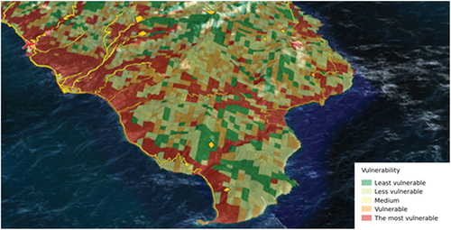
In this case study, the resilience performance of current and future investment projects has been assessed. More than 300 projects were analysed through surveys with institutional stakeholders and private decision-makers. Each project was rated considering its ability to make revenue streams, its spatial coverage, its duration and its capacity to reduce risk in compliance with international and national commitments (SDGs).

On the platform a flag is used to mark each project to analyse the investment scoring with the vulnerability of the critical infrastructures. The combination between these two layers of information allows identification of the sectors where projects are missing or needed to enhance infrastructure resilience (Figure 8).

Figure 8. Localization of current and future investment projects facing island territorial vulnerability.

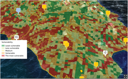
5. Decision support tool to guide adaptation solutions and climate risk sharing with other stakeholders

The RPA tool allows the assessment of both the internal and external risks to which the project is subject. In most cases, external risks are covered by the public sector, while internal risks can be covered by concessionaires through capital or insurance coverage (particularly in PPP projects). Therefore, RPA provides common understanding among stakeholders about the climate risks to which the asset is vulnerable, which is key for sharing risks among stakeholders. Another important feature of RPA is the convenience of updating risk analyses with new information (such as new climate scenarios or more asset details) for a periodic review of assets’ vulnerability.

Identification of risks and their nature, particularly force majeure risks, allow a better sharing of risks among stakeholders and gives incentives to the infrastructure owner and operator to include adaptation solutions as they are responsible for managing these risks. It encourages the private sector to harness climate adaptation.

Therefore, cost–benefit analysis in RPA compares different adaptation pathways, including a mix of physical solutions to reduce the vulnerabilities of asset and financial solutions such as insurance, contingency plans, risk provisions or tax breaks in the finance model (World Bank Group, 2022). The results enable stakeholders to better evaluate the climate risks they are facing and propose efficient allocation of the risk (among private partners in the case of PPPs, insurance companies, public state, investors, debt insurers and others).

6. Conclusion

The proposed solution presented in this article aims at helping decision-makers to make decisions which increase climate resilience of the territory and/or the assets they manage or own considering multiple criteria. To solve this problem, the article presents an innovative methodology, termed resilience performance assessment (RPA), that combines financial, geographic and climate modelling as well as dashboards to help decision-makers better manage and share climate risks. This innovation allows efficiency and balance between physical and financial adaptation solutions for climate change across full infrastructure life cycles and territories. RPA consists of two operational tools: a geographical information system, allowing a clear and comprehensive visualization of climate change impacts; and an analytical table to support stakeholders in prioritizing adaptation strategies, including physical and financial solutions. The climate model has been developed using dynamic downscaling algorithms up to a 1km x 1km spatial resolution.

The RPA can be used to evaluate climate change adaptation risks in investment costs, as well as operation and maintenance costs of infrastructure. It provides dedicated metrics and analysis to assess the capabilities of internal and external investment managers for incorporating adaptation risks before investment service providers (financial analysts, consultants, brokers, research firms, rating companies and others). It can also be used to provide training and capacity-building for investment professionals.

Disclosure statement

The DRI Technical Conference 2022 was sponsored by CDRI, along with editorial work of the Conference Proceedings. However, CDRI did not influence the research, data, findings, and views presented in the research papers.

Changing the valuation paradigm to promote adaptive and resilient infrastructure investment: connecting insurance concepts and valuationCONTACT David Espinoza [email protected]

ABSTRACT

Despite irrefutable evidence of a looming climate crisis that could lead to significant environmental disasters, (i) climate change risks are not sufficiently captured in the value of vital assets (e.g., power plants, roads, dams) and (ii) investors have not modified their approach to planning, valuing and financing such assets to account for the considerable physical risks posed by climate change. Thus, the benefits of incorporating features to make assets resilient to climate change are not fully captured in financial analyses. Why? The mechanics of standard valuation approaches such as discounted cash flows (DCFs) exacerbate our innate human predisposition to short-term thinking by emphasizing short-term revenues and expenditures and neglecting long-term ones. Furthermore, these outdated techniques are incapable of properly valuing the flexibility provided by adaptive infrastructures to respond to the changing climate, thus neglecting (and undervaluing) management’s ability to make changes as uncertainty gets resolved. Given the uncertainty of future climate impacts, a timely implementation of flexible and adaptive infrastructure will be paramount for optimizing the allocation of limited financial resources. Despite the benefits of investing in resilience and adaptation, DCF’s inability to account for climate change risks in a financial analysis makes it hard to justify investing in such features. The urgency of pivoting to a robust model like the decoupled net present value (DNPV) is growing. Like insurance products, DNPV defines all risks (including climate change) as loss potentials and quantifies them in monetary terms (the cost of risk). Risk has a cost whether we pay for it or not.

KEYWORDS:

• DNPV
• resilience and adaptation
• cost of risk

1. A brief history of discounted cash flow (DCF)

To calculate the economic value of assets, standard approaches such as discounted cash flow (DCF)¹ require forecasting uncertain cash flow (revenues and expenses) over the asset life and calculating the magnitude of the discount to account for investors’ risk and time preferences. Most investors are risk averse and prefer cash flows that are certain over those that are uncertain (i.e., riskier). Likewise, most people confer a higher value on goods received sooner than those received later – the further into the future, the lower their value. When the goods being considered are money, the time-preference effect is called the time value of money (TVM). Hence, both risk and TVM reduce (i.e., discount) the value of future cash flow. How much should future cash flow be discounted? Sharpe (1964) supposedly answered this question with the development of the capital asset pricing model (CAPM), which was built upon modern portfolio theory (MPT), which assumed investors are rational, markets are efficient and utility theory is valid (Markowitz, 1952). In his seminal work, Markowitz introduced price volatility (i.e., dispersion around the mean of stock prices) as a proxy for risk. Since then, risk and volatility have been used interchangeably, and all financial decisions are assumed to fit Markowitz’s MPT formulations. This modern definition of risk made it easy to compare traded stocks – higher volatility implies higher risk – losing in the process the everyday meaning of risk (i.e., the fear of a loss).

A good proxy for TVM is risk-free rates (i.e., the theoretical rate of return on an investment with zero risk). Risk-averse individuals purchase government-issued bonds in exchange for a stream of future certain cash flows. For risky assets, CAPM provides investors with a prescriptive framework for calculating a risk-adjusted discount rate: the sum of a risk-free rate plus an equity risk premium. Conceptually, this easy-to-grasp concept of adjusting risk-free rates to account for risk captured the risk-averse nature of investors who would pay less for a future risky positive cash flow than for a riskless one. However, by adding a risk premium to the risk-free rate, multiple incorrect assumptions are implicitly made: (i) risk and TVM are described by the same exponential function; (ii) the effect of risk and TVM are fully interchangeable; (iii) risks are source independent and increase with time; and (iv) risk has the same effect for revenues or expenses.²

Although risk and TVM are inexorably intertwined in any investment, risk and time preferences are not the same and should be separated when evaluating investment opportunities. Work on capital budgeting and valuation of investments in real assets assumed that risks and TVM evolved consistently with CAPM. This assumption continued despite the ensuing criticism regarding its validity and predictive capabilities (e.g., Ross, 1976). Unsurprisingly, attempts to capture physical risks (e.g., climate change) also followed this trend (i.e., adjusting risk-free rates). Because DCF creates a pernicious time-bias effect, its application makes it difficult to assess the effect of investing today to protect real assets against future physical risks objectively. Unfortunately, CAPM’s simple predicament of adding a risk premium to the risk-free rates has so far prevailed.

2. Certainty equivalent method: a failed attempt

Although the scientific and engineering communities have made significant advances in forecasting future climate impacts on physical assets, the significant time-bias effect introduced by DCF approaches neglects the evident benefits that resilient and adaptable infrastructures provide, making it difficult for managers to justify investing in such features. Increasing awareness of the importance of solving this pressing issue has made practitioners and academics start questioning the fundamental tenets of MPT (e.g., investor rationality, efficient market hypothesis, utility theory) and, with that, the applicability of DCF (e.g., Lukomnik & Hawley, 2021).

The quickest way to address the DCF limitations is to separate TVM and risk, giving investors greater flexibility for risk modelling. Ironically, this was proposed shortly after CAPM was introduced. Robichek and Myers (1966) indicated that adding the TVM and risk effects in a single parameter was not appropriate and proposed the certainty equivalent method (CEM). The CEM consists of estimating expected cash flows, reducing them to account for risks, and discounting these reduced cash flows using risk-free rates. Investors need to assess the riskiness of the cash flows and specify equivalent amounts that would make them indifferent between risky and riskless cash flows. The CEM did not provide protocols on how to calculate certainty equivalents consistently, which made it difficult for CEM to gain popularity among practitioners despite its promise.

3. The cost of risk: reconnecting losses with everyday meaning of risk

Multiple studies indicate that investors are averse to losses, not volatility (Kahneman & Tversky, 1979). An individual’s loss-averse nature was recognized by the French mathematician de Moivre over 300 years ago, when risk was simply referred to as the possibility of harm, injury or loss. Furthermore, the idea of estimating loss exposure can be traced back to the ancient Babylonians. The code of Hammurabi describes an arrangement that would be characterized today as marine insurance. To finance shipments, merchants obtained loans that included monetary premiums to protect them from being liable for loan repayment if the vessels failed to reach their destinations. These ancient monetary premiums can be described as the cost of risk. Collecting premiums for taking risks is familiar to the insurance industry and the public who buy insurance products.

Similar to insurance products, monetary premiums can be objectively calculated from the downside distribution of the cash flows independent of the investor’s feelings about risk. This provides investors with a much-needed prescriptive and robust framework to estimate certainty equivalents consistently. Interestingly, buying insurance protection against certain risks is common in most businesses. For instance, farmers often purchase insurance to protect their income should their crops be destroyed by natural disasters (i.e., physical risk) or should the price drop (i.e., market risk). Furthermore, estimating costs of typical insurable risks and keeping these risks in house is a well-established practice of mid- to large-size corporations today (e.g., self-insurance, captive insurance). All these cases share common elements: once risks are identified, the cost of risks is calculated in monetary terms to better understand the financial risk exposure, and said risks are either transferred to third parties (e.g., insurance providers, business partners) or assumed by owners. Inexplicably, although investors and owners embrace the cost-of-risk concept for insurable risks, they commonly dislodge the connection between risk and losses when dealing with project risks and use risk-adjusted discount rates instead. This practice obscures investors’ exposure to losses.

Considering risks as costs to projects is a natural progression from buying insurance for specific, insurable risks and self-insuring others. In the cost-of-risk concept, investors are likened to insurance companies in that they need to calculate monetary premiums to describe risks and assess whether the calculated premiums are appropriate compensation for bearing the identified cash-flow downside risks. Assessing monetary values to all identified risks will allow investors to reconnect potential losses with the sources of risk, evaluate risk effects on cash flows, select appropriate risk-management measures, and allocate capital more efficiently. Investors would need to quantify the cost of risk for each identified risk exposure using market data, industry databases and expert opinions. This added work allows investors to better understand their true risk exposure and eliminates the DCF’s time-bias effect.

In summary, risk should be redefined – away from the MPT’s risk definition (i.e., volatility) – back to its original intuitive and useful definition: the fear of loss. The estimate of the investment’s loss exposure (i.e., cost of risk) can be calculated using the cash flow’s probabilistic distribution. From this loss perspective, risk means that revenues could be lower than (and/or expenses higher than) expected. Regardless of the actual mechanics, the cost of risk should reduce the value of positive cash flow (revenue) and make negative cash flow (expenditure) more expensive. This is accomplished by subtracting the estimated cost of risk from the expected cash flow. Because cash flows are modified to account for risks, they can be discounted using the risk-free rates.

4. The decoupled net present value (DNPV) method

The DNPV method, a valuation framework developed for infrastructure investments (Espinoza & Morris, 2013), has the desired features described above, namely: (i) the separation of risk and TVM à la CEM; (ii) the use of the cost-of-risk concept to estimate certainty equivalents cash flows; and (iii) the use of risk-free rates to account for TVM of cash flow. DNPV captures the infrastructure’s exposure and vulnerability to physical risks (e.g., climate change) and other nonmarket risks (e.g., political). Regardless of the source (market, nonmarket), the cost of risk is calculated in the same manner (i.e., the potential loss exposure for a given risk). There is no need to adjust the discount rate to account for risk because all risks are incorporated in the cash flow. The ability of DNPV to deal with a variety of risks regardless of their source makes it uniquely suitable to evaluate long-term infrastructure assets.

Under DNPV, each risk has a cost. Like insurance premiums, these costs negatively impact cash flow. The advantage of using the cost-of-risk concept is that it makes certainty equivalent revenues smaller and certainty equivalent expenditures higher.³ Because risks associated with a project are directly accounted for in the cash flows, the net certainty equivalent (i.e., riskless) cash flows can then be discounted using term-appropriate risk-free rates.⁴ This is summarized in Equation (1)(1) $\mathrm{D}\mathrm{N}\mathrm{P}\mathrm{V}=\sum _{t=0}^T\frac{V_t-E_t-R_t}{{\left(1+r\right)}^t}$(1) below.

(1) $\mathrm{D}\mathrm{N}\mathrm{P}\mathrm{V}=\sum _{t=0}^T\frac{V_t-E_t-R_t}{{\left(1+r\right)}^t}$(1)

where T is the asset life, $\underset{t}{V}$ and $\underset{t}{E}$ are the expected cash flows (revenues and expenditures, respectively), R_t represents the costs of risks at time t, and r is the risk-free rate to account for TVM. Data can be compiled in repository databases conducive to data analytics techniques that improve estimates of costs for similar risks. Unlike insurance premiums, the cost of risk does not render the project riskless. It only values the identified investment risks and incorporates them in the valuation process. Some identified risks may be transferred to insurance providers, but investors will retain most project risks. Thus, the risk of the project becoming unfavourable (i.e., obtaining lower revenue or spending more than anticipated) is borne by the investor. Thus, investors are likened to insurance providers with the cost of risk representing their compensation for taking on such risks.

Since DNPV was first introduced, it has been implemented for multiple applications, including agriculture (e.g., López-Marín, Del Amor & Brotons, 2020), renewable energy (e.g., Espinoza & Rojo, 2015), transportation (Nguyen, Almarri & Boussabaine, 2020), oil & gas (Ponomarenko, Marin & Galevskiy, 2022), solid waste (Shimbar & Ebrahimi, 2017), and others. As demonstrated by these applications, non-market risks can be accounted for through judicious development of probability density functions that best describe the risks under consideration using data analytics along with relevant science. For cases where observed market prices are available, the cost of risk can be calculated using the observed pricing data (e.g., futures). Thus, DNPV can easily incorporate climate risk by considering climate science, data analytics and engineering quantitative risk assessments to evaluate the impact of resilience and adaptation features of infrastructures.

5. Chronic and acute risks

Climate-change risks are often classified as (i) chronic risks to refer to permanent changes of the probability distribution captured by a change in the expected value of cash flows; and (ii) acute risks to refer to the increase in the low-frequency (tail) events that translate to an increase in the standard deviation of the cash flows. Climate change risks usually affect both.

Because standard valuation methods are based on MPT’s principles, DCF approaches only account for market risks: the effects of nonmarket risks (e.g., physical risks) are not included. However, since DCF uses expected values, the effects of physical risks can be readily extended to capture changes in expected values (i.e., chronic risks). The same cannot be done for acute risks. There is no straight connection between physical risks and discount rates. This invariably leads to heuristic arguments to justify higher discount rates, thus exacerbating the time-bias effect that minimizes long-term negative effects of climate change.

Climate change introduces a significant downside (acute) risk that translates to a material change of expected values. Since DNPV uses probability distributions to estimate cash flows’ expected values and loss exposures (downside potential), both chronic and acute risks are properly captured in the financial analysis. Because potential losses are measured as shortfalls from expected values (Figure 1a), a pure shift of probability distributions would not result in a change of the downside potential (i.e., cost of risk remains unchanged). Contrarily, an increase in the cash flow variability would result in larger potential losses even if expected values remain unchanged (Figure 1b).

Figure 1. Illustration of climate risk classification (for revenues).

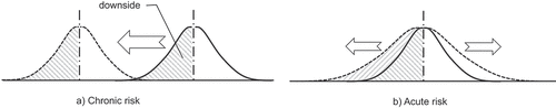
6. Valuation example

For illustration purposes, a simple example is presented as Table 1, showing both NPV and DNPV calculations. The example represents an initial capital expenditure (CAPEX) of US$110 million at a coastal industrial facility that would generate annual revenues of US$25 million with an annual operating expenditure (OPEX) of US$10 million (in today’s dollars), netting US$15 million annually for 30 years. To facilitate the discussion, let’s assume that the corporation negotiated an agreement that secures its net revenue for 30 years. Let’s further assume that the corporation cost of capital is 5% (net of inflation), which is used to calculate the NPV for the cash flows in Row E yielding US$120.6 million.

Table 1. Valuation example comparing NPV and DNPV estimations (US$).

Year	0	1	2	…	10	…	30
A. Revenue		$25.00	$25.00		$25.00		$25.00
B. OPEX		$10.00	$10.00		$10.00		$10.00
C. Net revenues		$15.00	$15.00		$15.00		$15.00
D. CAPEX	-$110.00
E. Cash flows (CF)	-$110.00	$15.00	$15.00		$15.00		$15.00
F. NPV (5%)	$120.60
G. Expected (chronic) CF	-$110.00	$14.40	$14.40		$14.40		$14.40
H. Climate risk (acute risk)	-	$2.40	$2.40		$2.40		$2.40
I. Decoupled CF	-$110.00	$12.00	$12.00		$12.00		$12.00
J. DNPV (1.02%)	$302.20

We also assume that the industrial facility’s location can be affected by severe flooding due to climate change with an annual probability of occurrence of 4% that might result in a year-long shutdown (resulting in a US$15 million of loss net revenues) and equipment damage to the sum of US$45 million. The potential shutdown effect (chronic risk) is included in the NPV by revising the cash flows’ expected value to US$14.4 million (0.96× US$15 million +0.04× US$0). Classical NPV would dictate to discount the revised cash flows using the cost of capital (i.e., 5%) yielding a value of US$106.1 million. Let’s also assume that the owner has the option to make the facility essentially immune to flooding by investing an additional US$10 million (increasing CAPEX in Row D to US$120 million) to avoid the potential US$60 million loss due to flooding. Since traditional NPV cannot consider contingent liabilities, the additional investment of US$10 million would reduce the NPV down to US$96.1 million.

Under DNPV, the US$60 million contingent liability (acute risk) results in an annual cost of risk of US$2.4 million (4%×US$60 million), which is included in the analysis (Row H). Because risk is considered, the resulting cash flows (Row I) can be discounted using a risk-free rate. For this example, the quoted risk-free 30-year inflation protected rate is 1.02% (1 September 2022). The DNPV for the facility without the climate-resilient features is US$198.8 million. By investing US$10 million, the annual US$2.4 million liability (Row H) is removed, and the expected annual cash flow (CF) is again US$15 million resulting in a DNPV of US$276.0 million. As shown in this example, the mechanics of DNPV are relatively straightforward to implement, and the connection between risk and resilience is clear.

7. Conclusions

Combining concepts from CEM and insurance (cost of risk), DNPV is presented as a solid valuation model. Risk is decoupled from the TVM and accounted for in the numerator as a cost to the project calculated based on the cash flow probability distribution regardless of the risk source. This allows for consistent and transparent risk pricing. The concept of cost of risk is used to price the risk associated with obtaining lower revenues (e.g., revenue losses due to shutdown) or incurred in higher expenditures (asset damage due to flooding) than originally expected. These costs of risks are treated as ‘real’ costs to be subtracted from the expected cash flows. Because the risks associated with the project are accounted for by the cost of risk, the reduced cash flows can be discounted using a risk-free rate, which relieves the investors of the task of guessing the ‘appropriate’ discount rate. The cost of risk represents the minimum compensation that the investor should be paid to carry the identified risks, and, in some cases, they may be replaced by actual quoted insurance products. DNPV provides a bridge between the investment and insurance industries. A judicious combination of insurance products, self-insurance and risk-sharing mechanisms can result in optimal decisions.

Disclosure statement

The DRI Technical Conference 2022 was sponsored by CDRI, along with editorial work of the Conference Proceedings. However, CDRI did not influence the research, data, findings, and views presented in the research papers.

Flood disaster risk assessment for critical transportation infrastructure under climate changeCONTACT Kapil Gupta [email protected]

ABSTRACT

Major cities of the world such as Sydney, New York, London, Durban, Mumbai, Chennai and Bengaluru were disrupted by severe rainfall events during 2021–2022. These events overwhelmed the capacity of existing drainage systems, resulting in severe flooding and disruption to the critical transport infrastructure (road, rail and air) of many cities around the world. Climate change is now a harsh reality, with increased rainfall occurring over shorter intervals of time. A flood vulnerability and mitigation assessment for flood prone areas was carried out for the Mumbai International Airport and the Mumbai suburban system of Indian Railways for extreme rainfall scenarios, including a 20% increase in the design rainfall considering the scenario of climate change. This paper presents an overview of the problem, the flood risk assessment methodology adopted and recommendations on adaptation and mitigation measures to reduce the flooding of the airport runway and railway premises to levels well within the safe operating conditions. The methodology has been successfully implemented for the Mumbai International Airport, while the model simulations indicated that the recommended adaptation and mitigation measures will enable Indian Railways to continue train operations even under extremely severe rainfall in the future.

KEYWORDS:

• Flood disaster risk assessment
• resilient transport
• infrastructure
• Indian Railways
• Mumbai airport

1. Introduction

Major cities of the world such as Sydney, New York, London, Durban, Mumbai, Chennai and Bengaluru were disrupted by severe rainfall events during 2021–2022. These events overwhelmed the capacity of the existing drainage systems, resulting in severe flooding and disruption to the critical transport infrastructure (road, rail and air) of many cities around the world. Climate change is now a harsh reality, with increased rainfall occurring over shorter intervals of time. Severe flooding events in monsoon usually result in disruption to rail and road transport in urban centres in India. Airports are critical infrastructure, as they are the only alternative for providing rescue and relief material, as well as for intercity travel, during severe flooding. It is therefore of the utmost importance that these are made flood proof by providing efficient drainage for a much higher rainfall intensity and by using best management practices like holding ponds (NDMA, 2010).

A flood vulnerability and mitigation assessment for flood prone areas was carried out for the Mumbai International Airport as well as the Mumbai suburban system of Indian Railways for extreme rainfall scenarios, including a 20% increase in the design rainfall, taking into consideration the scenario of climate change (DEFRA/Environment Agency, 2005). This paper presents an overview of the problem, the flood risk assessment methodology adopted and the recommended mitigation measures to reduce flooding on the airport runway and railway premises to levels well within safe operating conditions. The methodology has been successfully implemented for the Mumbai International Airport, while the model simulations indicated that the recommended mitigation measures will enable Indian Railways to continue train operations even under extremely severe rainfall in the future.

1.1. Background

On 26 July 2005, due to extremely heavy rainfall in Mumbai (190 mm in one hour, 707.6 mm in 7 hours and 865.5 mm in 12 hours; Figure 1), the complete airport area including runways, parking bays and external airport access roads were submerged and all air traffic was suspended for more than 48 hours.

Figure 1. Hourly storm hyetograph from 26 July 2005 at 2.30pm to 27 July 2005 at 2.30am with a period of high intensity between 2.30pm and 9.30pm (IST).

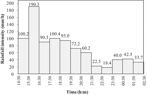
One of the main reasons for the flooding of the airport was the overflowing of the Mithi River upstream of the river culvert passing under the main airport runway 09–27 (Government of Maharashtra, 2006). The old 27 m wide and 382.50 m long culvert was constructed for the undeveloped catchment conditions, but the contributing catchment area of 4929 hectares has undergone rapid change in land use pattern and is now mostly urbanized and densely populated with a population of 1.05 million people. All flows in the catchment discharge into the Mithi River, which then passes under the airport through this culvert. An earlier study by the authorities of the airport flooding problem had proposed diversion of the river from outside the airport area, but the topography and human settlements (> 10,000) did not make this viable. Hence, this study was carried out to identify a practical solution with adaptive pathways. The major challenge was to provide an additional waterway without closing the single runway. This paper describes the comprehensive hydrologic and hydraulic simulations carried out in this study to find an implementable solution.

2. Case study 1: Mumbai airport catchment description

Mumbai International Airport is spread over an area of 610 ha with the capacity to handle 0.11 million passengers per day and air traffic of 912 flights per day from a single runway (09–27). The Mithi River catchment is the largest catchment (7265 ha) in Mumbai (Figure 2), out of which 4929 ha contributes to the flow through the airport culvert passing under the main runway (09–27). The overall objective is to meet future aviation demand in a safe, secure and efficient manner, at a reasonable level of service, with the need to improve infrastructure and increase capacity within the application of mandatory ICAO and DGCA regulations. While Mumbai airport has another runway, 14/32, this cannot be used simultaneously as it cuts across the main runway (09–27), a full parallel taxiway system is lacking and other obstructions are present.

Figure 2. Mithi River catchment and Mumbai International Airport.

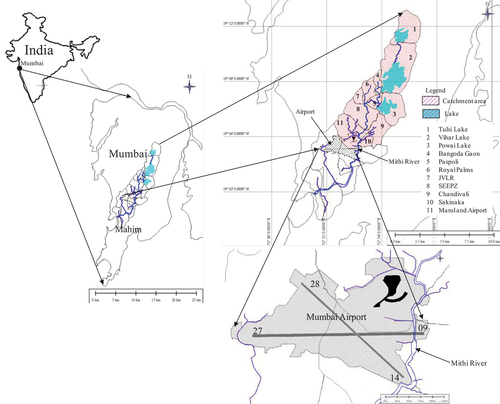
The river elevation varies from 37.98 m (MSL) at the highest point (downstream of Vihar Lake) to −2.50 m (MSL) at the lowest point (Mahim causeway), as shown in Figure 3.

Figure 3. Longitudinal profile of Mithi River.

Source: Government of Maharashtra, (2006).

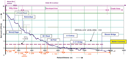
2.1. Methodology

The overall methodology is shown in Figure 4.

Figure 4. Overall methodology.

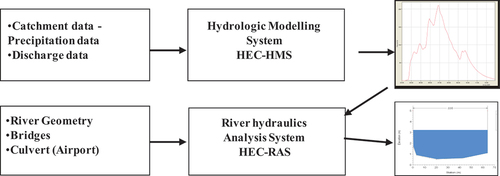
The analyses for both the airport and the railway studies have been carried out using the US Army Corps of Engineers Hydraulic Engineer Centre’s Hydrologic Modelling System (HEC-HMS, 2010a) and River Analysis System (HEC-RAS, 2010b) to determine the water levels for the design flood and possible submergence for various culvert waterway alternatives. The calibration of the HEC models was carried out using the observed severe rainfall events of 4 July 2009, 14 July 2009 and 3 July 2010.

Rainfall intensity of 100 mm/h (corresponding to the 1 in 100-yr return period) has been used for hydraulic design as recommended by the Fact-Finding Committee set up by the Government of Maharashtra (Government of Maharashtra, 2006). The 1 in 100-year design storm for critical infrastructure has subsequently been incorporated in the CPHEEO Urban Drainage Manual (CPHEEO, 2019). In addition, to consider climate change effects, the design rainfall has been increased by 20% (DEFRA/Environment Agency, 2005). Hence, the peak discharges from the sub-catchments have been estimated for a rainfall intensity of 120 mm/h. The peak discharge has been estimated using HEC-HMS 3.4 and used in the river analysis model HEC-RAS 4.1 to compute the corresponding depth of flow at specific cross-sections.

2.2. Estimation of flow depth for the old culvert (27 m wide with three bays)

Water levels have been computed for the peak flow of 1088 m³/s using HEC-RAS at the old culvert at 27 m wide with 3 bays of 9 m each and 4.1 m of depth. It is seen that with the 27 m wide culvert scenario, a water level of 10.230 MSL occurs at the u/s of airport culvert with backwaters reaching up to 10.400 MSL at upstream point (White Bridge) and submerging the main runway. Simulations were carried out to determine the size of the additional channel, so that the water level is below the soffit level of the main runway. It was found from the analysis that the required waterway is 47 m for design flow of 1088 m³/s. However, the airport operations group indicated that the widening of the old 27 m culvert under the main runway was not possible, as this would result in an inadequate take-off length for the aircraft. It was therefore decided to consider the location of the additional culvert at the extreme east end of the runway (Figure 5).

Figure 5. Proposed widening of the existing culvert.

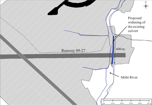
Also, instead of a straight channel, a curved culvert (Figure 6) was provided so that the required runway length was available for aircraft operations during the construction phase.

Figure 6. Final curved box culverts provided.

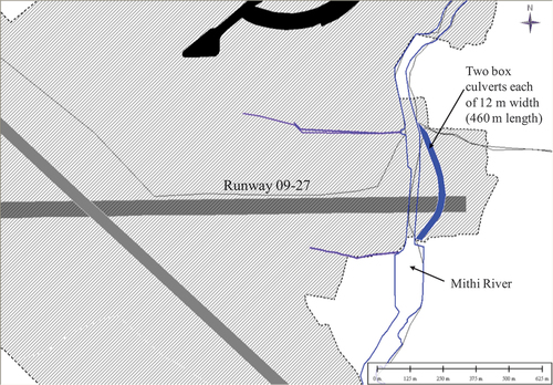
The hydraulic analysis was repeated for the relocated curved culvert, and it was seen that due to the bifurcation of the 20 m channel into two sections of 10 m each, the water levels at the culvert inlet were found to be higher than the soffit of the culvert under the runway (Figure 7). Hence, to maintain the water level below the runway culvert soffit, the width of the two box culverts were determined as 12 m each. These dimensions were found adequate to discharge the design flood without submerging the main runway.

Figure 7. Water levels for widening two culverts and an additional culvert.

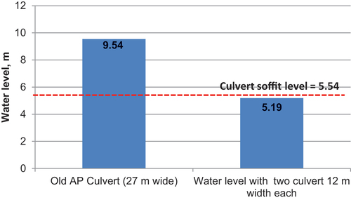
These works were executed without any disturbance to aircraft operations and completed in June 2012. The airport is functioning without the threat of disruption from severe flood events.

3. Case study 2: Mumbai suburban railway system

A flood vulnerability and mitigation assessment has been carried out for a severe flood prone area on the Mumbai suburban railway system, namely the Kurla–Lokmanya Tilak Terminus complex on the Central Railway. The objectives of the assessment were to:

1. Analyse the existing drainage system and its constraints; and

2. Recommend feasible mitigation and adaptation measures.

3.1. Methodology

The methodology for the case study area consisted of the study of previous reports, reconnaissance visits, hydrologic analysis, mathematical simulation using the HEC-RAS model, evaluation of various alternatives and recommendation of mitigation measures within the limitations of the site conditions and data availability.

The hydrologic analysis described here to compute the peak discharge for the catchments has been carried out for a 120 mm/h rainfall intensity (1 in 100-yr rainfall plus 20% extra for climate change), which has worked successfully for the airport area. The peak discharge has then been used to compute the water levels for the existing situation as well as for the proposed mitigation measures using the HEC-RAS simulation model. After the evaluation of various alternatives, mitigation and adaptation measures have been recommended which resulted in the reduction of simulated water levels to permissible levels under the scenario of heavy rainfall along with the climate change scenario in the case study area.

Two holding ponds as shown in Figure 8 have been identified in the Kurla-LTT Railway complex: HP1 with a volume of 32,000 m³ (16,000 m² area with proposed water depth 2.0 m + 0.3 m freeboard) and HP2 with a volume of 72,000 m³ (36,000 m² area with proposed water depth 2.0 m + 0.3 m freeboard), giving a total volume of 104,000 m³ to mitigate the flooding.

Figure 8. Proposed holding ponds in the Kurla-LTT area, Mumbai, India.

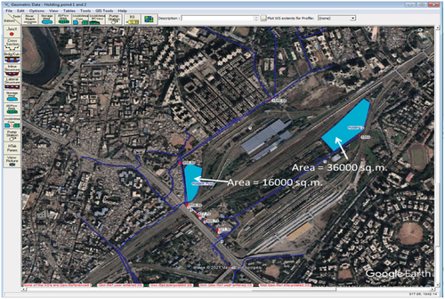
During the site visit, a divide wall/weir was seen to be situated between the outlet of the additional culverts and the Carshed Nallah south of the Railway Colony, which was observed to be impeding the flows from the pipe culverts. Hence, removal of the weir wall could create additional pathways for the floodwaters and reduce the water levels in the culverts. Analysis has been carried out to determine the water levels with and without the weir wall for various rainfall scenarios using the HEC-RAS model; these are shown in Figure 9. In addition, analysis has been carried out to determine the impact of the holding ponds with and without the weir wall for various rainfall scenarios, and these are also shown in Figure 9. It can be seen that when two holding ponds are provided, there is a significant reduction in water level by 2.29 m for 120 mm/h rainfall.

Figure 9. Reduction in water levels due to the proposed mitigation measures.

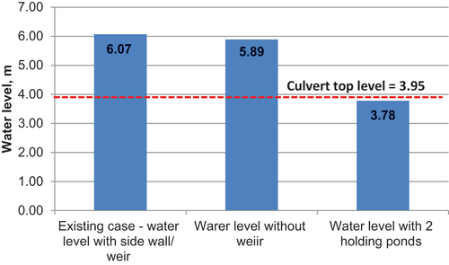
4. Summary and conclusions

The main focus of the study has been to determine the adaptive pathways within the boundary conditions of the airport and railway premises for the design flood resulting from rainfall (120 mm/h) corresponding to a 1 in 100-yr return period and an additional 20% for climate change. The hydrologic and hydraulic modelling was carried out using HEC-HMS and HEC-RAS. For the airport, the additional waterway was determined such that the high flood level remains below the runway culvert soffit and permits airport operations under severe rainfall including climate change. Considering the site conditions and airport traffic, two additional curved culverts of 12 m each were found adequate to discharge the design flood. The waterway under the airport runway has now been increased from 27 m to 51 m and the airport is functioning without the threat of disruption from severe flood events.

For the railway case study, the simulations show that the provision of the two holding ponds and removal of the weir wall would significantly reduce the water levels over the tracks and allow the operation of the railways for the 1 in 100-yr 120 mm/h rainfall.

Disclosure statement

The DRI Technical Conference 2022 was sponsored by CDRI, along with editorial work of the Conference Proceedings. However, CDRI did not influence the research, data, findings, and views presented in the research papers.

‘InfraRivChange’: a web application to monitor river migration at sites of critical bridge infrastructure in the PhilippinesCONTACT Richard J. Boothroyd [email protected]

ABSTRACT

Shifting rivers, particularly with high migration rates, represent a geomorphic hazard at sites of critical bridge infrastructure. Conventional attempts to map and measure shifts in the position of river channels usually requires the manual digitization of riverbanks from satellite imagery using Geographic Information Systems (GIS) – a time-consuming process only feasible at a limited number of bridge sites using a small selection of satellite images. As part of the CDRI Fellowship, the authors leveraged the cloud computing platform Google Earth Engine (GEE) to substantially upscale analyses using Earth observation (EO) data. Focusing on the Philippines, they designed a user-friendly web application for technical and non-technical users to monitor the relative risk of river migration at sites of critical bridge infrastructure by analysing thousands of satellite images. ‘InfraRivChange’ uses openly accessible satellite imagery from Landsat (30 m spatial resolution) and Sentinel (10 m spatial resolution) to quantify river channel changes at bridge sites. The study demonstrates the web application at test sites and suggests use-cases relevant to disaster resilient infrastructure. As a low-cost approach for monitoring shifting large rivers in the vicinity of infrastructure, InfraRivChange can be incorporated into bridge monitoring systems (e.g., as a component of bridge stability assessments) and inform the design and placement of future infrastructure. They envision that InfraRivChange can be applied to additional forms transport infrastructure adjacent to rivers (e.g., road and rail) and extended to other dynamic riverine settings.

KEYWORDS:

• Critical bridge infrastructure
• transportation
• geomorphic hazards
• river hazards
• satellite imagery

1. Introduction

The Philippines is among the most vulnerable countries in Southeast Asia exposed to the impacts of climate change (Yusuf & Francisco, 2009) and consistently ranks as one of the countries most affected by extreme weather globally (Eckstein, Künzel & Schäfer, 2021). Climate change is impacting the magnitude and frequency of extreme flood-generating storms (Eccles, Zhang & Hamilton, 2019; Tolentino et al., 2016) and a high proportion of the population are exposed to hazards arising from fluvial flooding and erosion (Smith et al., 2019). Hydrometeorological hazards such as floods and rainfall-triggered landslides (Abancó et al., 2021; Catane et al., 2012) damage critical infrastructure, especially transport infrastructure like bridges, roads and railways.

River bridges are vulnerable nodes in transport and utility networks, and are more exposed to hydrometeorological hazards than other infrastructure assets (Pregnolato, 2019). Their damages or destruction result in high socio-economic costs (Enke et al., 2008). River migration and associated scour represents a systemic hazard at sites of critical bridge infrastructure. In the Philippines, where exposure to flooding and geomorphic risks are considerable (Dingle et al., 2019), recent expansion of infrastructure developments (World Bank, 2018) warrants quantification of river migration in the vicinities of large bridge assets. Road networks in the Philippines handle 90% of passenger and 50% of freight transportation (Vallejo, 2015) and are vital for linking rural communities (Olsson, 2009), but considerable damages are recorded during hydrometeorological events. As climate change increases the frequency and magnitude of typhoons and storms in tropical regions, it will further undermine the stability of bridges, levees and other infrastructure (Eccles, Zhang & Hamilton, 2019).

To address river migration in relation to transport infrastructure, Earth observation (EO) data can be used to monitor river channel change in the vicinity of bridges. This information can improve understanding of river behaviour and help in the design of mitigation measures for transport infrastructure. Capturing satellite imagery at predictable time intervals is a major advantage for mapping changes in river channels (Carbonneau & Piégay, 2012), and for very large river systems, aerial or satellite remote sensing systems can be the only way to observe and quantify planimetric morphology (Gilvear & Bryant, 2016). Hazard monitoring from satellite imagery has been completed around large bridges on the Padma River, Bangladesh (McLean et al., 2012) and Ayeyarwady River, Myanmar (Oo, Kyi & Zin, 2019). Although EO data supports a range of disaster risk reduction activities, the large volumes of data available to risk practitioners can be challenging to handle and process.

Technological advances in digital infrastructure, increased computing power and data storage capabilities have given rise to cloud computing platforms, providing on-demand access to high-performance computing facilities without a need to own and maintain physical hardware (Sudmanns et al., 2020). An example is Google Earth Engine (GEE), a cloud computing platform for planetary-scale geospatial analysis (Gorelick et al., 2017). GEE holds a substantial data catalogue of EO data, providing near real-time access to satellite imagery over long durations. As part of the CDRI Fellowship we developed a bespoke web application using GEE for monitoring shifting rivers in the vicinity of critical bridge infrastructure.

This conference paper introduces the newly developed web application InfraRivChange. We detail the satellite imagery analysis workflow, demonstrate three test cases from the Philippines and showcase transferability to other dynamic riverine settings using an example from India.

2. Methods

We apply the multitemporal satellite imagery analysis approach developed by Boothroyd et al. (2021) through a custom-built GEE web application. Here, we summarize the methodology including satellite imagery analyses and design of the GEE web application (Figure 1).

Figure 1. Conceptualization of the research methodology, including the data sources (Landsat and Sentinel imagery), processing steps within GEE and the outputs to be used by stakeholders.

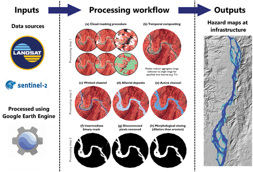
2.1. Satellite imagery analyses

Primary data sources are shown in Table 1; they include Landsat products (30 m spatial resolution; available for 1984-present) and Sentinel collections (10 m spatial resolution; available for 2015-present). Multitemporal, multispectral satellite observations from the Landsat program and Sentinel constellation are particularly useful for disaster resilience applications with archives of data that span almost four decades. We use surface reflectance products from Landsat; the images have been atmospherically corrected, facilitating a more reliable comparison of spectral reflectance measurements between acquisitions. For Sentinel imagery, we use Level 1C products to maximize the record length of imagery.

Table 1. Characteristics of the satellite imagery data used in InfraRivChange.

Data Set	Spatial Resolution	Temporal Revisit	Temporal Archive	Dataset in GEE Catalogue
Landsat 5 TM	30 m	16 days	1984–2012	Landsat 5
Landsat 7 ETM +	30 m	16 days	1999–present	Landsat 7
Landsat 8 OLI/TIRS	30 m	16 days	2013–present	Landsat 8
Sentinel-2 MSI	10 m	10 days	2015–present	Sentinel-2

Abbreviations: ETM-enhanced thematic mapper; MSI-multispectral instrument; OLI-operational land imager; TIRS-thermal infrared sensor; TM-thematic mapper.

A key feature of Landsat and Sentinel data is the availability of multispectral bands, e.g., near-infrared and short-wave infrared. Spectral bands can be combined to calculate multispectral indices, useful for indicating the relative abundance of features of interest such as vegetation and water.

We apply the processing workflow developed by Boothroyd et al. (2021) to classify the active channel from satellite imagery for different time periods and assess shifts in river channel position. The workflow has three main processing steps: (i) cloud masking and temporal compositing; (ii) active river channel classification; and (iii) binary image cleaning. Validation work has been published previously to assess the accuracy of the active river channel classification (Boothroyd et al., 2021). We use similarity coefficients to interpret relative risks of shifting rivers to critical bridge infrastructure based on binary image outputs from the workflow. Differences are identified using the Jaccard index and Dice similarity coefficient. Values closer to 1 indicate greater similarity between active river channel masks, implying that positional shifts in the active river channel were negligible. In addition to similarity coefficients, we also report areal statistics for each of the binary images. We report the number of active channel pixels within the region of interest and the area of the active channel (km²) for each time period of analysis. Changes in the active channel area and similarity coefficients indicate potential threats to critical bridge infrastructure.

2.2. Web application design

We designed a web application (Figure 2) to allow technical and non-technical users to apply the satellite imagery workflow (available online: https://vrindasharma.users.earthengine.app/view/infrariv; and accessible via any web browser, even without a Google account).

Figure 2. Landing page of the InfraRivChange web application.

3. Results

3.1. InfraRivChange demonstration using Landsat imagery

In the first test case we demonstrate results from the Landsat imagery workflow for the Gamu Bridge on the Cagayan River (Figure 3). Using default input parameters, we set the date range as T1 = 01/01/1988 – 01/01/1990 and T2 = 01/01/2018 – 01/01/2020. Results indicate that the section of the Cagayan River has remained approximately stable over the 30-year analysis period. The active channel area has increased marginally (from 2.68 to 2.82 km²), with the Jaccard index (0.81) and Dice similarity coefficient (0.89) indicating a low relative risk to critical bridge infrastructure. Results from InfraRivChange suggest only minor shifts in the active river channel position at this site.

Figure 3. Landsat example from the Gamu Bridge; Cagayan River.

In the second test case we demonstrate results from the Landsat imagery workflow for the Itawes Bridge on the Chico River (Figure 4). Using default input parameters, we set the date range as T1 = 01/01/1988 – 01/01/1990 and T2 = 01/01/2018 – 01/01/2020. Notable here is the mobility of the Chico River in the vicinity of the bridge site over the 30-year analysis period. The active channel area has increased marginally (from 1.41 km² to 1.50 km²), with the Jaccard index (0.53) and Dice similarity coefficient (0.69) indicating a moderate relative risk to critical bridge infrastructure. Results from InfraRivChange suggest moderate shifts in the active river channel position at this site, indicating the need for further investigation and potentially applying more detailed bridge monitoring.

Figure 4. Landsat example from the Itawes Bridge; Chico River.

3.2. InfraRivChange demonstration using Sentinel imagery

In the third test case we demonstrate results from the Sentinel imagery workflow for the Don Mariano Marcos Bridge on the Lagben River (Figure 5). Using default input parameters, we set the date range as T1 = 01/01/2016 – 01/01/2017 and T2 = 01/01/2021 – 01/01/2022. Results indicate that the section of the Lagben River has remained approximately stable over the five-year analysis period. The active channel area has decreased marginally (from 2.12 km² to 1.94 km²), with the Jaccard index (0.83) and Dice similarity coefficient (0.91) indicating a low relative risk to critical bridge infrastructure. Results from InfraRivChange suggest only minor shifts in the active river channel position at this site. However, it is important to note that these changes have occurred over a relatively short timescale (five years, relative to the 30-year timescale of the Landsat workflow).

Figure 5. Sentinel example from the Don Mariano Marcos Bridge; Lagben River.

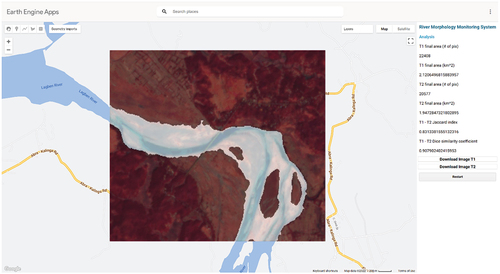
4. Discussion

Satellite imagery analyses offer a low-cost approach for monitoring the relative risk of shifting rivers (> 100 m in width) to critical bridge infrastructure. We propose that satellite imagery analyses can be formally incorporated into bridge monitoring investigations (e.g., as a component of bridge stability assessments) undertaken by primary stakeholders to inform the design and strategic placement of future bridge infrastructure. It has potential for other forms of critical infrastructure adjacent to rivers such as road and rail.

It is important to sense-check outputs from InfraRivChange. Although best efforts have been made to validate and calibrate parameter sets for rivers in the Philippines, all outputs should be sense-checked and critically appraised for other sites. In terms of default values, for Landsat applications we recommend NDVI = 0.2, MNDWI = −0.4 and binary cleaning pixels = 100. For Sentinel applications we recommend NDVI = 0.2, MNDWI = −0.175 and binary cleaning pixels = 300. Individual applications may require customization of default values to improve the classification of the active river channel.

Transferability is used as a term to describe how information or analysis from one region can be applied elsewhere to achieve universality of the approach. The web application can be easily transferred to other dynamic riverine settings where critical bridge infrastructure is at risk from shifting rivers across Southeast Asia. In future, the application may be further developed, validated, calibrated and applied across a geodiverse range of settings. Figure 6 shows an additional example for the Ghaghara River (India) between 1990 and 2020, with the Chahlari Ghat Bridge located at the centre of the image. The Jaccard index (0.15) and Dice similarity coefficient (0.26) are very low, indicating considerable shifts in active channel position. The example demonstrates the potential of transferring the workflow from the Philippines to other dynamic riverine settings.

Figure 6. InfraRivChange web application applied outside of the Philippines, to the Chahlari Ghat Bridge (India).

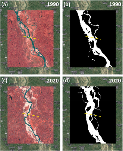
5. Conclusions

We developed a web application to monitor shifting rivers in the vicinity of critical bridge infrastructure in the Philippines. InfraRivChange has been designed to offer non-technical and technical users the opportunity to apply advanced satellite imagery workflows to thousands of Landsat and Sentinel images. The user-friendly web application enables semi-automated multitemporal satellite imagery analyses to be undertaken. Outputs can be used by stakeholders to assess the relative risk of river migration at sites of critical bridge infrastructure. We recommend that InfraRivChange can be used as a low-cost remote sensing approach to monitor shifting rivers at sites of critical bridge infrastructure. Satellite imagery analyses could be formally incorporated into bridge monitoring investigations (e.g., as a component of bridge stability assessments) and inform the design and placement of future infrastructure. We envision that InfraRivChange can be applied to other critical infrastructure adjacent to rivers (e.g., road, rail and pipelines) and extended elsewhere to other dynamic riverine settings.

Acknowledgments

This work was funded by CDRI Fellowship Application no. 201128342. The authors would like to thank the Glasgow University Software Service (GUSS) team, including Tess Vaughan, Tim Storer and Omar Tufayl. We also thank Vrinda Sharma (University of Glasgow) for developing the InfraRivChange web-application through the GUSS initiative. The authors are grateful to Kumar Neeraj Jha (Indian Institute of Technology Delhi) and Kampanart Silva (National Science and Technology Development Agency) for their inputs as Technical Experts during the CDRI Fellowship.

Disclosure statement

The DRI Technical Conference 2022 was sponsored by CDRI, along with editorial work of the Conference Proceedings. However, CDRI did not influence the research, data, findings, and views presented in the research papers.

Mapping landslide susceptibility and critical infrastructure for spatial decision-makingCONTACT Kshitij Dahal [email protected] Dahal [email protected]

ABSTRACT

Landslides pose risks to people, environments and slope infrastructures. Several methodologies have emerged to determine the susceptibility of landslides and their locations. However, susceptibility alone does not provide information about how a landslide will affect infrastructure, making it difficult to understand potential impacts for developing mitigation plans and fortifying vulnerable slopes. The authors propose mapping landslide susceptibility around critical infrastructure, then overlaying and analysing the results to facilitate investment decisions for risk mitigation and resilience. They map multi-temporal landslide susceptibility in Nepal and create an integrated index, then analyse the index with critical infrastructure. This process identifies landslide-prone infrastructures that require investments for mitigation. A web application is developed for easy dissemination of spatial information. They developed the framework in Nepal and found that Province 4 and Province 3 have more landslide-prone infrastructure than other provinces, and thus require mitigation plans and investments. The proposed solution is scalable to other regions to facilitate policy and investment planning to reduce landslide risk.

KEYWORDS:

• landslides
• landslide susceptibility
• critical infrastructure
• infrastructure investment

1. Introduction

Landslides are the most frequent and severe natural hazards in Nepal and the Central Himalayas, causing loss of life and property (Dhakal, 2015). Landslides in the Central Himalayas are characterized by undulating terrain, steep slopes, active seismic faults, earthquake effects, extreme rainfall and anthropogenic factors (Singh et al., 2022). Every year, these landslides do enormous damage during the monsoon, causing damage to infrastructure like roads, towns, health posts, schools and energy (Dahal, 2012).

Several methods have been developed in landslide science, ranging from physically modelling a landslide to statistically modelling a large number of landslides to find likely causes and future locations (Reichenbach et al., 2018). Landslide susceptibility assessment is performed to determine potential landslide areas and vulnerable zones with a likelihood of a landslide being high or low (Shano, Raghuvanshi & Meten, 2020). For large-scale landslide susceptibility modelling, numerous methods based on analytical tools like frequency ratio, analytical hierarchy process, logistic regression and, recently, machine learning models, are being used to support mapping of landslide susceptibility (Park, Heo & Han, 2018).

Although numerous efforts have been made to map landslide susceptibility, success ultimately depends on two factors: first, the data set used to train the model (Wubalem & Meten, 2020), and, second, the environmental conditions and patterns of landslides in that location (Paudyal et al., 2021). Improving the information improves landslide susceptibility models. However, the landslide susceptibility model alone may not provide enough information about the likelihood and impact of landslide disasters (Xiao et al., 2020), because susceptible areas without settlement and infrastructure do not pose a risk to society.

Investment in landslide-prone slopes can help mitigate future landslides and prepare for landslide-resistant infrastructure (Xiao et al., 2020). Infrastructure resilience is its ability, in this case, to recover after a landslide. This necessitates an integration of landslide susceptibility with the presence or absence of infrastructure. Analysing only one typical infrastructure, such as a road, settlement or population (Rusk et al., 2021), does not provide complete information about the presence of critical infrastructure and locations, as other infrastructure can be damaged, resulting in unproductive investments. Emphasis on selective infrastructure, instead of all infrastructure, can lead to poorly informed investment and planning, which will not reduce risk from all aspects and will eventually lead to other losses. This can be mitigated by the integration of all critical infrastructure.

We propose a framework to integrate landslide susceptibility maps, emphasize the dynamic nature of landslide susceptibility, and make a vulnerability assessment of all critical infrastructure. The framework makes it easier to identify locations where investment should be made for the resilience of slope infrastructure at the national level. We also develop a web application to disseminate this information for spatial planning. The application will assist policymakers and practitioners in the efficient assessment of landslide risks to infrastructure and the allocation of investment for reducing these risks.

2. Data and methods

2.1. Landslide inventory

We created a landslide inventory by digitizing the annual base maps of the multi-temporal Planetscope satellite. The Planetscope satellite sensor captures images with a spatial resolution of ~4.7 m. From 2016 to 2020, a multi-temporal landslide was developed at the national level in Nepal.

2.2. Terrain and rainfall derivatives

Terrain derivatives and rainfall derivatives were developed as predictors of landslide susceptibility. Terrain derivatives were created in the Google Earth Engine (GEE) using the Shuttle Radar Topography Mission (SRTM) digital elevation model at 30 m spatial resolution (Safanelli et al., 2020). Rainfall derivatives are derived from the Integrated Multi-satellite Retrievals for GPM (IMERG) and resampled to 30 m spatial resolution. Table 1 and Table 2 present the terrain and rainfall derivatives in detail.

Table 1. Terrain derivatives and definitions used in this study. Modified after (Safanelli et al., 2020).

Name	Description
Elevation	Height of terrain above sea level in metres
Slope	Slope gradient in degrees
Aspect	Compass direction in degrees
Horizontal curvature	Curvature tangent to the contour line in metres
Vertical curvature	Curvature tangent to the slope line in metres
HAND	Height above nearest drainage in metres
TPI	Topographic position Index

Table 2. Rainfall derivatives and definitions used in this study (Talchabhadel et al., 2022).

Symbol	Name	Definitions
CDD	Consecutive dry days	Maximum number of consecutive days with PRCP < 1 mm
CWD	Consecutive wet days	Maximum number of consecutive days with PRCP ≥ 1 mm
PRCPTOT	Annual total wet-day precipitation	Annual total precipitation on wet days (PRCP ≥ 1 mm)
R1	Number of wet days	Annual count of days when PRCP 1 ≥ 1 mm
R10	Number of slightly heavy precipitation days	Annual count of days when PRCP 1 ≥ 10 mm
R20	Number of heavy precipitation days	Annual count of days when PRCP 1 ≥ 20 mm
R50	Number of very heavy precipitation days	Annual count of days when PRCP 1 ≥ 50 mm
r95p	Total annual precipitation from heavy precipitation days	Annual total precipitation in wet days (PRCP ≥ 95 percentile)
r95pTOT	Contribution from heavy precipitation days	Ratio of r95p with PRCPTOT
r99p	Total annual precipitation from very heavy precipitation days	Annual total precipitation on wet days (PRCP ≥ 99 percentile)
r99pTOT	Contribution from very heavy precipitation days	The ratio of r99p with PRCPTOT
R100	Number of extremely heavy precipitation days	Annual count of days when PRCP 1 ≥ 100 mm
RX1day	Max 1-day precipitation	Yearly maximum 1-day precipitation
RX1dayTOT	Contribution from max 1-day precipitation	The ratio of RX1day with PRCPTOT
RX3day	Max consecutive 3-day precipitation	Yearly maximum consecutive 3-day precipitation
RX3dayTOT	Contribution from max 3-day precipitation	The ratio of RX3day with PRCPTOT
RX5day	Max consecutive 5-day precipitation	Yearly maximum consecutive 5-day precipitation
RX5dayTOT	Contribution from max 5-day precipitation	The ratio of RX5day with PRCPTOT
RX7day	Max consecutive 7-day precipitation	Yearly maximum consecutive 7-day precipitation
RX7dayTOT	Contribution from max 7-day precipitation	The ratio of RX7day with PRCPTOT
SDII	Simple daily intensity index	Average precipitation on wet days (PRCPTOT/R1)

2.3. Landslide intensity susceptibility index (LISI)

Landslide susceptibility mapping was performed in GEE using landslide inventory as a target variable and terrain and rainfall derivatives as independent variables. We used the GEE’s random forest classifier to generate a landslide susceptibility map in the form of a probabilistic index (0–100) for the years 2016 to 2020.

The validation of landslide susceptibility maps was done statistically using the area under the receiver characteristic curve (AUC-ROC) method. The AUC-ROC method has been used by many researchers (Mehrabi, 2022; Pham et al., 2016; Sarkar & Kanungo, 2004) and is a reliable method to validate susceptibility models (Vakhshoori & Zare, 2018).

The landslide intensity susceptibility index (LISI) is then calculated using five different susceptibility maps, and each pixel is assigned a value between 1–10 based on the presence of a landslide susceptible zone on that specific pixel over five years.

2.4. Critical infrastructure spatial index (CISI)

We created CISI using OpenStreetMap (https://www.openstreetmap.org). An OpenStreetMap dataset was compiled to create a raster image with values ranging from 0–10 based on the presence of critical infrastructure. For example, a value of 10 indicates that all seven types of critical infrastructure are present in that particular pixel, whereas a value of 0 indicates no critical infrastructure.

2.5. Landslide Management Information System (LMIS): web application

We developed a web application named LMIS (Landslide Management Information System) based on the GEE to provide LISI and CISI spatial maps, allowing for spatial planning (Figure 1).

Figure 1. Overall methodology to map LISI, CISI and the web application.

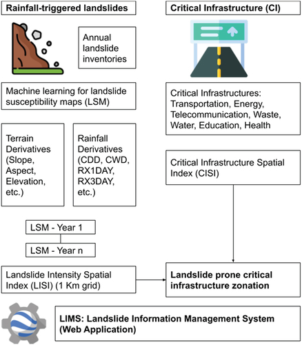
3. Results and discussion

3.1. Landslide susceptibility and validation

Figure 2 depicts a landslide susceptibility map created over a five-year period. Green indicates less/safe landslide susceptibility, whereas red indicates greater landslide susceptibility in the region. A constant/consistent higher susceptibility is observed in the central part of Nepal, with two pockets observed in the eastern and western parts of the country. The western part is inconsistent and varies, primarily due to varying patterns of rainfall in these regions. Such inconsistencies also indicate the greater possibility of future climate change impacts in these areas, as susceptibility is primarily controlled by extreme rainfall. It is worth noting that landslide susceptibility is a dynamic and time-dependent phenomenon based on extreme rainfall variations.

Figure 2. Annual landslide susceptibility map for years 2016 to 2020 produced using a random forest model in Google Earth Engine.

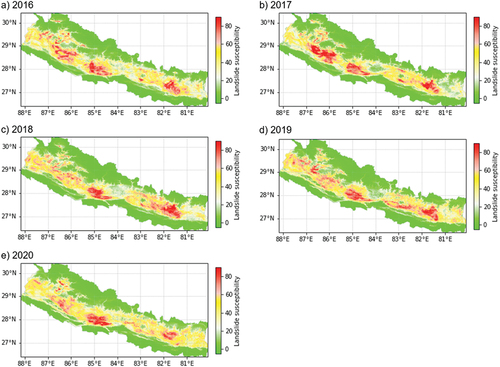
The landslide susceptibility models require validation before trusting the models, and AUC-ROC and OBG errors are presented in Table 3. The scores obtained in both metrics are reliable and align to the recent studies about landslide susceptibility validation (Chen & Chen, 2021; Mehrabi, 2022). In AUC-ROC validation, all five models performed similarly, indicating that the results are comparable and reliable.

Table 3. Validation score of landslide susceptibility maps: (i) area under the curve value (higher is better); and (ii) out of bag error in random forest model training (lower is better).

Year	Area Under the ROC Curve Score	Optimized Out of Bag Error
2016	0.94	0.13
2017	0.94	0.12
2018	0.94	0.12
2019	0.93	0.13
2020	0.93	0.13

3.2. LISI, CISI and overlay analysis

Figure 3 depicts LISI, CISI and scenarios in which both indices exceed the threshold. Figure 3 a depicts a five-year integrated landslide susceptibility assessment classified into 10 different classes, where the green colouring implies landslides are extremely rare in that particular area, and the rate indicates that it has been found to be sensitive consistently over five years. Figure 3(b) depicts the presence and absence of critical infrastructure, which are also ranked from 0 to 10 across 10 different classes. The value 0 represents the absence of all infrastructure, while the value 10 represents the presence of all seven critical infrastructures. The LISI and CISI are created with a spatial resolution of 1 km. Figure 3(c) depicts areas where both CISI and LISI are greater than 5, implying that these are the critical infrastructure locations located in landslide prone areas.

Figure 3. (a) LISI map classes; (b) CISI map classes; and (c) LISI overlaid on CISI classes (LISI > 5 and CISI > 5).

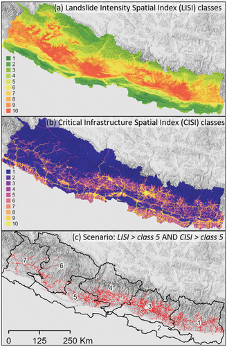
The critical infrastructures of Province 4 and Province 3 were found to be in landslide-prone areas, necessitating property investment and mitigation plans, followed by Province 1. Province 2 is considered a relatively safe zone due to its lower elevation and less susceptible zone. Provinces 5, 6 and 7 appear to be susceptible to river corridors; these river corridors are also important connectors for highways and settlements, and they are prone to landslides. Based on these observations, investment plans and planning for new infrastructure can be developed.

3.3. Web application

A web application based on Google Earth Engine has been developed to aid in the provision of spatial data for policymakers and investment planners (Figure 4). The application also allows multiple maps to display their legend information and Nepal’s administrative layer to filter and make decisions. The web app can be accessed here: https://geokshitij.users.earthengine.app/view/lims

Figure 4. Snapshot of a web application for dissemination of LISI, CISI and other relevant datasets. The snapshot shows LISI of Nepal.

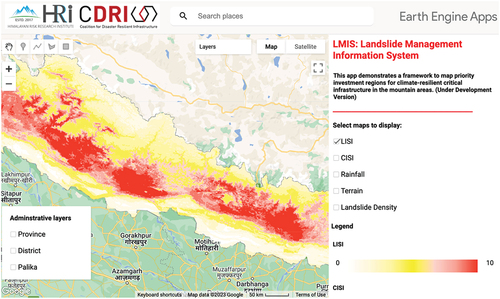
4. Conclusion

This study proposes a methodology for identifying landslide-prone critical infrastructure to support risk-informed investment decisions. First, we proposed the mapping of multi-temporal landslides and developing a landslide intensity susceptibility index. Second, we created a critical infrastructure index in OpenStreetMaps by combining different layers, and we discovered critical infrastructure in landslide-prone areas by overlay analysis with landslide susceptibility. This identifies landslide-prone critical infrastructure that requires mitigation and provides an assessment of the infrastructure’s resilience. We also created a web application using the Google Earth Engine to share spatial information about landslide susceptibility and critical infrastructure in Nepal. This framework is scalable and can be used for other regions to identify critical infrastructure that is vulnerable to landslides. Full paper published in the Science of The Total Environment (Gnyawali et al., 2023) on 15 February 2023.

Acknowledgments

The authors would like to thank Dr Rocky Talchabhadel (Texas A&M University) for providing rainfall indices data and Dr Sadhana Nirandjan (TU Delft) for providing CISI of Nepal. We also acknowledge the suggestions from Dr Ranit Chaterjee (Kyoto University) at various stages of this research. This research is funded by the 2021–2022 Fellowship of the Coalition for Disaster Resilient Infrastructure (CDRI), Application ID: 210113422.

Disclosure statement

The DRI Technical Conference 2022 was sponsored by CDRI, along with editorial work of the Conference Proceedings. However, CDRI did not influence the research, data, findings, and views presented in the research papers.

Comprehending school disaster resilience: deriving indicators for risk-informed school evaluation

ABSTRACT

Disasters or extreme events in schools and on their peripheries damage a school’s infrastructure, result in injuries to students and staff or create temporary closure, disrupting continuity of education. Disaster risks are rarely considered while selecting schools. School selection is driven by academic achievement, curriculum and the quality of the teachers in the school, with less or no focus on school disaster resilience aspects. This paper attempts to identify indicators for evaluating schools based on two important factors: parental school selection and school disaster resilience. The research methodology adopts a literature review and a three-phase Delphi method. A total of 22 experts from three groups – disaster management, academicians and parent–teacher association members – participated in the survey. The paper summarizes final indicators that the authors used for developing the Risk Informed School Evaluation (RISE) tool as part of their study under the 2021–2022 CDRI Fellowship Programme of the Coalition for Disaster Resilient Infrastructure (CDRI). The study recognizes the significant themes that are pivotal in parental school selection, and that school disaster resilience can systematically aid school management in capacity-building and preparedness for disaster risks.

KEYWORDS:

• Disaster resilience
• school safety
• school evaluation
• critical infrastructure

1. Introduction

Schools are an essential part of society’s infrastructure and serve as the secondary residence for children between the ages of 3 to 18 (NIDM, 2018), making a school’s security of paramount concern. The geographical locations of schools are decided without considering risks from surrounding hazards (NDMA, 2016). Risks are further complicated by limited knowledge about changes in hazards and land use, which endangers lives. The world has witnessed many school-related accidents/disaster events. Pazzi et al. (2016) listed over 31 of the worst geo-hydrologic events between 2004 and 2015 across the globe having direct impact on schools and schoolchildren in terms of victims, injuries and psychological consequences when assessing the safety of schools affected by geo-hydrologic hazards.

In India alone, several disasters directly affected schools and children, such as the 2004 Indian Ocean Tsunami, the 2004 Kumbakonam Fire Tragedy in Tamil Nadu, the 2001 Gujarat Earthquake and the 1995 Dabwali Fire Accident in Haryana. More recently disasters such as a fire at a coaching centre in Surat (Gujarat) and the Pune Floods in 2019 highlight the need to focus on school safety along with school curricula. The national school safety programme in India and similar efforts on school safety in Japan have focused on overall school safety, but there is a dearth of decision-making tools concerning school infrastructure and associated risk patterns (Nakum et al., 2022).

For a country like India, additional factors complicate problems. India is vulnerable to various hazards because of geographical locations, topography and anthropogenic reasons. The National Disaster Management Authority of India states that around 59% of the Indian landmass is at risk of moderate to extreme earthquakes, and 12% is prone to flooding and soil erosion. Similarly, the region is vulnerable to various other natural and man-made disasters. Such vulnerability is highly significant as India has the highest student population in the world and has a history of student casualties during disasters such as the Gujarat Earthquake in 2001 and the Kashmir Earthquake in 2005 (UN-ESCAP, 2019).

2. Research problem

Several policies have evolved to address the existing and emerging disaster risks, such as the National Disaster Management Act (2005), the National Policy of Disaster Management (2009) and the National School Safety Policy of India (2016). However, the recent cyclone Fani (2019) resulted in damage to over 6500 schools in the state of Odisha (Times of India, 2019), reiterating the importance of improved research and learning for school resilience. Further, limited efforts at capacity-building combining school academics and school resilience adds to the issue (Nakum et al., 2022).

Even though clause 19 of India’s Right to Education Act (2009) forbids/prohibits the construction of school buildings in disaster-prone zones, various instances such as the 2019 Pune floods show otherwise. The school safety policy (2016) recommends improving internal and external factors of school safety for effective disaster response. This is further supported by the National Education Policy (2020) which advocates the inclusion of disaster response and first aid in school curricula. While policy support is ensured, ground implementation remains a challenge. Further, the monitoring of risk mitigation and reduction interventions remain privy to the government and school administration while parents and students remain mostly uninformed. To address incumbent gaps in school selection and resilience, as discussed earlier, this study aims to delve into the following questions:

1. What are the pivotal factors considered by parents when choosing a school for their children?

2. What are the critical factors for school safety and resilience?

3. Objective

The objective of the study was to identify the relevant themes and indicators for parental school selection and school disaster resilience using the case study of Gandhinagar, India.

4. Methodology

The paper expands the ongoing research by the authors under the 2021–2022 CDRI Fellowship Programme on the Risk Informed School Evaluation (RISE) tool. Using an integrative literature review method, the authors listed 69 indicators that affect parental school selection and school disaster resilience (Nakum et al., 2022). This study further used the Delphi technique/method to gain consensus over indicators through three phases of questionnaires (Figure 1).

Figure 1. Methodology of the study.

The Delphi method is used to gain consensus through phases of questionnaires, usually two or three, where information and results are fed back to panel members between each phase (Loo, 2002; Yao & Liu, 2006). The survey questionnaire and results were shared with experts between phases. A total of 22 experts from three distinct groups – disaster management experts, academicians and parent–teacher association members – participated in the survey.

5. Analysis and results

To finalize the indicators identified through the literature review, a three-phase Delphi process was carried out. The experts were asked to give their opinions in a Google survey form. If the experts deemed certain indicators or themes to be irrelevant, they could advise their elimination. Analysis of phase I shortlisted 54 indicators out of 69 to be important, including 21 indicators for school disaster resilience and 33 indicators for parental school choice. Experts also suggested additional factors such as the faculty retention rate, the affordability of transport services, the student attendance rate, the availability of scholarships, the frequency of parent–teacher meetings (PTM) and the proximity to highways or main roads with traffic.

The finalized themes and 54 indicators of phase I were subjected to further consensus. The indicators were subjected to Likert Scale 1–5 rating with 1 being least important and 5 being highly important. The Delphi results were based on two preconditions. One is a strong agreement between experts, which is indicated by values ≥4 and was set at 51% or above. The second was the standard deviation (S.D.) that was set at <1.5 (Christie & Barela, 2005; Giannarou & Zervas, 2014). The results showed that from 54 indicators, 43 attained consensus (Table 1) and 11 attained non-consensus (Table 2). Among the 43 consensus indicators, 30 (out of 33 indicators) belonged to parental school selection and 13 (out of 21) indicators belonged to school disaster resilience.

Table 1. Result of Delphi survey phase II: consensus indicators.

Sr. No.	Indicators	Agreement %	S.D.
	Parental school selection indicators
1	Passing percentage of students in board examinations	91.6	0.51
2	Percentage of students with top scores/high performing students in board/final examinations	75	0.68
3	School’s academic achievements at state/national/international level competition	83.3	0.71
4	Number of teaching staff available with respect to number of children	100	0.52
5	Availability of experienced staff in the school	91.6	0.65
6	Availability of teachers with specialization	91.6	0.65
7	Faculty retention rate of the school	91.6	0.65
8	Availability of public/private transport	91.66	0.67
9	Safety of transport facilities	83.3	0.77
10	Affordability of transport services	83.3	0.75
11	Availability of a clean school environment (free from pollution, waste-free environment, etc.)	75	0.95
12	Availability of subject specific laboratory facilities	83.33	0.75
13	Availability of smart classrooms	58.33	1.1
14	Availability of recreational facilities (playgrounds, gyms)	66.6	1.11
15	Availability of basic amenities such as safe drinking water and sanitation	100	0.51
16	Availability of disciplinary policies in the school	75	0.83
17	Presence of student cell/counsellor for student related issues	66.6	1.11
18	Inclusivity of the school in terms of caste, gender and religion	75	1.26
19	Presence of inclusive designs to accommodate the physically challenged/disability friendly campus	58.3	1.49
20	Safety of external surrounding (crime-free neighbourhoods)	83.33	0.75
21	Student attendance rate	75	1.02
22	Frequency of parent–teacher meetings (PTM)	58.33	1.18
23	Regular updates on student progress, school programmes and policy revisions	83.33	0.71
24	Regular check on parents’ feedback and action as per recommendations	75	0.95
25	Public opinion on the school	75	0.66
26	The curriculum/syllabus of the school (CBSE/ICSE/state board)	85	0.75
27	Medium of communication	85	0.71
28	Cost/fee of the school	71	0.89
29	Presence of co-curricular activities such as academic conferences	71	1.15
30	Presence of extra-curricular activities such as sports	57	1.49
	School disaster resilience indicators
31	Building is built as per prevailing norms such as building codes, municipal bylaws, fire safety regulations, SSA and school safety guidelines.	66.6	1.33
32	Schools undergo regular structural safety checks and maintenance	58.33	0.99
33	Designed and demarcated emergency evacuation routes in the building	83.33	0.71
34	Fool proofing of non-structural elements (such as false ceiling, obstruction-free staircases, measures are taken in libraries, laboratories, offices)	75	0.99
35	School has updated School Disaster Management Plan (SDMP)	75	1.02
36	Teachers and staff are regularly trained on disaster risk management	66.66	0.99
37	School has dedicated emergency resources such as fire hydrants, first aid kits, emergency funds, fire alarms for early warning and response.	58.33	0.98
38	Schools have demarcated assembly points during emergencies	58.33	0.9
39	Proximity to highways or main roads with high traffic	66.6	0.8
40	Availability of internet security and secure use of services in school network	75	1.12
41	Student and staff awareness on safe use of social networking sites to check cyber-crimes	66.66	1.37
42	Promoting awareness of parents on IT security and child lock system	66.6	1.24
43	Presence of school cyber/internet policy and protocols	58.33	1.48

Table 2. Result of Delphi survey phase II: non-consensus indicators.

Sr. No.	Indicators	Agreement %	S.D
1	School undertakes regular mock exercises on disaster risk management (DRM)	50	1.30
2	School has integrated disaster risk management in school curriculum	50	1.38
3	Availability of insurance and emergency funds for the schools	50	1.441
4	Frequency of hazards in the region	50	1.44
5	Severity of hazards in the region	50	1.38
6	Presence of hazardous industries/unsafe conditions in the region	50	1.31
7	School management have active interaction with local authorities, emergency response agencies, and communities nearby for disaster responses	41.66	1.3
8	Availability of scholarships	50	1.6
9	Influence from friends and relatives	50	0.86
10	Age of the building structure	50	1.14
11	Distance from the school	50	1.08

Table 3. Result of Delphi survey phase III.

Sr. No.	Indicators	Agreement %	S.D.
	Consensus indicators
1	School management have active interaction with local authorities, emergency response agencies and communities nearby for disaster responses	75	1.08
2	School has integrated disaster risk management in school curriculum	66.66	1.38
3	Presence of hazardous industries/unsafe conditions in the region	66.6	1.41
4	Influence from friends and relatives	58.33	0.69
5	Availability of insurance and emergency funds for the schools	58.11	1.29
6	Frequency of hazards in the region	58.11	1.21
	Non-consensus indicators
1	School undertakes regular mock exercises on disaster risk management (DRM)	50	1.30
2	Severity of hazards in the region	50	1.38
3	Distance from the school	50	1.12
4	Availability of scholarships	41.66	1.3
5	Age of the building structure	41.66	1.29

Table 1. Result of Delphi survey phase II: consensus indicators.

Sr. No.	Indicators	Agreement %	S.D.
	Parental school selection indicators
1	Passing percentage of students in board examinations	91.6	0.51
2	Percentage of students with top scores/high performing students in board/final examinations	75	0.68
3	School’s academic achievements at state/national/international level competition	83.3	0.71
4	Number of teaching staff available with respect to number of children	100	0.52
5	Availability of experienced staff in the school	91.6	0.65
6	Availability of teachers with specialization	91.6	0.65
7	Faculty retention rate of the school	91.6	0.65
8	Availability of public/private transport	91.66	0.67
9	Safety of transport facilities	83.3	0.77
10	Affordability of transport services	83.3	0.75
11	Availability of a clean school environment (free from pollution, waste-free environment, etc.)	75	0.95
12	Availability of subject specific laboratory facilities	83.33	0.75
13	Availability of smart classrooms	58.33	1.1
14	Availability of recreational facilities (playgrounds, gyms)	66.6	1.11
15	Availability of basic amenities such as safe drinking water and sanitation	100	0.51
16	Availability of disciplinary policies in the school	75	0.83
17	Presence of student cell/counsellor for student related issues	66.6	1.11
18	Inclusivity of the school in terms of caste, gender and religion	75	1.26
19	Presence of inclusive designs to accommodate the physically challenged/disability friendly campus	58.3	1.49
20	Safety of external surrounding (crime-free neighbourhoods)	83.33	0.75
21	Student attendance rate	75	1.02
22	Frequency of parent–teacher meetings (PTM)	58.33	1.18
23	Regular updates on student progress, school programmes and policy revisions	83.33	0.71
24	Regular check on parents’ feedback and action as per recommendations	75	0.95
25	Public opinion on the school	75	0.66
26	The curriculum/syllabus of the school (CBSE/ICSE/state board)	85	0.75
27	Medium of communication	85	0.71
28	Cost/fee of the school	71	0.89
29	Presence of co-curricular activities such as academic conferences	71	1.15
30	Presence of extra-curricular activities such as sports	57	1.49
	School disaster resilience indicators
31	Building is built as per prevailing norms such as building codes, municipal bylaws, fire safety regulations, SSA and school safety guidelines.	66.6	1.33
32	Schools undergo regular structural safety checks and maintenance	58.33	0.99
33	Designed and demarcated emergency evacuation routes in the building	83.33	0.71
34	Fool proofing of non-structural elements (such as false ceiling, obstruction-free staircases, measures are taken in libraries, laboratories, offices)	75	0.99
35	School has updated School Disaster Management Plan (SDMP)	75	1.02
36	Teachers and staff are regularly trained on disaster risk management	66.66	0.99
37	School has dedicated emergency resources such as fire hydrants, first aid kits, emergency funds, fire alarms for early warning and response.	58.33	0.98
38	Schools have demarcated assembly points during emergencies	58.33	0.9
39	Proximity to highways or main roads with high traffic	66.6	0.8
40	Availability of internet security and secure use of services in school network	75	1.12
41	Student and staff awareness on safe use of social networking sites to check cyber-crimes	66.66	1.37
42	Promoting awareness of parents on IT security and child lock system	66.6	1.24
43	Presence of school cyber/internet policy and protocols	58.33	1.48

Table 2. Result of Delphi survey phase II: non-consensus indicators.

Sr. No.	Indicators	Agreement %	S.D
1	School undertakes regular mock exercises on disaster risk management (DRM)	50	1.30
2	School has integrated disaster risk management in school curriculum	50	1.38
3	Availability of insurance and emergency funds for the schools	50	1.441
4	Frequency of hazards in the region	50	1.44
5	Severity of hazards in the region	50	1.38
6	Presence of hazardous industries/unsafe conditions in the region	50	1.31
7	School management have active interaction with local authorities, emergency response agencies, and communities nearby for disaster responses	41.66	1.3
8	Availability of scholarships	50	1.6
9	Influence from friends and relatives	50	0.86
10	Age of the building structure	50	1.14
11	Distance from the school	50	1.08

The third phase resulted in more indicators moving from non-consensus to consensus as given in Table 3, such as frequency of hazards, emergency funding, interactions with local agencies and so on. However, certain aspects that are critical to disaster resilience such as the age of the building, the intensity of hazards and the conduct of mock exercises did not receive consensus, which may indicate lower awareness amongst the stakeholders concerning school safety.

Table 3. Result of Delphi survey phase III.

Sr. No.	Indicators	Agreement %	S.D.
	Consensus indicators
1	School management have active interaction with local authorities, emergency response agencies and communities nearby for disaster responses	75	1.08
2	School has integrated disaster risk management in school curriculum	66.66	1.38
3	Presence of hazardous industries/unsafe conditions in the region	66.6	1.41
4	Influence from friends and relatives	58.33	0.69
5	Availability of insurance and emergency funds for the schools	58.11	1.29
6	Frequency of hazards in the region	58.11	1.21
	Non-consensus indicators
1	School undertakes regular mock exercises on disaster risk management (DRM)	50	1.30
2	Severity of hazards in the region	50	1.38
3	Distance from the school	50	1.12
4	Availability of scholarships	41.66	1.3
5	Age of the building structure	41.66	1.29

6. Conclusion

The analysis gives key insights concerning school safety amongst stakeholders. For example, in phase II, 90% of parental school selection indicators received consensus, while only 60% of the school disaster resilience indicators received consensus. Several indicators concerning the presence of hazards did not receive consensus. This indicates the bias of stakeholders towards school academic progress reports rather than disaster resilience aspects. However, the findings demonstrate a strong consensus on indicators identified as part of the study, which can serve as entry points for enhancing school safety.

School infrastructures are a major part of nation-building. Schools also serve as safe shelters or evacuation points during disasters, hence they must be physically safe. Under the National School Safety programme in India, schools are encouraged to prepare disaster management plans and with a rapid assessment. So, these indicators can serve a two-pronged benefit of aiding parents in school selection and ensuring a school’s administration of school preparedness for any eventuality.

Acknowledgments

This study is part of the 2021–2022 CDRI Fellowship Programme (Application ID: 210,117,475) awarded by the Coalition for Disaster Resilient Infrastructure.

Disclosure statement

The DRI Technical Conference 2022 was sponsored by CDRI, along with editorial work of the Conference Proceedings. However, CDRI did not influence the research, data, findings, and views presented in the research papers.

Empowering decision-makers to take resilient action towards urban heat island mitigation by developing a multi-dimensional climate modelCONTACT Parisa Kloss [email protected]; [email protected]

https://www.linkedin.com/in/parisa-kloss-93b61930/; https://www.linkedin.com/in/mojtaba-samimi-06178840/

ABSTRACT

A barrier to resilient action on climate issues such as urban heat island (UHI) effect is the lack of appropriate technological tools to visualize existing hotspots for mitigation planning. Many tools support measurement of UHI effect like remote sensing, mobile traverses, historical weather data and others. But analyses and results of these tools are not visually intuitive for stakeholders. Although higher temperatures in an urban area can be proven with scientific measurements, how to accurately recognize the responsible elements remains unclear. Emerging technology can facilitate development of models that can support previous methodologies, investigate the issue from various dimensions and empower decision-makers to take long-lasting resilient action within time and budget. To overcome the existing barrier, a multi-dimensional climate model, using a computational platform called ‘Solarchvision’, has been developed to optimize climatic performance of cities from various dimensions. It adopts a spatial analysis to identify hotspots, analyse them and develop potential and optimum corrective measures. The model can also serve as a basis for granting construction permits, enabling cities to take accelerated and more ambitious climate action, as well as achieve related sustainable development goals (SDGs) on the ground. The model has been tested in a pilot case study in Montreal, Canada.

Keywords:

• urban heat island effect
• climate action
• multi-dimensional climate model
• climate resilient cities

1. Introduction

Development planning with little attention to local climate and extreme weather causes long-term adverse effects on the environment. Increasing ambient temperature can put citizens at great risk for morbidity and mortality. In addition, indoor and outdoor thermal discomfort are common problems in many cities. Incorrect location, orientation and design of multi-storey and high-rise buildings create microclimate changes in urban areas known as the urban heat island (UHI) phenomenon.

It is crucial to mitigate UHI effect and optimize for urban thermal comfort in cities. Taking best actions towards tackling UHI necessitates access to reliable data and tools while following up-to-date methods and guidelines. In this regard, potential valuable data must be identified, collected and processed to enable smart/effective decision-making processes and sustainable designs.

This paper introduces a multi-dimensional climate model through a case study in Montreal, Canada. To optimize the climatic performance of the city, applying a spatial analysis, which helps identify the hotspots, study and develop potential corrections and then evaluate optimum solutions, is essential. This approach aims to empower decision-makers with more effective sustainable designs and action plans.

1.1. The UHI phenomenon and challenges in cities

The majority of cities around the world are struggling with UHI effects, such as severe and frequent heat waves associated with global climate change. UHI occurs when an evaporation deficit in the city is created by replacing natural environments with sealed urban areas. Hence, the solar radiation absorbed by urban materials such as asphalt, concrete and stone during the day emit to the ambient air at night, creating high temperature differences between urban and rural areas (Emmanuel, 2005; Landsberg, 1981; Oke, 1987; Shahmohamadi (Kloss) et al., 2011).

The intensity of UHI and its occurrence time depends on the unique characteristics of a city such as location, population size, density of built-up areas, urban geometry and construction materials (Givoni, 1998). Moreover, air pollution, anthropogenic heat, meteorological parameters and residents’ activities also exacerbate UHI effect (Ludwig, 1970). Human and economic activities, which may include space cooling and heating, lighting, manufacturing and traffic congestion (or vehicles), are responsible for a high percentage of anthropogenic heat release. UHI effect increases demand for air conditioning, which in turn causes higher local and regional air pollution through power generation from fossil fuels.

Different approaches to measuring UHI are: (i) fixed stations; (ii) mobile traverses; (iii) remote sensing; (iv) vertical sensing; and (v) energy balance (Gartland, 2008). But each of them has its own limitations. For instance, remote sensing is useful for identifying hotspots on horizontal surfaces like roofs, pavements, vegetation and bare ground. It leaves out the temperature of vertical surfaces like walls, as well as the temperature under trees. These vertical and shaded surfaces are just as important to UHI as the surface seen from above.

Today’s emerging technology equips us to develop models that can fulfil the gaps in previous approaches and methodologies, investigate the issue from various dimensions in a complex system, and give us a broad view to solve the problem and make smart/effective decisions.

1.2. Mapping land surface temperature (LST) in Montreal

By mapping LST, plenty of summer hotspots were identified over the island of Montreal. Google Earth Engine Open-Source Code for LST estimation from the Landsat Series-Remote Sensing (Ermida et al., 2020) has been applied to map LST. The satellite image was derived from Landsat 8. Since the warmest days of Montreal are in July, LST has been mapped for the date range of 1–15 July 2020.

Figure 1 shows several hotspots on the island of Montreal, with surface temperatures between 42°C and 47°C, especially in the western and eastern parts with industries and limited greenery. These areas are covered with large-scale low albedo materials, which are more exposed to the sun and absorb higher solar radiation during the day. On this map, greeneries are the coolest areas, with temperatures between 17°C and 27°C, because of their lower heat capacity, which absorbs and retains less solar radiation. The surface temperatures of downtown Montreal are also high in some parts where the greenery is less. Notably roofs, parking lots and bare land are among the hottest surfaces in the downtown.

Figure 1. Montreal and the Place Bonaventure case study area LST maps.

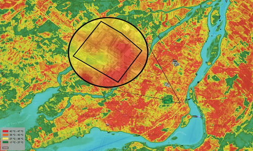
After selecting a high-risk urban area based on the LST map, visualization of hotspots in three dimensions should be performed to discover the impacts of certain climatic parameters, namely air temperature and solar radiation, on landscape and architectural elements in the urban environment over time.

This study has chosen Place Bonaventure as a hotspot in downtown Montreal to run the spatial model analysing how buildings’ arrangements, their forms, orientation and materials contribute to intensification of UHI effect. The model also helps to visualize and prioritize high-risk spots from different dimensions, for instance, 3-D, time and scenarios.

2. Multi-dimensional climate model

A multi-dimensional climate model was performed through a computational platform called Solarchvision. The model is based on the 3-D model of buildings, shading devices, trees and topography. The fourth and fifth dimensions are shaped along climatic and weather data of the location across different hours and seasons.

2.1. Solar radiation

Figure 2 shows plots of hourly ‘direct beam radiation’ on each day during different months for Montreal in 2020. The diagram represents that the low altitude of the sun after sunrise and before sunset can decrease the amount of direct beam radiation significantly. On the other hand, around noon, direct beam radiation reaches its maximum point in May, June, July and August, and on sunny days in winter, and could reach high values of over 1000 W/m² for several hours. A remarkable observation is on sunny days, where the amount of direct radiation is high, and the probability of having an extreme high temperature during summer and extreme low temperature during winter is also high. In fact, the coldest days during the winter and hottest days in summer are the sunny days.

Figure 2. Hourly direct beam radiation of Montreal for two half-cycles of 2020.

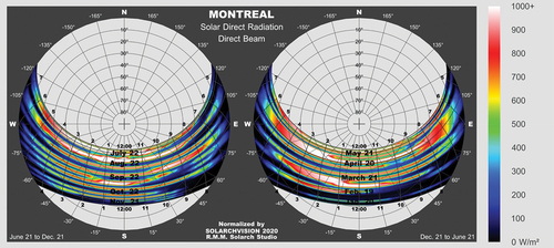
2.2. Temperature pattern

Figure 3 shows the hourly temperature for Montreal in 2020. It presents a current pattern of temperature, including extremes in which air temperature reached +36°C on 27 May and -24°C on 9 February. As a result, Montreal is struggling with extreme weather events during both winter and summer periods.

Figure 3. Hourly air temperature from sunrise to sunset in Montreal in 2020.

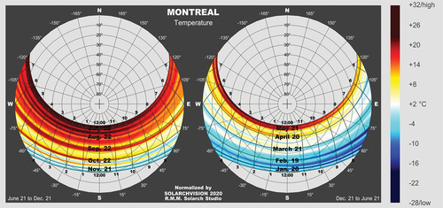
2.3. Positive and negative effects of the sun

The positive and negative effects of the sun depend on the amount of solar radiation and the difference between outdoor temperature and desired indoor temperature as defined by the Degree of Need to Shade/Shine (Samimi, 2007). By multiplying the hourly amount of the direct solar beam radiation with the degree of Need to Shade/Shine in each hour during different months of the year, the positive and negative effects of the direct beam radiation can be calculated (Figure 5). This parameter can help to identify extreme times and scenarios.

Figure 4 shows the positive and negative effects of direct solar radiation in relation to cold/warm weather during half an annual cycle for Montreal. The most undesirable effects of the sun occur when both air temperature and solar radiation are high. As plotted in red, the most undesirable effects usually occur between 6 am and 6 pm from May to August. The negative effect of the sun in summer is not immediately after sunrise or in the last hours before sunset, as the amount of direct radiation decreases significantly when the altitude of the sun is 15° or lower.

Figure 4. Hourly positive/negative effects of direct solar radiation in Montreal in 2020.

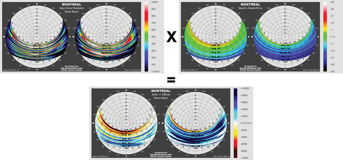
The results also highlight time and position of the sun for which its positive impact is greatest. When the altitude of the sun is 15° or lower, the amount of direct radiation decreases significantly, as the rays pass extra distance across layers of the atmosphere. Therefore, despite low temperatures, which generally occur at the time of sunrise, positive effects of the sun reach their maximum a few hours after sunrise, when the sun is at a higher altitude and air temperature is still low.

To have a better view of the likely and extreme scenarios in future as well as their impact levels, the past climatic condition should also be analysed in detail. Figure 5 and Figure 6 show distributions and probabilities of active and passive urban solar impacts in different months in Montreal from 1953 to 2005. The figures show that during these 53 years, the solar potentials/impacts are likely to be greater in July. In addition, Figure 7 presents the extreme temperature scenario during these years, which occurred not only in June and July, but also from April to September. These analyses help with comprehensive perception of the past scenarios and better predictions about future scenarios.

Figure 5. Extreme negative solar impacts in relation to high air temperature scenarios in Montreal across different months based on 1953–2005 data.

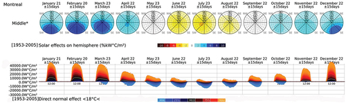
Figure 6. Distribution, probabilities and passive solar impacts in Montreal across different months using 1953–2005 data.

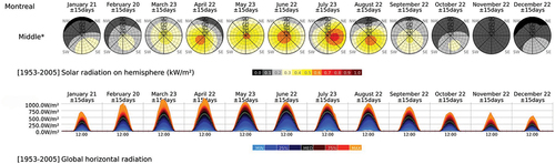
Figure 7. Distributions, probabilities and active solar potentials in Montreal across different months using 1953–2005 data.

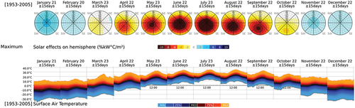
2.4. Spatial climatic analysis in design

Spatial analysis can be applied throughout the design process, covering basic models as well as detailed and complex ones. This analysis improves design for a better quality of indoor and outdoor spaces, as well as a meaningful integrated design of the built environment (Samimi & Nasrollahi, 2014). For instance, these analyses help us to find the best position for windows and skylights to improve the energy performance of the buildings’ envelopes.

2.5. Effects on urban fabric and building skin

The thermal characteristics of an urban fabric can contribute to intensifying UHI effect. Urban materials absorb and retain solar radiation, which increase the heat capacity of the urban fabric. Further, due to the complex urban geometry, reflections of longwave solar radiations multiply and get trapped in the urban canyons. This causes a reduction in air ventilation and restricts the cosmic cooling effects at night.

Figure 8 mapped this analysis in the existing urban fabric of the case study area, for 90 days from 1 June to 2 September 2020. Red spots show high risk areas or the most negative performances, and blue indicates the most positive climatic design performances. Negative impacts that building geometries have on each other, as well as that on the urban area, are plotted in red (Figures 9 and 10). The figures show that roofs and buildings oriented to southeast and southwest, as well as the paths in East–West directions, should be the first priorities for action. Shading devices are needed in some building facades oriented northeast and northwest to improve the climatic performances from yellow to blue.

Figure 8. The positive and negative effects in urban context Montreal, June–September 2020

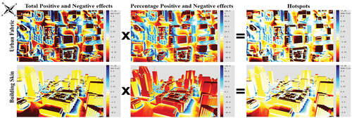
Figure 9. The hotspots in Place Bonaventure’s urban fabric.

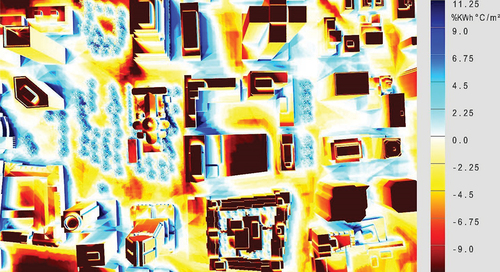
Figure 10. The hotspots in Place Bonaventure’s building skins.

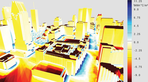
Building skins define the border between indoor and outdoor and they play a crucial role in adjusting the energy demand of a building. Material, shape and orientation of different surfaces, ranging from the roof to the façades of a building, determine the quality of indoor air. The skin should be designed to benefit from external positive conditions, as well as to protect from undesirable effects of natural and built environments.

2.6. Analysing scenarios

After identifying the hotspots and prioritizing them, different scenarios are developed and simulated to find out which of them could have a positive impact on the hotspots. Based on these simulations, and by ranking different design choices for their long-term effects, actions could be prioritized. A mitigation plan to mitigate UHI effect in the target area can be developed.

Figure 11 shows a simulated scenario. By placing trees on a hotspot, the surface temperature of that area dropped up to 5°C. Trees produce desirable shading effects during summer to improve the climatic performance of a place, as well as provide thermal comfort for people and protect them from undesirable solar radiation. They can also revitalize an area for walking and gathering.

Figure 11. Scenario simulation with and without trees.

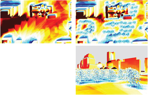
3.0. Conclusion

Today, modern technology makes it possible to analyse complex and non-deterministic climatic conditions to avoid the negative impacts of changing climate on buildings and vice versa. To maintain indoor and outdoor thermal comfort and a healthy environment, paying attention to the form, orientation and volume of the buildings, materials and number of openings and shading devices in each direction are absolutely crucial.

To support such analyses, a multi-dimensional climate model is proposed that provides new insights for decision-makers, urban planners, architects and other stakeholders in decisions regarding the mitigation of UHI effect. Climatic spatial analysis is essential to identify and visualize hotspots. This analysis should be performed in the planning of new developments, as well as for optimizing the status quo of existing buildings and urban areas.

In conclusion, the model proposes a novel idea and provides a comprehensive platform to: document the existing climate stress in cities in multi-dimensions and monitor the adaptive pathway for urban climate resilience; predict the improvement potential of future planning opportunities; assess their climatic impacts on surrounding areas by placing new designs into the model; and, finally, serve as a basis for approving future construction projects. By that, the model facilitates the implementation of climate action plans and related SDGs on the ground.

Disclosure statement

The DRI Technical Conference 2022 was sponsored by CDRI, along with editorial work of the Conference Proceedings. However, CDRI did not influence the research, data, findings, and views presented in the research papers.

Solar disruptions in space infrastructureCONTACT Kavya Kamepalli [email protected]

ABSTRACT

Space infrastructure, made up of huge constellations of satellites, support telecommunications infrastructure and play a crucial role in everyday life. The Indian National Satellite (INSAT) system provides primary means of connectivity to remote regions of the country and to all South Asian countries. The role of space-based technologies, for instance, the Navigation with Indian Constellation (NAVIC) and Global Navigation Satellite System (GNSS), is vital during normal life and disaster management. However, the entire space infrastructure is continuously exposed to different vulnerabilities ranging from space debris (anthropogenic) to cosmic events (galactic cosmic rays, solar flares). India in particular, and South Asia in general, is prone to natural hazards. The role of space based technologies is significant in pre-disaster for early warnings, and in the post-disaster phase for optimizing rescue and relief efforts. Any disturbances, either shock (solar flares) or stress (space debris) events, may have adverse impacts on space infrastructure with negative implications for infrastructure services (telecommunications, etc.). This article attempts to articulate the impact of shock and stress events on the resilience of space infrastructure based on the authors’ experiments on the influence of solar flares on the quality of data communication. Further, the participation of the private sector in space operations is increasing through the launch of small and nano satellites, hence creating a need to develop a safe and resilient protocol for strict implementation.

KEYWORDS:

• Space infrastructure
• shock and stress events
• solar flares
• disturbances in signal
• dilution of signal precision

1. Introduction

In September 1859, a solar flare event occurred with a geomagnetic storm and associated energetic particle flux. It was one of the largest solar flare events on record and was named the ‘Carrington’ event, after the British astronomer who first recorded it. The flare caused the burning of telegraph systems and electrical lines which were nascent technological innovations (Cliver, 2006). Estimates suggest that the 1859 Carrington flare had an energy of 5 × 10³² erg and if it were to happen now, could result in an economic loss to the tune of 10% of gross domestic product (GDP) (Space Studies Board, 2009). In July 2012, a coronal mass ejection (CME) took place with so much energy that if Earth had been in its path, it would have caused a geomagnetic storm several times greater than ‘Carrington class’, with severe impacts on the entire space infrastructure (Ngwira et al., 2013). Such high intensity, low frequency events and related disasters may disrupt the entire global community. As our lifestyle is increasingly becoming dependent on technology with new innovations, the consequences of such extreme space events may be catastrophic. Such events can interrupt/disrupt not only space-based applications like the global navigation satellite system (GNSS) and mobile communications, but even earth-bound space-based services like electrical grids and disaster management efforts (Figure 1).

Figure 1. Space weather disturbances from the Sun (adopted from Eastwood et al., 2017).

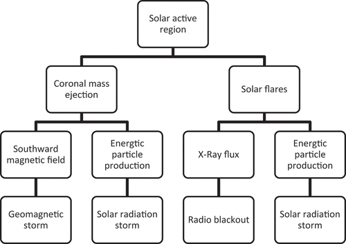
Space infrastructure, made up of a diverse constellation of satellites and space stations, is continuously exposed to several small intensity radiation influences broadly falling in three categories viz., (i) galactic cosmic rays from outside the solar system; (ii) solar energetic particles (SEP); and (iii) radiation belt particles trapped inside the Earth’s magnetic field. Continuous exposure to these types of radiation can damage space infrastructure, like the Earth observation satellites from the Indian Regional Navigation Satellite System (IRNSS) and global positioning systems (GPS), as well as space-based telescopes like Astrosat and Hubble (Cannon et al., 2013). Solar activity may give rise to solar flares from three regions, viz., Alpha, Beta and Delta. Major solar flares tend to occur from the Beta or Delta regions. However, not all Beta or Delta groups produce a flare (Priest, 2014; Table 1).

Table 1. Classifications of sunspots or active regions.

Sunspot Class	Description of the Active Region	Potential for Solar Flare Activity
ALPHA	Unorganized, unipolar magnetic fields	Little threat, but watched for further growth
BETA	Bipolar magnetic fields between sunspots	C class flares and possible M class flares
DELTA	Strong, compact bipolar fields between sunspots	High potential for large M or X class flares

Resultant SEPs have high potential to damage our interests, as they induce changes in total electron content (TEC) values (Eastwood et al., 2017) during solar flare activity from Delta regions. TEC indicates the number of electrons present and measured in electrons per square metre. By convention, 1 TEC Unit (TECU) = 10¹⁶ electrons/m². Value of TEC Ionosphere varies due to factors like solar flares, extreme ultra-violet radiations and geomagnetic storms, as well as atmospheric waves propagating up from the lower atmosphere. Sudden changes in TEC value have various impacts such as:

• Concentration of TEC at detector ecosystem and higher levels can damage the instrument or reduce its life.

• Influence satellite drags, particularly for those in LEO.

• Higher TEC along the path between a radio transmitter and receiver can affect radio waves and result in distraction/decay of signals, significantly affecting the communication between ground and satellite, as well as satellite navigation.

Data from NASA’s Kepler Spacecraft suggests that super-Flares (10x Carrington) may occur on millennial timescales and the probability of a flare in the next 30 years, whose strength broadly exceeds from the flares that were observed in 2003, is only 10% (Shibayama et al., 2013). But there is a growing realization that the vulnerability of space infrastructure is from both ‘low-frequency, high-impact’ events, as well as smaller flare activities (Schrijver et al., 2015). Additionally, SEP during solar flare events can impact the quality of data transmitted from the satellite, hampering precision applications based on GNSS. Changes in the path and velocity of radio waves in the ionosphere have a big impact on the accuracy of satellite navigation systems such as GNSS. Neglecting changes in the ionosphere, TEC can introduce tens of metres of error in position calculations (Hernández-Pajares, 2011; Olga & Natalia, 2016). Further, stresses from space debris are a constant threat to the space infrastructure (Table 2).

Table 2. Potential influence of solar flares.

Ecosystem	Sector	Aspect	Incidents of Damage	Reference
Direct impacts of higher TEC
Outer space	Space infrastructure	Sensitivity	Anomalies (malfunctions) in 10% of satellite fleet during 2003	Cannon et al. (2013)
		Longevity/damage to satellite	ESA satellite, SOHO blinded, October 2003	Marov and Kuznetsov (2014)
	Space applications	Signal decay Signal distraction	Anomalies	Horne et al. (2018); Baker (2001)
On ground	Tele-communications	Mobile networks	Blockage	Eastwood et al. (2017)
	GNSS	Dilution of precision
	Power grid	Grid collapse	Quebec electric power system, 1989
	Aviation	Navigation problems
Indirect effects of higher TEC
On satellite path	Increase drag	Course correction and fuel consumption	Course correction of Galileo and moving ISS	Oliveira and Zesta (2019)
Increased chances of collision	Debris orbital change	Chances of collision with debris damages to instruments; Forced orbit/course correction		Cannon et al. (2013)

Precision is a crucial element for navigation. The precision of the IRNSS signal depends on factors like dilution of precision, clock related errors, multipath errors and so on. Dilution of precision (DOP) is a dynamic factor and needs to be under constant check as it can happen in different forms, viz.:

Horizontal dilution of precision (HDOP)

Vertical dilution of precision (VDOP)

Positional (3D) dilution of precision (PDOP)

Time dilution of precision (TDOP)

Geometric dilution of precision (GDOP)

These DOP can be related as:

PDOP² = HDOP² + VDOP²

GDOP² = PDOP² + TDOP²

SEPs generated during solar flares can influence every aspect of precision and can affect entire ecosystems of GNSS based applications (Oliveira et al., 2018; Eastwood et al., 2017; Figure 2).

Figure 2. Dilution of precision.

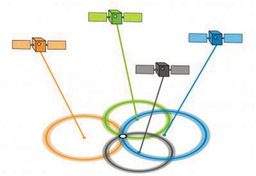
Moreover, the number of satellites operating in LEO and MEO are increasing and all of them are vulnerable to solar flares (Behrens, Lal & Behrens, 2019). Hence every payload should consider variations of TEC for two reasons:

1. To ensure the estimated life span of a payload. For instance, with the rare exception of Hubble, no arrangements are made to rectify instrument failure after launch. Hence, the need for fool-proof protection from these hazards.

2. To ensure signal strength and precision for GPS components.

2. Objectives of the study

Solar Flares (X2.7) of M Category were reported on 12 May 2015 and they were expected to influence the TEC values and GDOP precision. Hence, the study investigates the extent of the influence of solar flares on earth-based applications like geographical dilution of precision (GDOP) and the increase in charged particle concentration (CPC).

Figure 3. Image of an X2.7 solar flare (visible on left side of sun) on 5 May 2015.

3. Methodology

In 2015, incidents of solar flares were higher than average, so monthly data on solar flares in 2015 were obtained from ISRO. A flare with intensity of X2.7 on 12 May 2015 was chosen for the analysis. TEC values were sourced from Byalalu Monitoring Centre of ISRO and variations in TEC were calculated using following formula (Annexure 1).

Total Electron Content (TEC): TEC = 4.4192 [P₂-P₁] (TECU),

(Where 1 TECU (Total Electron Content Unit) = 10¹⁶ el/m²⁾

$GDOP=\frac{\mathrm{\Delta }Outputlocation}{\mathrm{\Delta }Measureddata}$

4. Results

Using the data from ISRO, deviations in TEC were measured (Figures 4 & 5). A distinct spike in TEC was noted and the extent of the spike varied with the locations of satellites. The highest TEC was found in IRNSS No. 1 (TEC 1), where the TEC level was 9.34 × 10²⁰. The second highest TEC was recorded by IRNSS No. 2 (TEC 2) with a TEC of 7.33 × 10²⁰. The lowest spike in TEC was observed in IRNSS No. 4 (TEC 4) and is expected as this satellite was the furthest from the influence of solar flares.

Figure 4. Variation in TEC values registered on 12 May 2015 (X axis = Hour of the day; Y axis = TEC value).

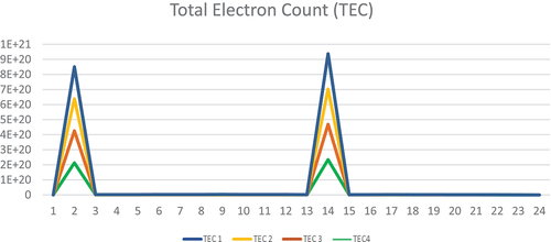
Analysis suggests value of TEC peaks at two points i.e., at 2.00am and 2.00pm, seem to cause subsequent dilution of precision.

Figure 5. Values recorded by IRNSS satellites on 12 May 2015.

5. Measures to safeguard

For GNSS, the distortion or dilution of the precision of the navigation signal is proportional to the TEC value of the ionosphere in each region. For making an estimation of TEC, various models have been developed, viz.:

1. Global level: coefficient based single frequency Klobuchar model and its refinement in the form of global Klobuchar ionospheric coefficients; the Taiwan ionospheric model (TWIM); international reference ionosphere (IRI); and global ionospheric map (GIM). With the help of these models, preventive measures could be initiated.

2. Regional: grid based models such as the minimum mean square error model, the inverse distance weighted (IDW) with the Klobuchar model, the planar fit model, the spherical harmonic function (SHF) model, the modified Klobuchar model for two shell model, and the anisotropic IDW with jack-knife would help in preparedness.

3. For Earth based grid systems: massive corona mass ejections (CME) create disturbances in Earth’s magnetic field and may result in geomagnetically induced current (GIC). A node-by-node forecast of GIC and disconnecting most vulnerable transformers may result in temporary block-out during the storm but would save the grid.

6. Conclusions

Space infrastructure is increasing rapidly, making it more compact and vulnerable to space weather and objects. For the protection of space infrastructure,a few measures may be explored, for instance:

• Space shielding by appropriate materials is worth considering, but the resultant weight could limit its usage.

• Use of magnetic shielding wherein particles are deflected by means of Lorentz force for LEO infrastructure.

Acknowledgments

The author is thankful for the support received from ISRO and the Byalalu Centre, Bengaluru for providing data. Guidance provided by Dr Raju Garudachar and other faculty members at the Department of Aerospace, Jain University Bengaluru, India, are duly acknowledged.

Disclosure statement

The DRI Technical Conference 2022 was sponsored by CDRI, along with editorial work of the Conference Proceedings. However, CDRI did not influence the research, data, findings, and views presented in the research papers.

Water stability test: a tool to assess resilience of geotechnical structures to flooding and water inundationCONTACT Kannan K. R Iyer [email protected] [email protected] [email protected] [email protected] [email protected] [email protected]

ABSTRACT

Safety and stability of geotechnical structures are crucial for ensuring well-performing and resilient infrastructure. Heavy rainfall-induced flooding/water inundation can cause significant damage/failure of geotechnical structures such as road and railway embankments, soil slopes and earth retaining structures. Water inundation/overtopping of geotechnical structures can result in internal/external erosion in soil, collapse of submerged soil and reduction in strength/stiffness. Evaluation of the resilience of stabilized soil against temporal deterioration under water inundation conditions is important. Water stability tests/studies such as crumb tests and soil sensitivity tests have been utilized for dispersive soils and marine soils. However, a water stability test, as a tool for assessment of soil stability, has not gained much attention. This study presents a methodology to evaluate the performance of unstabilized and stabilized marine soil/landfill mined waste, and controlled low strength material inundated in fresh water, saline water and acidic water. The performance of a specimen is evaluated through crumb tests, and microstructural imaging before and after crumb tests. The study demonstrates that biostabilized landfill mined waste exhibits high resistance to inundation conditions. Further, the methodology can be useful for studying the effectiveness and resilience of soil stabilization methods, to develop robust, low-maintenance and sustainable infrastructure for the future.

KEYWORDS:

• Biostabilization
• crumb test
• deterioration
• inundation
• resilient geotechnical structures
• water stability

1. Introduction

Water inundation and flooding causes severe deterioration and damage to infrastructure. Earlier studies have reported damage and failure of embankments, pavements, dams, retaining walls, buildings, bridges and several other important infrastructures due to unexpected floods and water inundation conditions (Elshaer, 2017; Lebbe et al., 2014; Oyediji, Lu & Tighe, 2021; Polemio & Lollino, 2011). Though theoretical assessment of the performance of infrastructure/structures under water submergence and flooding conditions is usually performed, the experimental assessment of water stability of water retaining and other geotechnical structures such as road/railway embankments, and soil slopes has not gained much attention. Such studies can bring great insight into the resilience of geotechnical earth structures (including stabilized soils) to flooding/water inundation. In this context, this study presents a methodology for evaluation of the water stability of unstabilized and stabilized soils/alternate soils.

2. Materials and methodology

2.1. Soil/alternate soil and stabilizers/stabilization methods considered in the study

In this study, three different materials are considered, representing different soil/soil-like materials, i.e., marine soils exposed to saline conditions; landfill mined waste representing the group of industrial/municipal waste materials that can be utilized as alternate soil for fill applications; and controlled low strength material (viz., alternate self-compacting fill material) derived from the combination of natural materials and industrial waste.

The marine soil is collected from the coastal region of Bhavnagar district, located in Gujarat, India. The marine soil has specific gravity of 2.71 and contains 37% clay, 27% silt and 36% sand and is classified as clay with high plasticity (CH). This soil has liquid limits, plastic limits and shrinkage limits of 64%, 31% and 19% respectively, while the presence of salts including Mg, Ca, Na and K (about 20% in oxide form) has been noted in the marine soil (Wanare & Iyer, 2022). The landfill mined waste (LMW) finer than 4.75 mm has been considered in the present study, and has great potential to replace conventional natural soils in infrastructure applications due to its availability in abundance. LMW has specific gravity in the range of 2.28–2.41 and contains mostly sand-sized particles with some gravel, and is classified as SP/SW (poorly graded/well graded sand). The organic content varies from 2–13%. Due to the presence of some residual organic material and possibility of other undesired materials, LMW may need stabilization for its utilization as fill material. Further, the controlled low strength material (CLSM), a self-compacting fill material, has been developed using sand, pond ash, fly ash and cement.

Conventional binders such as cement and lime, as well as sustainable stabilizers/fillers such as fly ash, pond ash, ultrafine slag and GGBS, as well as sustainable methods such as biostabilization, have been employed in the study. Biostabilization has been done by utilizing six different species of Sporosarcina pasteurii bacteria derived in a laboratory from natural soil/LMW samples. The LMW samples were treated for 7 days, 14 days and 21 days duration to understand the effect of treatment duration on its stability, with one dose of bacterial culture and two doses of nutrients per day, wherein 1 M urea and 1 M calcium chloride were used as nutrients.

2.2. Neutral, alkaline and acidic environments

Different environmental conditions such as exposure to normal water (0.01 M NaOH as recommended by BS 1377–5:1990; BSI, 1990), saline water (alkaline sea water conditions) and contaminated water (e.g., acidic exposure conditions) have been considered in the study. Normal water with pH between 8–9, saline water with pH of about 13.30 (1 M NaOH) and acidic water with pH of about 1.80 (1 M H₂SO₄) have been utilized in the study.

2.3. Details of stabilization of soils/alternative soils

Figure 1 shows adopted material combinations investigated in the present study. The nomenclature utilized in Figure 1 is explained with examples. For instance, S20-PA60-FA15-C5-28D for controlled low strength material indicates 20% sand, 60% pond ash, 15% fly ash and 5% cement cured for 28 days. Similarly, SM-U12-L3 indicates stabilized marine soil with 12% ultrafine slag and 3% lime activator. For biostabilized LMW samples, B1 to B6 indicates samples treated with six different bacterial cultures. The different abbreviations utilized for the nomenclature are also explained in Figure 1.

Figure 1. Details of specimens considered in the present study.

2.4. Evaluation of resilience to water inundation by employing crumb tests

Crumb tests and microscopic imaging have been utilized in the study for understanding the stability of the materials under water inundation conditions (Umesh, Dinesh & Sivapullaiah, 2011; Wanare & Iyer, 2022). Three different conditions are considered: normal water inundation representing water inundation due to heavy rainfall, water logging due to discharge of water from dams, overflowing of rivers and lakes and so on; saline water inundation representing inundation of coastal structures in sea/near shore; and inundation under acidic water conditions, representing conditions of high contamination, such as mine tailings.

The specimens were subjected to water inundation of up to 24 hours under different environments (normal/alkaline/acidic), and their behaviour was observed with respect to time (viz., immediately after inundation, 2 min, 30 min, 1 hr, 2 hr, 6 hr and 24 hrs). Figure 2 briefly represents the details of the crumb test (Wanare & Iyer, 2022). The specimens were an approximate cube of 15 mm (with some tolerance to variation in the actual dimensions of the specimen) and were prepared and inundated in water (normal/alkaline/acidic). The stability of the specimens was observed at different time intervals by taking images and the specimens classified as unstable, stable or uncertain based on their water stability response. Unstable specimens exhibited complete disintegration or significant disintegration, while stable specimens did not exhibit disintegration/deterioration. The uncertain specimens showed some disintegration/deterioration, and their stability may depend on the duration and severity of exposure conditions.

Figure 2. Details of crumb tests utilized for water stability assessment.

3. Results and discussions

3.1. Water stability assessment through crumb tests and microscopic imaging

Figure 3 shows compiled crumb test results for unstabilized and stabilized soil as well as alternate soils (viz., landfill mined waste and controlled low strength material). Observations indicate that marine soil is unstable when inundated in normal water, alkaline water or acidic water. (As an example it was observed that marine soil disintegrated within 2 min of normal water inundation and completely collapsed in less than 30 min). The disintegration of marine soil microstructure due to water inundation can be attributed to the reduction in suction due to submergence (suction can be understood as energy with which water is bonded within the soil matrix and contributes to the pseudo strength and stability of soil). As soil gets saturated (viz., all soil pores are filled with water), interaction between different water molecules reduces the capillary surface tension forces within the soil pores, and hence causes reduction in suction as well as cohesion/frictional resistance between soil particles. Similar behaviour is also exhibited by unstabilized landfill mined waste (LMW). The presence of exchangeable Na+ ions in marine soil could contribute to its faster disintegration due to the affinity of the Na+ ions towards water and the development of repulsive forces between soil particles, which disintegrates the soil structure (Umesh, Dinesh & Sivapullaiah, 2011). Stabilization of marine soil and landfill mined waste may contribute towards improving their stability to disintegration.

Further, the water inundation studies on stabilized marine soil (Figure 1) revealed that SM-U7-L3 (stabilized marine soil with 7% ultrafine slag and 3% lime activator) and SM-U12-L3 showed stable behaviour under normal water inundation (Figure 3). However, SM-U7-L3 disintegrated under exposure to both alkaline and acidic conditions, which is mainly caused by the dissolution of cementitious gels that bind the particles together (Zhang et al., 2021). SM-U12-L3 retained stability under all the environmental conditions (normal, alkaline and acidic conditions), and hence provide an optimized combination for marine soil stabilization under water inundation/flooding conditions in the study. Similarly, crumb test results for LMW are summarized in Figure 3. Unstabilized LMW is unstable under normal, alkaline and acidic conditions, mainly due to a negligible fines content, which results in low cohesion between particles. However, biostabilized LMW and stabilization of LMW with 10% cement/lime showed good resistance to water inundation, and specimens were stable under normal, saline and acidic water inundation conditions. However, stabilization with fly-ash cement and GGBS-cement resulted in an uncertain state for a 7-day cured specimen and a stable state for a 28-day cured specimen under normal water inundation. Lime is noted as a better activator for GGBS than fly ash, with lime-GGBS combinations exhibiting stable responses, while lime-fly ash combinations were unstable under normal water environments. Typical crumb test results for some specimens are presented in Figure 4.

Further, landfill mined waste (LMW) stabilized with fly ash and GGBS was observed to be unstable in alkaline and acidic conditions. This could be attributed to the leaching of chemical compounds in the fly ash and GGBS stabilized soils under acidic and alkaline conditions. In contrast, the biostabilized landfill mined waste performed better than stabilization with admixtures, as microbial stabilized samples were stable under all pH conditions (normal, alkaline and acidic).

Figure 3. Water stability responses of various specimens of unstabilized and stabilized soil/alternate soils.

Figure 4. Typical crumb test images for marine soil, landfill mined waste and controlled low strength material specimens.

The stability of biostabilized LMW resulted from reduced porosity within the specimen and precipitation of calcite by microbial species (Figure 5) that do not dissolve in water under different conditions. Hence, biostabilized landfill mined waste is expected to exhibit better performance and higher resistance to flooding and water inundation conditions for different infrastructure applications. In general, biostabilized fill material can reduce the possibility of various challenging conditions such as slope failures, erosion and collapse/subsidence of soil, a reduction in bearing capacity, an increase in settlement of infrastructure facilities and the functional failure of embankment/dykes. Biostabilization can find application for flood protection structures such as sea walls, flood protection bunds, avalanche protection structures, check dams and construction of new lakes to enhance protection against hydrological/inundation hazards.

Figure 5. Crumb test results and microscopic images of biostabilized landfill mined waste.

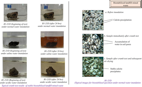
Similarly, crumb tests for controlled low strength material (CLSM) showed stable behaviour in normal and alkaline environments. CLSM showed superior performance as compared to marine soils and landfill mined waste. However, all CLSM specimens were unstable in acidic environments, mainly due to the dissolution of cementitious gels at lower pH. As acidic conditions are not generally expected in most infrastructure facilities, CLSM is suitable for infrastructure applications as a self-compacting fill material; compacting soils due to site access or space constraints is challenging wherever (Dalal et al., 2022).

3.2. Correlation between water stability and strength for normal water inundation conditions

Unconfined compressive strengths were evaluated for different specimens of controlled low strength material and unstabilized/stabilized landfill mined waste, and compared with the corresponding crumb test results under normal water inundation (Figure 6). The observations suggest that, in general, the specimen that exhibits unconfined compression strength ($UCS)\ge 0.2MPa$ shows stable behaviour, while $UCS<0.2MPa$ indicates an unstable response.

Figure 6. Correlation between unconfined compression strength and crumb test results.

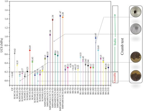
4. Future scope

The present study demonstrates the application of water stability tests for assessing the performance of unstabilized/stabilized soils/alternate soils under different water inundation conditions for geotechnical structures. The study can be further extended to (i) simulate responses of geotechnical structures to cycles of wetting/drying; (ii) assess the erodibility of the structures caused due to flash floods/heavy rainfall; and (iii) evaluation of the resistance of geotechnical structures to water inundations, including long-term exposure.

5. Conclusions

The study demonstrates a combination of crumb tests and microscopic imaging as a tool for the assessment of the water stability of unstabilized and stabilized soils/alternate soils. The research concludes:

• Marine soils and landfill mined waste are unstable in different water inundation/flooding conditions, mainly due to the presence of Na+ ions and lower cohesion/lack of bonding between particles in water submerged conditions. The controlled low strength material (CLSM) exhibits good resistance to normal and alkaline water inundation, while CLSM is unstable in acidic environments due to the dissolution of cementing compounds at lower pH. CLSM may be suitable for most infrastructure facilities with exposure to saline water.

• Correlation between unconfined compression strength (UCS) and crumb tests suggests that under normal water inundation conditions the soil specimen with UCS value > 0.2 MPa exhibits good water stability, while UCS value < 0.2 MPa indicates specimens are unstable with water inundation.

• LMW stabilized with 10% of cement/lime has shown stable behaviour under normal, alkaline and acidic water inundation. However, LMW stabilized with lime-GGBS admixture has shown stability only under normal water inundation, while lime-fly ash has not been effective in ensuring water stability of a LMW specimen. Biostabilized landfill mined waste showed most stable performance when water inundated at various pH. As this method is environmentally friendly, biostabilization can be a suitable soil stabilization method that may contribute to developing resilient infrastructure facilities against flooding/water inundation.

Acknowledgments

Sincere gratitude is extended to the Gujarat State Biotechnology Mission (GSBTM), Department of Science and Technology, Government of Gujarat, India, for funding an ongoing research project (Project ID: L1Y5SU) on ‘Bio-stabilization and Reutilization of Non-biodegradable Fraction of Municipal Solid Waste for Various Civil Engineering Applications’.

Disclosure statement

The DRI Technical Conference 2022 was sponsored by CDRI, along with editorial work of the Conference Proceedings. However, CDRI did not influence the research, data, findings, and views presented in the research papers.

Earthquake response control of hospital buildings using unbonded fibre-reinforced elastomeric isolatorsCONTACT Sarranya Banerjee [email protected] [email protected]

ABSTRACT

Lifeline structures such as hospital buildings need to be specifically designed such that they experience low levels of vibration when subjected to earthquake excitations. This is necessary since it is not easy to evacuate hospital buildings during earthquakes. This study aimed to utilize flexible unbonded fibre-reinforced elastomeric isolators (UFREIs) for seismic isolation of an existing eight-story hospital building in New Delhi, India, to achieve minimal dynamic response of the structure under seismic excitations. Recently, the authors have proposed a novel trilinear hysteretic model (THM) to represent the force-deformation behaviour of UFREIs, which could effectively predict the highly nonlinear behaviour of UFREI using only four design parameters. Although THM has shown considerable promise in modelling the dynamic behaviour of UFREI, it is yet to be implemented in the response evaluation of actual UFREI-isolated structures. Thus herein, detailed properties of UFREIs installed in the considered hospital building are obtained utilizing the proposed THM under a site-specific design scenario. Numerical analyses of UFREI-isolated hospital buildings are also conducted. The UFREI-isolated hospital building is subjected to an ensemble of site-specific earthquake excitations and responses of the structure are obtained using the novel THM of UFREI. Response parameters of the UFREI-isolated hospital buildings such as top-floor structural acceleration, inter-story drifts of the structure and force-deformation behaviour of UFREIs are evaluated to demonstrate the performance of UFREI-isolated hospital building under selected ground motions. The results established the effectiveness of UFREIs for seismic isolation of building structures.

KEYWORDS:

• Base isolation
• earthquake
• hospital building
• unbonded fibre-reinforced elastomeric isolators
• vibration control

1. Introduction

Base isolation systems (BISs) are vibration control devices popular for reducing structural seismic responses when subjected to strong earthquake excitations (Matsagar & Jangid, 2008). Fibre-reinforced elastomeric isolators (FREIs) are innovative emerging elastomeric isolation systems constructed by bonding alternate layers of rubber and fibre reinforcement (Kelly, 1999). FREIs are considerably lighter in weight compared to conventional steel-reinforced elastomeric isolators, making installation and maintenance of FREIs much convenient and economical. In unbonded applications, FREIs are placed in between the superstructure and substructure without being explicitly attached to them. This allows FREIs to be much more flexible due to their unique rollover deformation (Toopchi-Nezhad, Tait & Drysdale, 2011). Due to these significant advantages, many researchers have investigated the dynamic behaviour of unbonded FREIs (UFREIs), both experimentally and theoretically (Banerjee & Matsagar, 2022; Ngo, Deb & Dutta, 2018; Toopchi-Nezhad, Tait & Drysdale, 2008). Banerjee and Matsagar (n.d.) have also proposed a novel trilinear hysteretic model (THM) for representing the horizontal force-deformation behaviour of UFREIs. THM provides efficient means to design UFREIs incorporating site-specific conditions. The performance of UFREIs are also established for isolating low-rise structures against earthquake excitations (Das, Deb & Dutta, 2016; Thuyet, Deb & Dutta, 2018; Toopchi-Nezhad, Tait & Drysdale, 2008).

Usually, BISs are designed to shift the fundamental time period of a structure to around 2–3 s, which efficiently reduces a superstructure’s vibration such that no or minimal damage is caused during an earthquake event. However, lifeline structures such as hospital buildings need to be serviceable even during strong earthquake excitations. Therefore, it will be beneficial to design very flexible isolation systems for important structures to reduce the superstructure response further. Literature reveals many examples of hospital buildings retrofitted with various BISs (Ferraioli & Avossa, 2012; Ferraioli & Mandara, 2017), however UFREIs are not yet utilized for base isolation of hospitals. Thus, the objective of this study is to investigate the performance of UFREIs in controlling seismic responses of an existing eight-story hospital building in Dwarka, New Delhi, India. In addition to demonstrating the efficacy of UFREIs, this article also illustrates a technique for the utilization of UFREIs in relatively tall structures, thus not restricting its use to only ordinary low-rise structures (Toopchi-Nezhad, Tait & Drysdale, 2008). To achieve these objectives, first the eight-story hospital building is idealized as a multi-degree-of-freedom (MDOF) shear building model. Subsequently, a flexible isolation system with isolation period of 4 s is designed for the considered structure, using the design procedure suggested by Banerjee and Matsagar (n.d.). Further, nonlinear equations of motion of the UFREI-isolated hospital building are numerically solved to obtain its response under select site-specific earthquake excitations. Finally, the effectiveness of the proposed UFREI system in reducing seismic responses of the hospital building is established.

2. Modelling of the hospital building

This study investigates the seismic performance of a ward block of an existing hospital in Dwarka using UFREIs for its base isolation. Figure 1 shows details of its plan, the structural members, and their placements on a typical floor of the ward block. Isolators are placed at ground level and the required moat width is maintained around the ground for its proper functioning. The heights of the first two stories, the top story and other remaining stories are 4.05 m, 3.85 m and 3.9 m, respectively. The 28-day characteristic compressive strength of the concrete of beams and slabs is 25 MPa, and of columns and shear walls is 30 MPa.

Figure 1. Typical floor plan and structural details of the hospital building in Dwarka, New Delhi.

Interiors of the hospital building include partitions with 100 mm thick fly-ash brick walls and a 75 mm thick floor finish. Twenty-five percent of 2 kN/m² imposed load is considered to be acting on each floor of the structure during any earthquake event (IS 875 (Part 2): 1987, 1987). All these factors are considered and the multi-story hospital building is idealized as a multi-degree-of-freedom (MDOF) shear building model with its masses lumped at each floor level. With this, the fundamental time period of the MDOF structure is obtained as 0.3714 s in the x-direction, and its damping ratio is assumed to be 2%.

3. Design of an UFREI-based isolation system for the hospital building

Seismic isolation of the hospital building is carried out using UFREIs with the help of the THM proposed by the authors. Figure 2 shows the normalized THM indicating its parameters to estimate force-deformation behaviour of an UFREI with any geometrical or material properties. From Figure 2, the effective stiffness and effective damping ratio of THM could be computed by equivalent linearization. Hence, based on certain given site-specific conditions, the UFREIs are designed for the required isolation period. The detailed design procedure is available in Banerjee and Matsagar (n.d.).

Figure 2. THM for representing the force-deformation behaviour of UFREIs (Banerjee & Matsagar, n.d.).

The hospital building is isolated with an isolation time period of 4 s. Existing literature on UFREIs (Das, Deb & Dutta, 2016; Ngo, Deb & Dutta, 2018; Toopchi-Nezhad, Tait & Drysdale, 2008) suggests that the vertical pressure carrying capacity of UFREIs is considerably lower than other base isolators. Due to this property, UFREIs are preferred in low-rise structures having relatively small vertical loads. Therefore, to install UFREIs in the eight-story hospital building, free sliders are also used to transfer the vertical loads from the superstructure to the foundation. Free sliders are manufactured from polytetrafluoroethylene (PTFE) coated steel plates which could efficiently transfer the vertical load without providing any lateral restoring force to the structure under horizontal displacements (Ferraioli & Mandara, 2017).

In addition to the isolation period and vertical pressure, UFREIs have to be designed for a specific design displacement. Therefore, the design displacement of the UFREI-isolated hospital building is decided by computing the maximum displacement of the isolators when the isolated structure is subjected to site-specific maximum considered earthquake (MCE) ground motions (details are provided in the following section). In the present scenario, design displacement is calculated and checked iteratively to be 340 mm. However, for an additional factor of safety, the UFREIs are designed to be stable under horizontal displacements of 480 mm. With this, Figure 3 shows the details of a single UFREI placed under the superstructure for base isolation of the hospital building. Figure 4 shows the entire layout of the isolation system, depicting types and numbers of isolators being used. As seen from Figure 4, the free sliders are directly fixed under columns to transfer the vertical loads of the superstructure; UFREIs are placed slightly away from the columns and are not designed to carry any vertical load from the superstructure. The height of free sliders is 4.5 mm less than the UFREIs to maintain sufficient vertical pressure on the UFREIs for its proper functioning.

Figure 3. Properties of a single UFREI utilized for base isolation of the hospital building.

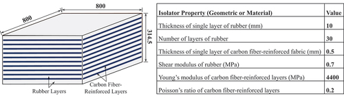
Figure 4. Plan layout and details of the UFREI-based isolation system.

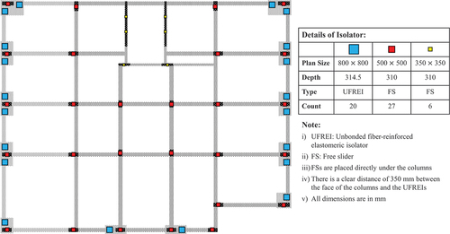
4. Performance of UFREI-isolated hospital building

The performance of the hospital building with the proposed isolation system (Figure 4) is tested under various site-specific earthquake excitations. Eight different strong recorded ground motions are selected and they are scaled suitably such that they resemble site-specific earthquake scenarios in New Delhi, India for the MCE condition. The design response spectrum is selected form IS 1893 (Part 1): 2016, with importance factor of 1.5, response reduction factor of 1, and a multiplicative factor of 2 for converting the design spectrum from design basis earthquake (DBE) condition to MCE condition. The recorded earthquake excitations are scaled to match their response spectrum with the target (design) spectrum using a computer software, SeismoMatch (2022). Details of the selected earthquakes are provided in Table 1.

Table 1. Details of site-specific earthquake excitations considered in this study.

Notation	Earthquake Name	Year	Recording Station	Component	Original PGA (g)	Scaled PGA (g)	Duration (s)
EQ1	Imperial Valley	1940	El Centro	00	0.341	0.406	53.760
EQ2	Kern County, CA	1952	Taft Lincoln School Tunnel	TAF111	0.176	0.553	54.400
EQ3	Kobe	1995	JMA	NS	0.818	0.488	150.000
EQ4	Loma Prieta	1989	Los Gatos Presentation Centre	90	0.596	0.476	25.005
EQ5	Mexico City	1995	Station 1	180	0.168	0.443	180.120
EQ6	Northridge	1994	Sylmar Converter Station	360	0.827	0.517	60.000
EQ7	San Fernando	1971	Pacoima Dam	S74W	1.054	0.451	41.720
EQ8	San Francisco	1957	San Francisco Golden Gate Park	S80E	0.102	0.418	39.880

Next, the UFREI-isolated hospital building is subjected to the selected site-specific, unidirectional ground motions (Table 1). The performance of UFREIs in controlling seismic responses of the structure is investigated. The force-deformation behaviour of the UFREIs is modelled using the THM; the response of the structure is evaluated by numerical integration of the nonlinear equations of motion of the UFREI-isolated MDOF building model, using the 4^th-order Runge-Kutta method. Figure 5 shows top-floor absolute acceleration responses of the structure with and without base isolation. The time–history responses shown in Figure 5 are truncated for better visibility of regions with severe vibration. It is observed that the top-floor accelerations in the UFREI-isolated building reduces significantly with the proposed flexible isolation system, making the hospital building serviceable even during the earthquake. Similar to peak acceleration responses, the peak base shear of the hospital building is also reduced by 91–94% (results not shown here).

Figure 5. Time history of top-floor absolute acceleration responses (truncated) of hospital building with and without base isolation.

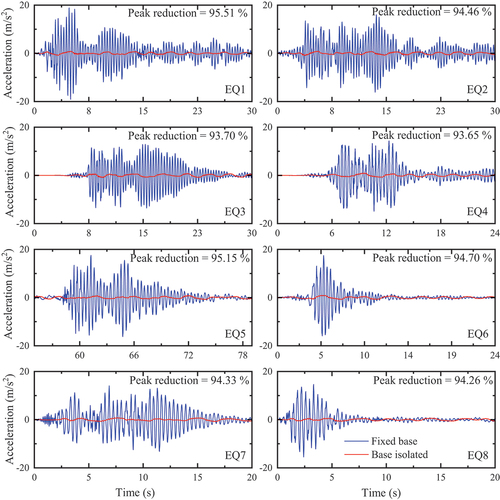
Figure 6 shows peak inter-story drift ratios of all the stories of the hospital building. The UFREI-based isolation system has been able to reduce the peak inter-story drift ratios of the structure by 91–94%. This demonstrates the effectiveness of the UFREIs in isolating the selected building.

Figure 6. Peak inter-story drift ratio of the hospital building with and without base isolation.

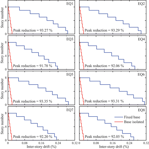
Figure 7 shows the force-deformation behaviour of the UFREIs under various earthquake excitations. The effective stiffness of the isolators is evaluated by equivalent linearization (Banerjee & Matsagar, n.d.). The design displacement of the UFREIs was obtained as 340 mm, however the isolators did not displace to that limit under all the earthquakes. Therefore, the effective isolation periods in all the cases are found to be lesser than the design isolation period. Under some earthquake excitations, the isolator displacement did not cross the second yield point in the THM, thus displaying a bilinear hysteretic behaviour. Irrespective of these factors, the UFREI-based isolation system is effective in reducing seismic responses of the hospital building, under all the earthquake excitations.

Figure 7. Force-deformation behaviour of the UFREI-based isolation system using the THM.

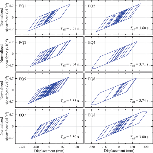
5. Conclusions

UFREIs are innovative seismic isolators which could constitute very flexible isolation systems for various types of structures. In this paper, a UFREI-based isolation system is designed for a real-life hospital building situated in New Delhi, India. Comprehensive design of the isolation system is carried out utilizing the design procedure previously developed by the authors. The force-deformation behaviour of the UFREIs is represented using the THM, and responses of the UFREI-isolated hospital building are evaluated. The results showed that the UFREI-based isolation system is very effective in reducing responses of the hospital building under site-specific earthquake excitations of MCE condition. The peak top-floor acceleration response, peak base shear as well as the peak inter-story drifts of the isolated structure are reduced by 91–96% under all the test earthquake excitations. The force-deformation behaviour of the UFREIs show that the flexible isolation system could achieve isolation time periods in the range of 3.5 s to 3.8 s, under different earthquake scenarios. These results demonstrate that the UFREI-based isolation system can significantly reduce the seismic responses of building structures. Such isolation systems are necessary to ensure serviceable conditions inside important structures such as hospital buildings even during severe earthquakes.

Acknowledgments

This research work is funded under the Coalition for Disaster Resilient Infrastructure (CDRI) Fellowship Programme, awarded to Prof. Tracy Becker, Department of Civil and Environmental Engineering, University of California and Vasant Matsagar; the financial support is gratefully acknowledged. Nevertheless, the opinions expressed and findings reported in this document are that of the authors only and not of the funding agency.

Disclosure statement

The DRI Technical Conference 2022 was sponsored by CDRI, along with editorial work of the Conference Proceedings. However, CDRI did not influence the research, data, findings, and views presented in the research papers.

Adaptive pathways for disaster-resilient infrastructure: resilience assessment as a fundamental requirementCONTACT Mohammad Rafiq Joo [email protected] Sinha [email protected].

ResearchGate: https://www.researchgate.net/profile/Mohammad-Rafiq-4

LinkedIn: https://www.linkedin.com/in/mohammadrafiqmr/

ABSTRACT

Built infrastructure must be resilient to prevail in the face of disasters. Adopting strategic options and policies for disaster risk mitigation and community resilience enhancement are conditioned on accurate, comprehensive and systematic disaster risk assessment of infrastructure. The pathways promote incremental adaptation and consider post-disaster requirements through a proper resilience assessment. Such an approach is a prerequisite for implementing pathways for disaster-resilient infrastructure but is currently not prevalent. The present study carries out resilience assessment from a seismic risk reduction consideration, incorporating functionality loss and subsequent recovery for a representative archetypical commercial building. Various scenarios of pre- and post-disaster preparedness, planning and mitigation options are considered to provide deeper understanding of pathways. Assessments are conducted in accordance with the state-of-the-art performance-based earthquake engineering (PBEE) framework. The results are compared using a range of resilience metrics. The impact of an engineering intervention, viz., improvement to non-structural performance, a management intervention, viz., mitigation of post-disaster repair impedances, and their combination are demonstrated and quantified. The study shows how various pre-disaster planning, preparedness strategies and post-disaster management options influence resilience and that they can be combined to enhance infrastructure resilience. Multiple options are presented for efficient decision-making by stakeholders and policymakers to deal with uncertainties during disasters. The study advocates embracing the resiliency mindset and involving multiple stakeholders in risk-informed decision-making.

KEYWORDS:

• disaster-resilient infrastructure
• adaptive pathways
• resilience assessment
• functional recovery
• post-disaster management

1. Introduction

Disasters have a massive economic and social impact, disrupting essential services and displacing individuals and businesses (Potter et al., 2015). In the post-disaster phase, significant uncertainties are encountered in efforts to restore functionality of the infrastructure. A disaster-resilient system aims to withstand some of a disaster’s impacts, maintain a minimum functionality level, restore quickly and better adapt and improve for future hazards (Kurth et al., 2019). The concept and implementation of resilience provides avenues to investigate solutions to various important concerns in the infrastructure industries (UNDRR, 2022).

Adaptation refers to the system’s evolution to become more resistant to and recoverable from future disasters. Adaptive pathway is a promising decision-focused analytical approach for exploring and sequencing a set of actions to reduce future risks, incorporating flexibility into planning and decision-making while also accounting for future uncertainties (Haasnoot et al., 2013). Studies (Djalante et al., 2013; UNDRR, 2022) recognize disaster risk and impact assessments as essential for identifying system vulnerabilities and opportunities for future adaptation. A comprehensive and systematic assessment of hazard, risk, vulnerability and impacts is required to develop pathways for adaptive and integrated disaster resilience (Djalante et al., 2013). However, conventional risk assessment frameworks are based on a narrow perspective and do not incorporate recovery and future adaptation. Past choices and decisions affect the adaptation options and available trajectories today, and need to be considered (Tellman et al., 2018). The pathways focus on incremental adaptation; therefore, resilience assessments incorporating post-disaster recovery parameters are critical to reduce future losses. In addition to conventional loss and risk assessments, functional recovery assessment is an integral contributor to disaster-resilient infrastructure and a fundamental requirement for successfully implementing adaptative pathways.

The present study quantitatively evaluates various strategies and control measures to limit financial losses and building downtime due to earthquake risk, thereby linking the present situation to pathways for more resilient infrastructure. Resilience assessments for a representative building under different scenarios of pre- and post-disaster measures are carried out to identify the root causes of future risks and the opportunities to address them efficiently. Performance is assessed and compared using a range of resilience metrics, including reoccupancy and functional recovery times, scenario losses, repair times, likelihood of red (unsafe) tags and probability of collapse. The effects of various non-structural performance improvements, mitigation of post-disaster delays and their combination are explored and quantified. The paper shows how the pre-disaster planning and preparedness strategies, as well as efficient post-disaster management and decisions, can help enhance infrastructure resilience. Various options are presented to stakeholders for efficient decision-making in uncertain disasters. The study encourages embracing the resiliency mindset and engaging multiple stakeholders to exchange information, make risk-informed decisions, conduct greater preplanning, and develop well-coordinated prioritization plans.

2. Resilience assessment methodology

Building-specific resilience assessments are conducted in accordance with the state-of-the-art probabilistic performance-based frameworks (ATC 138–3, 2021; FEMA P-58, 2018). The following subsections provide details about the archetypical building, structural modelling and simulation, damage and loss assessment, and functionality loss and subsequent recovery approaches.

2.1. Building selection, structural modelling and hazard estimation

A seven-story reinforced concrete (RC) archetypical building (ID-2215), designed for New Delhi, India, and representing a typical commercial building, such as ones used for governance functions, is selected from Badal and Sinha (2019). Detailed information about the geometric and material characteristics and the member design and detailing is available in Badal and Sinha (2019). For performance assessment, non-structural components for typical office occupancy have been included from the FEMA P-58 (2018) fragility database and the detailed information about the components are available in an extended study (Joo & Sinha, 2023).

A two-dimensional structural model employing concentrated plasticity approach and incorporating P-delta effects was developed in OpenSees (McKenna, Fenves & Scott, 2000) to simulate the nonlinear behaviour of RC frames. The nonlinearity of beams and columns is modelled using zero-length nonlinear flexural hinges, and hysteretic behaviour, at each end. The effects of longitudinal reinforcement bond-slip behaviour, finite beam-column joints and foundation flexibility are also considered (Joo, Badal & Sinha, 2022).

The seismic hazard from a probabilistic seismic hazard assessment for New Delhi, India (28.61°N, 77.21°E), has been used (Raghukanth, 2020). The widely used hazard levels in engineering, 10% probability of exceedance (POE) in 50 years, referred to as design basis earthquake (DBE), and 2% POE in 50 years, referred to as maximum considered earthquake (MCE), were selected. Twenty pairs of ground motions were selected and scaled at each hazard level corresponding to conditional mean spectra. Further details about the selection and scaling parameters are available in Joo, Badal and Sinha (2022).

2.2. Loss and recovery assessment procedure

The storey drift and floor acceleration responses were obtained from nonlinear response history analyses of the RC frames in both horizonal directions. The effect of building non-repairability in case of excessive residual drift was considered using non-repairable fragility function. The residual story drifts were obtained from peak transient interstorey drifts following FEMA P-58 (2018) recommendations.

In this study, the PBEE approach is utilized to assess the damage states, repair costs and repair time of various building components in accordance with the FEMA P-58 approach. Uncertainties in structural responses, damage states, repair costs, impedance and repair times are incorporated through Monte Carlo simulations with 5000 realizations. Building collapse fragility functions are taken from Badal and Sinha (2022), and the component fragility and consequence functions from the FEMA P-58 database. The likelihood of assigning an unsafe placard due to damage compromising life-safety has been estimated based on a virtual inspection process (Cook et al., 2021). The damage assessment results are utilized to evaluate the building’s reoccupancy and functionality immediately, as well as subsequently over time after an earthquake event in accordance with the ATC 138–3 (2021) approach, which is based on the functional recovery framework (Cook et al., 2022). The different impeding factors and the repair-scheduling algorithm are considered to evaluate time required for reoccupancy, functional recovery and full recovery (ATC 138–3, 2021; Cook et al., 2022). The study uses FEMA P-58 and ATC-138 methodologies, which are implemented in SP3 (2022) software.

2.3. Resilient infrastructure pathways

This study selected a benchmark baseline archetypical building to understand different options and pathways for improving infrastructure resilience. Resilience can be improved by engineering measures such as enhancing system robustness (improving structural and non-structural performance), management measures such as mitigating post-disaster impedances, efficiently managing recovery activities, and so on. In the study, the non-structural elements of the baseline model (model ‘a’) were replaced (Joo & Sinha, 2023) with those possessing improved resilience while retaining the same capacity of structural elements (model ‘b’). During the post-disaster period, an inter-disciplinary management group that includes structural surveyors, engineers, designers, contractors and budget-management people can help reduce the post-disaster delays to repairs and thus accelerate recovery. Therefore, having the surveyor, engineer and contractor on retainer and eliminating a long lead time to begin repairs has been investigated in model ‘c’. Finally, a scenario has been considered combining engineering and management options through non-structural performance improvements and mitigation of post-disaster delays, allowing temporary repairs and managing a surge in labour and material demand (model ‘d’).

3. Resilience assessment results and discussions

Assessment results of the different case studies and pathways for infrastructure resilience are described in terms of seismic scenario losses, repair, reoccupancy, and functional and full recovery times in the following subsections.

3.1. Baseline building performance

Collapse or excessive residual drifts were not observed for model ‘a’ under DBE level events confirming the adequacy of the current design practices for the archetypical building focused on life-safety-based principles. At MCE level, the building has 0.3% collapse probability and 3.4% probability of damage beyond reparability. The likelihood of red-tag damage after DBE and MCE are 3.2% and 34% respectively. Table 1 presents the scenario losses, normalized with the building replacement cost and repair and recovery time. The average repair cost ratios, referred to as scenario expected losses (SEL), are 3.2% and 14%, while the median values are 2.2% and 9.5%, for DBE and MCE level, respectively.

Table 1. Scenario losses, repair time and recovery time assessment results.

Hazard Intensity	Model	Scenario Losses (%)			FEMA P-58 Repair Times (days)		Median Recovery Times (days)
		SEL	Median	SUL	Parallel	Series	Reoccu-pancy	Functional Recovery	Full Recovery
10% POE in 50 years (DBE)	a	3.2	2.2	6.9	11	20	0	125	185
	b	1.7	1.0	4.1	3	5	0	3	160
	c	3.2	2.2	6.9	11	20	0	85	140
	d	1.7	1.0	4.1	3	5	0	3	110
2% POE in 50 years (MCE)	a	14	9.5	22	55	95	165	295	330
	b	11	6.1	17	40	55	3	290	300
	c	14	9.5	22	55	95	135	175	245
	d	11	6.1	17	40	55	3	155	185
Notes: a = Baseline Model; b = Improved Non-structural Performances; c = Mitigation of Post-disaster Impedances; d = Improved Non-structural Performances and Mitigation of Impedances; SEL = Scenario Expected Losses; SUL = Scenario Upper Losses; POE = Probability of Exceedance

The results suggest that the building is expected to be immediately occupiable after DBE level events, but will not be habitable for 165 days after MCE level events. On the other hand, the expected (median) functional recovery time (days) for DBE and MCE level events are 125 and 295, respectively. Full recovery to pre-earthquake conditions is expected to take 185 and 330 days for DBE and MCE level events, respectively. Longer downtime adds significantly to indirect losses and presents severe concerns for various stakeholders to enhance resilience. Post-disaster performance improves over time as different components are repaired as shown in Figure 1.

3.2. Non-structural performance improvements

The collapse likelihood, red tag and non-reparability are similar for model ‘b’ as baseline model ‘a’. SEL reduced from 3.2% to 1.7% and 14% to 11% and median losses from 2.2% to 1.0% and 9.5% to 6.1%, for DBE and MCE level events, respectively. The corresponding reductions in SUL values and repair times are also shown in Table 1. The median reoccupancy time for MCE events was observed to be three days, compared to 165 for the baseline model. It is clearly seen that relatively lower damage to non-structural elements helps in quicker functional recovery, with the corresponding median values reducing from 125 to 3 days at DBE level. The improvements in reducing loss of occupancy and functionality immediately and over time after a disaster are shown in Figure 1.

Figure 1. Probability of (a) occupancy loss and (b) functionality loss at DBE and MCE over time for various pathways.

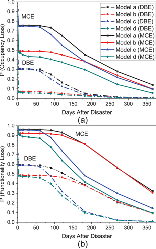
3.3. Mitigation of post-disaster delays

The role of mitigating post-disaster delays in accelerating building reoccupancy and functional recovery is presented in Table 1 (model ‘c’) and Figure 1. The results reveal that controlling post-disaster impedance (time taken to begin repairs) significantly expedites functional and full recovery. As seen in Table 1, the median functional recovery time (in days) reduces from 125 to 85 and 295 to 175, and the full recovery time, in days, from 185 to 140 and 330 to 245, at DBE and MCE level events, respectively. These mitigation strategies do not increase the probability of occupancy or reduce functionality loss immediately after a disaster, but have a substantial impact in the later post-disaster phase (see, Figure 1). The improvements are more pronounced for loss of functionality compared to loss of occupancy.

3.4. Combining pre- and post-disaster measures

As expected, for model ‘d’, the scenario losses, repair times and immediate occupancy and functionality losses are similar to model ‘b’. Remarkably, the median reoccupancy time at MCE level decreases from 165 days to 3 days. Similarly, the median functional recovery time (in days) reduces from 125 to 3 and 295 to 155, while full recovery time, in days, reduces from 185 to 100 and 330 to 185, for DBE and MCE levels, respectively. Six months after the event, the probability of occupancy loss reduces from 5% to 3% and 45% to 30% at DBE and MCE levels, respectively, compared to the baseline model. The probability of functionality losses reduces even more drastically from 38% to 10% at DBE level and 81% to 42% at MCE level, six months after event. Improving non-structural performance during the pre-disaster phase and combining with management intervention to mitigate post-disaster delays contributes the most to resilience improvement (see, Table 1 and Figure 1). It represents the best option for improving performance and achieving modern infrastructure resilience goals among the options considered in this study. Further details about individual options and their impact on resilience metrics are available in a companion study (Joo & Sinha, 2023).

4. Conclusions

The present study presents the resilience assessment for a representative commercial building under various scenarios of pre-and post-disaster actions to evaluate adaptive pathways for disaster-resilient infrastructure. The study considers engineering measures of enhancing resilience of non-structural elements and mitigating delays in undertaking repairs after the event. The study encourages embracing the new resiliency mindset and presents various options to stakeholders and policymakers for collaborative decision-making. The insights gained in this study can also be applied to other infrastructure and disaster scenarios. Some key conclusions from the study are listed here:

• The study extends the concept of integrating scientific information into planning and establishes resilience assessment as a prerequisite for evaluating adaptive pathways for disaster-resilient infrastructure.

• The advantages of considering appropriate engineering measures are shown to significantly reduce functionality loss even though the structural performance remains unchanged. The study underlines the difference between safety and functionality as a design objective and highlights the importance of considering functionality of critical infrastructure.

• The role of management measures to mitigate post-disaster delays in repairs to accelerate the recovery process are quantified. It is shown that mitigating post-disaster delays has a strong positive impact on increasing resilience.

• The study shows that the influence of engineering and management measures to enhance resilience can be investigated under a common framework based on PBEE. The study also shows that the combined benefits of the various measures can also be evaluated. The study further shows that the impact of mitigation measures on resilience over time after the event can also be evaluated and used for pre-event planning.

Acknowledgments

Authors acknowledge the PMRF award to Mohammad Rafiq Joo for his PhD studies at IIT Bombay. The authors also thank the HBRisk group for free academic access to SP3 software.

Disclosure statement

The DRI Technical Conference 2022 was sponsored by CDRI, along with editorial work of the Conference Proceedings. However, CDRI did not influence the research, data, findings, and views presented in the research papers.

An integrated and dynamic approach to assessing risks through capabilitiesCONTACT Andrew Estrain [email protected]; [email protected]

ABSTRACT

Each year, jurisdictions with varying capabilities and vulnerabilities face risk of impacts from hazards. Local and state governments are tasked with hazard planning, analysis and outreach responsibilities to build continuously on emergency preparedness and mitigation efforts to reduce vulnerability to hazard events. A risk assessment (RA) is a major component of the hazard mitigation planning process and includes analyses of risks and potential impacts to the hard infrastructure of a community. This paper goes beyond the risk assessment and argues for supplementing it with a capability assessment framework that will inform mitigation strategies that address the risk to both hard and soft infrastructure. This paper improves the conceptualization of the adaptive pathways that allow planners and policymakers to identify changes as well as their implications within a community. The research assesses soft infrastructure, which enables systems to support the design of hard infrastructure systems to reduce risk and improve resilience. The methodology involves collecting departmental and jurisdictional information about human, physical, technical, explanatory and financial resources through three different surveys and information-gathering tools. The authors provide steps for collecting information on various types of resources, as well as completing an equitable and inclusive capability assessment, through an understanding and strengthening of soft infrastructure. The equitable outreach in the capability assessment process ensures that underserved communities and most vulnerable populations are considered in resource allocation to offset deficiencies in capabilities and capacities in a community.

KEYWORDS:

• Capabilities
• infrastructure
• resilience
• equitable
• assessment

1. Introduction

The frequency and intensity of hazards are increasing across the world, leading to population displacement, deteriorating infrastructure, political instability and increasing demands for government services. Disaster resilience within community infrastructure systems is more necessary now than ever before. Striving for resilience will enable jurisdictions to make risk-driven decisions and ensure flexible and dynamic processes ready for test during ‘blue skies’, as well as in emergency situations.

Each year jurisdictions and communities of all kinds with varying capabilities and vulnerabilities are impacted by hazards. Local and state governments are tasked with an array of hazard planning, analysis and outreach responsibilities to build and support preparedness and mitigation efforts to reduce vulnerabilities continuously. In such complicated and evolving environments, agencies without a holistic and innovative approach may overlook important hazards, underestimate response requirements and lack stakeholder engagement and outreach. This may create an incomplete, or even inaccurate, operating picture of the social, natural, economic and built environment in the area and compromise their overall resilience.

Disaster resilience is defined as the ability of individuals, communities, organizations and states to adapt to and recover from hazards, shocks or stresses without compromising long-term prospects for development. Resilience is determined by the degree to which those individuals, communities and public and private organizations can learn from past disasters and take action to reduce their future risks (GSDRC Applied Knowledge Services, 2022). Resilient communities have sustainable infrastructure, efficient governance, institutionalized planning processes and involve citizens within their information-sharing network. Hard infrastructure is the tangible or built infrastructure, including physical infrastructure such as roads, bridges, tunnels, railways, ports and harbours, among others (Picot et al., 2015). Soft infrastructure includes institutions essential to the economy and quality of life, such as government, health, education, financial and legal systems (Spacey, 2017). This paper focuses on building resilience through soft infrastructure (plans and policies for systems), as well as how effectively to assess a community’s hazard mitigation and preparedness capabilities to reduce risk.

Community risk assessment (CRA) and capability assessment (CA) are two major drivers for the protection of community infrastructure systems. CRA helps identify and analyse potential vulnerabilities and threats to assets, such as building construction, processes, systems, and security and protection systems. CA focuses on examining existing plans, policies and other mechanisms designed to reduce current or future disaster losses. Together CRA and CA determine how effectively a jurisdiction can respond to hazard events. Decision-makers’ poor responses to emergent threats can intensify the vulnerability of their communities instead of mitigating risks. Effects of their responses on system dynamics, robustness and vulnerability can be effectively assessed through an analysis of long-term adaptive pathways, consisting of events, decisions and actions. The assessment will also reveal gaps, weaknesses and strengths of a community’s capabilities.

The concept of ‘pathways’ has gained traction in discourses and policy domains. An adaptation pathway is a decision-making strategy that comprises a sequence of manageable steps or decision-points over time (Coast Adapt, 2017). Adaptive pathways allow decision-makers to explore the need for, and the implications of, societal transitions and transformation. This broadened perspective provides insights and guidance on the interplay between evolving systemic changes and necessities of hazard mitigation. In this paper, we propose a method to conduct CA and an approach to address equitable outreach. To enhance overall risk reduction, this paper goes beyond CRA and focuses on adaptive pathways during or after the CRA is completed. Specifically, the paper argues that development of a CA focused on an inventory of resources and soft infrastructure provides an effective adaptive pathway to enhance resilience for community and infrastructure.

The paper conceptualizes adaptive pathways that allow planners and policymakers to identify the necessity and implications of change within a community. Adaptive pathways diagnose whether systemic change is needed, as well as the role of incremental adaptation in achieving it. They help in awareness and understanding of the interplay among knowledge, values, power and agency to inform responses to change, particularly in dynamic, complex and contested contexts (Wise et al., 2014).

2. Developing the jurisdictional capability assessment

The CA process may be conducted as part of the disaster/hazard mitigation planning process, which can be used to examine and evaluate capabilities and resources in place. Additionally, CA identifies where improvements can be made to increase disaster resistance and enhance resilience.

We analyse Lehigh Valley, Pennsylvania’s Hazard Mitigation Plan (LVHMP), where CA evaluates the existing capabilities of its local jurisdictions to reduce risk through five measures:

• Human resources: local police, fire, ambulance and emergency management and response personnel; local government operation and services; and electricity, gas and other utility providers that need to function during critical periods in disasters.

• Physical resources: equipment and vehicles (such as emergency response and recovery equipment and vehicles); and public land, facilities and buildings available to the community.

• Technical/technological resources: to ensure early warning systems, weather alert radios, stream level monitoring gauges and emergency (911) communications systems are working.

• Explanatory resources: comprehensive available knowledge about disasters and hazard mitigation and planning.

• Financial resources: to ensure sources of funding for hazard mitigation purposes are available, as local communities need to assess their financial capabilities and resources to implement hazard mitigation action plans.

To conduct the CA, the following section provides a three-step approach that may be used to collect information on various resources.

The information collection phase includes coordination with community representatives on five types of resources previously discussed. The first step is to identify appropriate stakeholder, i.e., community and agency representatives with expertise in disaster management and access and authority to share information. At least one stakeholder from each included jurisdiction must be identified early in the planning process.

The next few sections highlight direct information collected via surveys among each participating jurisdiction, stakeholder and government agency. Three information-gathering tools were developed to obtain information on: i) local jurisdictional capabilities; ii) a local hazard area identification questionnaire; and iii) the status of past mitigation actions.

The local jurisdictional capability questionnaire helps map the soft infrastructure and associated capabilities of the overall managing jurisdiction, as well as that of participating jurisdictions such as local municipalities, cities and villages. This questionnaire seeks to include both quantitative and qualitative information.

Qualitative information:

• Types of emergency response services currently in place.

• Mitigation projects completed in the past five years.

• Restrictions on floodplain use enforced through the jurisdiction’s subdivision and building permit process.

Quantitative information:

• Total buildings located in the floodplain.

• Number of repetitive loss properties in the jurisdiction.

• Number of critical facilities that have been damaged by hazards in the past 10 years.

The CA questionnaire requests floodplain-management-related information, such as buildings and critical facilities/infrastructure located in the floodplain or frequently flooded areas, flood insurance policies and repetitive loss properties. Information is also requested on critical facilities that previously suffered damage or have been impacted by natural, human-caused and/or technological hazards. This helps identify priority facilities and hard infrastructure that may require several interventions to address their vulnerability.

The local capability questionnaire also captures soft infrastructure, including stakeholders’ policies, plans, ordinances, standards and code provisions for risk reduction measures:

• Freeboard requirement: additional height above the Base Flood Elevation used as a factor of safety to determine a structure’s lowest floor level (Federal Emergency Management Agency (FEMA), 2020).

• Prevention of new development or unsafe modifications to structures located in floodplains.

• Prohibition on filling in the floodplain.

• Protection of critical facilities and critical infrastructure from higher flood levels.

• Clustered development near floodplains and wetlands.

• Enforcement of floodplain restrictions through the jurisdiction’s subdivision and building permit process.

• Vetting and approval of plans to get a building permit from the municipality.

The capability questionnaire should then discuss emergency response services and related information – specifically, information on municipal and/or county police forces, volunteer and/or paid fire departments, volunteer and/or paid emergency medical services and ambulance services, local emergency management and response coordinators, and any specialized response teams (dive team, high angle rescue and others). Understanding the holistic breadth of a jurisdiction’s emergency response resources and capabilities is vital for effective CA.

Information may also include: (i) jurisdictional staffing, training and certifications, floodplain administrators, building official/inspectors, site plan reviewers, surveyors, GIS specialists, and any other context specific positions; and (ii) any specific training and/or certifications required for the personnel in these roles and responsibilities.

The local capability questionnaire seeks information on the human, physical, technical, informational and financial resources available to execute an effective mitigation strategy informed by community capabilities, and not the risk assessment alone.

In addition to the capability questionnaire, jurisdictions must provide information on hazard areas, floodplain management and ongoing hazard mitigation projects. Jurisdictions must identify specific hazard prone areas and/or locations within respective communities, which may not be gleaned through the CRA alone. This may include nuisance flooding areas and/or individual or groups of buildings that experience flooding during heavy rains or at dangerous intersections or stretches of highway in which transportation incidents have occurred. This questionnaire also informs the mitigation strategy by highlighting hazardous areas based solely on local observations, and, in turn, supplements the CRA.

The third survey records the status of past mitigation actions. This survey identifies all previous mitigation actions and their status along the standard project management cycle (completed, cancelled, altered and so on). This provides a snapshot of jurisdictional priorities during the previous planning cycle. Additionally, jurisdictions may be asked to complete hazard mitigation-related or risk reduction-related projects because of other planning processes that are not included in the hazard mitigation plan. This survey allows representatives to identify other related projects, such as buy-outs, wetland protection, stormwater management and so on, which may improve community resilience, and incorporate those into the CA.

The CA, informed by the information and coordination with participating jurisdictions, will result in an effective hazard mitigation strategy combining potential risk, community resources and capabilities. CA reports must be accessible and understandable by all stakeholders. The assessment’s results must highlight critical information in a user-friendly manner to develop the mitigation strategy effectively.

3. Equitable outreach

To enhance resilience through the CA, it is important to provide equitable outreach throughout the coordination and collaboration process. Equity can be understood as a system of policies, practices, interactions, cultures and resources that are responsive to all people (Federal Emergency Management Agency (FEMA), 2020). Equity is achieved when interventions are taken to ensure that all groups are provided with the resources necessary to meaningfully participate, make progress and benefit from hazard mitigation (Federal Emergency Management Agency (FEMA), 2020). Through this CA process, community officials can initiate conversations about resources and mitigation investments that can make communities both more equitable and resilient, as well as avoid situations in which risk reduction measures displace the very people they are intended to protect (Federal Emergency Management Agency (FEMA), 2020).

Equitable outreach is key to creating more resilient infrastructure and communities. The most at-risk members of communities often experience the greatest losses from disasters (Federal Emergency Management Agency (FEMA), 2020). The lack of community buy-in by marginalized communities is neither new nor uncommon. They may lack trusted relationships with government officials and can be left out of planning and preparedness activities, have little access to information about what to do, or lack the ability to act in an emergency (Federal Emergency Management Agency (FEMA), 2020). This correlation highlights the importance of taking a ‘Whole Community’ approach to hazard mitigation and involving historically underserved populations (the aged, minorities, women, the disabled and others) in the planning and decision-making processes. This enables the understanding of critical community needs during an emergency (Federal Emergency Management Agency (FEMA), 2020). Understanding community needs and knowing where to target assistance in advance of an event assists emergency managers in deploying appropriate resources to offset deficiencies in physical or social infrastructure; supports communities’ self-sufficiency; reduces loss of life and property; funnels scarce recovery funding to those most in need; and enables mitigation funding to be prioritized for communities most affected by disasters (Federal Emergency Management Agency (FEMA), 2020).

An equitable outreach strategy attempts to ensure that all people in all places are aware and included in the overall process, to best protect the community from hazards events and their impacts. An all-inclusive and equitable CA helps communities identify the regulatory, administrative, technical and fiscal capacities and capabilities of the jurisdiction, and consider ways that these tools can be used to further hazard mitigation and disaster resiliency goals and projects (Atlantic County, New Jersey, 2016). Incorporating equitable outreach in the CA ensures inclusivity in the overall planning process and the subsequent mitigation strategy. Seeking out underserved communities and populations that are not typically involved in planning processes through local events at churches, fairs and other places will also improve their participation and will offer avenues to elicit information on resources and capabilities that are readily available to them.

4. Conclusion

Critical infrastructure is central to processes that mitigate or increase vulnerabilities in communities. Urban actors, especially those with power and authority, perceive and interpret vulnerability and decide when and how to adapt. Historically, performing a Community Risk Assessment has been the sole source of information on communities and their hazard risks, exposures and potential impacts. We propose CAs to supplement the CRA as an adaptive pathway to identify risks, existing resources and community mechanisms (such as plans, codes, ordinances, staffing and so on) that can improve hazard mitigation activities.

This paper advocates strengthening overall community and infrastructure resilience through a thorough understanding and awareness of the current resources, capabilities and capacities in all jurisdictions. Conducting a CA that identifies resources can then be connected to the CRA to help create a mitigation strategy that is based identified risks and capabilities, while including equitable outreach.

Disclosure statement

The DRI Technical Conference 2022 was sponsored by CDRI, along with editorial work of the Conference Proceedings. However, CDRI did not influence the research, data, findings, and views presented in the research papers.

Economic analysis framework for climate adaptation investment in the land transportation sector: a Thai case studyCONTACT Khemrath Vithean [email protected]; [email protected]; [email protected]; [email protected]; [email protected]

ABSTRACT

At COP26, world leaders agreed to make critical infrastructure resilient to enhance our communities’ climate adaptability. Climate adaptation investment is particularly important for projects in the transportation sector, which necessitates the confirmation of the projects’ economic feasibility. Cost–benefit analysis (CBA) is generally used for this purpose, although it can only be performed on a case-by-case basis, and cannot cover the big picture of the entire sector. Investment and financial flow (I&FF) assessment fills this gap. Yet, there is a missing link between the two assessments. This study proposes total investment estimation (TIE) to bridge CBA to I&FF assessment, using as a case study the Thai land transport sector. A target–countermeasure cost matrix outputted from TIE provides a big picture of the investment over time which facilitates selection of appropriate climate-proofing countermeasures for the target roads and rails. With the matrix, climate adaptation investments can be customized according to the size of a budget and the importance of the roads and rails. The proposed TIE helps extend findings from the CBA of a particular site to an entire sector of a country by linking it to I&FF assessment.

Keywords:

• Climate adaptation investment
• land transportation
• CBA
• I&FF

1. Introduction

Climate adaptation has drawn the interest of scholars from various fields, as it can reduce climate risks and vulnerability (Portner et al., 2022). It also plays a key role in the achievement of the commitments made at the 26^th UN Climate Change Conference (UK COP26, 2021). The concept also supports Priority 3 of the Sendai Framework (Pearson & Pelling, 2015), which encourages investment in disaster risk reduction to enhance resilience of people and assets. Climate adaptation investment has emerged as a response to climate change in several sectors, especially transportation, which is one of the sectors that releases a large portion of greenhouse gases. Such investments are often made in critical infrastructure and require a large amount of capital, with consideration from several perspectives. Typically, economic, environmental, societal and political viewpoints are taken into account. A feasibility study of climate adaptation investment usually starts with the economic aspect since it is quantifiable. Cost–benefit analysis (CBA) is generally used as it can cover other aspects in terms of indirect costs and benefits. To ensure the cost-effectiveness of a climate adaptation investment, a series of CBA is performed to assess the net present value (NPV) of potential investment projects.

CBA, also known as benefit–cost analysis (BCA), is an analytical tool for evaluating economic advantages or disadvantages by assessing trade-offs and indicative costs and benefits of each option in terms of NPV, payback period, internal rate of return (IRR) and return on investment (ROI) (McCready, 2005). CBA is normally done on a case-by-case basis to accurately capture characteristics of the target infrastructure and select appropriate countermeasures to optimize investments (Sartori et al., 2014). CBA cases may not represent all future adaptation investment in selected sector(s). Investments in the transportation sector usually have a long payback period which necessitates precise picturing of changes over a long time frame. This indicates a need for investment and financial flows (I&FF) assessment to realize the required capital. The assessment estimates the total capital for a large-scale adaptation investment with various options in an entire sector. The United Nations Development Programme (UNDP) embraced such assessment and developed a framework in 2008, as well as a methodology guidebook in 2009. The approach has been adopted in several countries, for instance, Bangladesh, Ecuador and Niger (UNDP, 2020a). CBA focuses on a single investment at a specific location. To understand the total capital required for the adaptation investment with various options, it is necessary to generalize CBA case studies. Though I&FF assessment offers flexibility to meet the practitioners’ needs and the project objectives, extension from CBA case studies to I&FF assessment is not straightforward, especially when it comes to multiple investments with different countermeasures involving different stakeholders.

To our best knowledge, there is no academic work linking CBA and I&FF assessment. Therefore, this study proposes total investment estimation (TIE) to address the linkage, using the demonstrative case studies of CBA and I&FF assessment performed in the land transportation sector in Thailand. While the linkage is discussed as the central focus, a case study of CBA and I&FF assessment in Thailand demonstrates application of the proposed framework.

2. Methodology

The framework covers a series of economic feasibility evaluations of climate adaptation investment in the transportation sector, starting from CBA to TIE, and finally I&FF assessment (Figure 1). The CBA begins with the identification of the target site using available data sets of past disasters and their impacts on land transport infrastructure, including roads and rails (Sartori et al., 2014). All possible countermeasures are then listed regardless of their functionality and their applicability to the target area. Only appropriate ones are selected, along with the determination of their unit costs. Finally, benefit–cost (B/C) ratio and net present value (NPV) can be achieved from the estimated benefits of the countermeasures and estimated investments. While NPV helps illustrate the net benefits of an investment, B/C ratio shows the size of benefits in comparison to the size of investment (Schultz, Clark & Sowell, 2010). Basically, a positive NPV implies that a project is worth investing in, while a negative NPV implies project investment to be avoided (Tiwari & Sahota, 2018). A higher B/C ratio implies a more attractive investment.

Figure 1. Overview of the methodology.

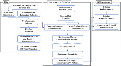
The scope of climate adaptation investment is extended to cover entire land transport networks in TIE. Road and rail screening is performed to omit irrelevant routes out of the target roads and rails using a set of predetermined screening criteria. For instance, responsible entities of transport networks or road and rail locations can be used as criteria. Then, remaining target roads and rails are later classified based on their importance. If additional countermeasures are included, their unit costs should be estimated. Countermeasures are categorized according to their functions. Lastly, a matrix is developed separately for roads and rails by multiplying the unit costs of categorized countermeasures with the total distances of the target roads and rails. The matrix facilitates recommendations for a climate adaptation investment in the transportation sector corresponding to the size of budget and significance of roads and rails. Uncertainty analysis can be done before proceeding to next steps if variations of inputs, e.g., unit costs of countermeasures and total target distance, change the order of magnitude of investments. Then, stakeholders are consulted to determine applicable combinations of countermeasures for target roads and rails. Finally, investments are summed up to achieve a total investment on climate adaptation.

The I&FF assessment is separated into two components: investment flow (IF) and financial flow (FF) (UNDP, 2020b). Here, an investment flow refers to the capital cost of a new physical asset with a life of more than one year. A financial flow refers to continuous spending on programmatic measures that include expenditures other than those for expansion or installation of new assets. All of these can only be started once an increment in total investment is calculated. Total investment represents the difference between the baseline and adaptation scenarios. Investments in the typical annual construction and restoration of roads and rails are considered in the baseline scenario. Operation and maintenance of ongoing infrastructure, as well as other activities to enable or promote usage of infrastructure, should also be covered under the baseline scenario. Such analyses are challenging for most developing countries because data are scattered over different entities and generally provided in terms of overall investments, rather than the actual expenses in a particular sector. Estimations for the total investment in the adaptation scenario are much simpler compared to those for the baseline scenario. Total investments in the adaptation scenario are achieved by adding total costs of applying selected countermeasures on selected target roads and rails to total investments in the baseline scenario. Annual investments for both scenarios are calculated to determine investments and financial flows. A time frame can be set up corresponding to emission reduction goals prescribed by the national determined contribution (NDC). To develop investment and financial flows for the adaptation scenarios, investments and associated costs of selected countermeasures will be added to general expenditures in the baseline scenario.

3. Thailand case study

This case study covers only climate adaptation investment in the land transportation sector. Both CBA and I&FF assessment were conducted considering the climate and geographical conditions of Thailand.

3.2. Cost–benefit analysis

3.2.1. Identification of study areas

The process of picking up the route is done in consultation with the Department of Highways (DOH), Thailand. Highway 3196 (km 2+100 - 2+700) was selected as the target route as it goes along the irrigation canal and has been heavily affected by repeated floods. The railway system in Thailand is divided into inter-city railways and city railways. The current study focuses on the inter-city railways which are under the State Railways of Thailand (SRT). SRT Northern Line was selected as the target line for the case study. Only the section from km 485 to km 642 is selected as the study area since, based on the discussion with SRT, it experienced flash floods in the past.

3.2.2. Net present value and benefit–cost ratio estimation

The initial investment is achieved as a result of applying a mixture of countermeasures on the selected sites. As a result, all combinations that include mechanically stabilized earth wall yield negative NPV (B/C ratio < 1) because its initial investment is quite high compared to other countermeasures. On the other hand, NPV for cape seal treatment is positive even if it is combined with laying the road surface higher. A more detailed consideration of the benefits is needed before implementing all these countermeasures. As for rails, all NPVs and B/C ratios indicate that all countermeasures are not feasible from a business perspective. However, the analyses should take indirect benefits into consideration along with direct benefits.

3.3. Total investment estimation (TIE)

The selection criteria for roads and rails are achieved under this framework. The road criteria are: (i) the road is owned by the Department of Highways (DOH) or the Department of Rural Roads (DRR); and (ii) roads must be located near a canal or a river. There are two items for rail screening: (i) the railway line is adjacent to a mountain; or (ii) the railway runs perpendicular to a river or a waterway. The whole country’s road and rail network is narrowed down to only the most vulnerable to floods using the proposed criteria. Then, the remaining roads and railways are further categorized according to their usage and traffic capacity. The classification of roads is divided into three tiers: (i) single-digit and two-digit national highways; (ii) three-digit national highways; and (iii) four-digit national highways and all rural roads. However, rail routes are only divided into two tiers: total number of passenger-kilometres more than 1 billion and less than 1 billion.

The selected countermeasures done in the CBA were categorized in order to develop the target–countermeasure cost matrix. The countermeasures were categorized into three groups, namely flood management, flood avoidance and structure reinforcement. A matrix was developed by matching the categorized countermeasures with the classified roads and rails. This matrix is accomplished with several assumptions; for instance, the unit costs of each countermeasure are estimated based on past experience and some countermeasures are only applied to 5% of the total distance of the selected roads and rails based on consultations with the experts.

3.4. Investment and financial flow assessment

The study site of I&FF assessment is extended from the CBA study of isolated assets to the whole transportation sector in Thailand. As stated in the methodology, baseline scenarios can be determined by first identifying relevant institutions. DOH, DRR and SRT are responsible for government transport investment. The baseline scenario is determined considering available data for projects funded by government, under public private partnerships (PPP) or through foreign loans or aid. To simplify assessments of baseline scenarios, investments and cashflows of the past five years are gathered and averaged, then the average value is used to project remaining annual investments throughout the timeframe using gross domestic product (GDP) growth to discount to year 2022. The total investment in the adaptation scenario was estimated using the target–countermeasure cost matrix developed in TIE.

As the total investment in adaptation scenarios is very large for the responsible entities, the case study needs to further consider investments and financial flows. The investment flow (IF), financial flow (FF) and operation and maintenance (O&M) costs were estimated and added to general expenditures in the baseline scenario. The timeframe was set to 2022–2030, which corresponds to the carbon neutrality pledge at COP26 (Ministry of Foreign Affairs, 2021).

4. Conclusion

This study proposes total investment estimation (TIE) and demonstrates its capability to link CBA and I&FF assessment using the case studies of Thailand’s land transport sector. The results from TIE can serve as input data to calculate investment and financial flows. It was found that the target-countermeasure cost matrix can facilitate selection of appropriate climate-proofing countermeasures for the target roads and rails by providing a big picture of the investment over a long time. Furthermore, it can be used to tailor climate adaptation investments corresponding to the size of budget and significance of the roads and rails. As such, TIE smoothed out the transition from CBA to I&FF assessment by filling in the missing link. The proposed TIE will be beneficial to those conducting CBA and would extend from a particular site to cover an entire sector of a country.

Acknowledgments

The authors would like to express their sincere gratitude to the United Nations Development Programme (UNDP) for its financial support through the UNDP Thailand/ NDC Support Project, ‘Delivering Sustainability Through Climate Finance Actions in Thailand’.

Disclosure statement

The DRI Technical Conference 2022 was sponsored by CDRI, along with editorial work of the Conference Proceedings. However, CDRI did not influence the research, data, findings, and views presented in the research papers.

Cost–benefit analysis of NbS using flood resilient scenario modelling (FReSMo)CONTACT Aishwarya Narendr [email protected]

ABSTRACT

Coastal flood impact assessment on built infrastructure is critical for coastal resilience and sustainability, but the estimation process is rather complex. Especially for developing countries that have limited access to information regarding future flood extent, land use change and damage behaviour of elements at flood risk such as residential buildings. The rising impact of coastal floods on built infrastructure requires an economical and lucrative intervention that is impracticable without the estimation of the potential damage cost. Therefore, the proposed flood resilient scenario modelling (FReSMo) aims to estimate the probable cost of future damage that could be further used in determining the efficacy of IPCC defined nature-based solutions (NbS) in reducing flood impact on built infrastructure in Sagar Island, West Bengal. FReSMo is made up of a multivariate damage model that is developed to have a flexible application over spatial (local to regional) and temporal (flood character and intensity) dimensions. The future built-up area for 2050 is predicted using a patch-growing algorithm FUTURES model that generates realistic outcomes based on landscape metrics, temporal land use growth, demographic and socio-economic characteristics. The return period of high-water flooding is calculated using peak over threshold (PoT) analysis of long-term tidal data. The flood extent is mapped using a connected bathtub model derived from the Cartosat DEM. Residential building damage against a 100-yr flood event is calculated using FReSMo in pre- and post-mitigation scenarios. The cost–benefit analysis shows that an investment in mangroves will reduce the impact of floods by 70–75%, with a total benefit of about 261.3% for a 48-hr flood and 254.6% for a 24-hr flood.

Keywords:

• Coastal flood impact
• damage assessment
• multivariate damage model
• nature-based solutions

1. Introduction

The global flood situation is likely to deteriorate with climate change as a catalyst for high water anomalies, sea level rise and tidal surges (Kirezci et al., 2020). Tropical location, the relative difference from the mean sea level and unregulated change in land cover affect the frequency, intensity and spatial extent of cyclone and high-tide-induced floods, causing prolonged inundation of low-lying coastal areas.

Loss of built infrastructure is a prominent impact of prolonged inundation, adversely affecting coastal wellbeing. Due to the floods caused by three recent cyclones – Bulbul (2019), Aamphan (2020) and Yaas (2021) – India has recorded losses of 0.28, 2.86 and 0.3 million houses respectively in the affected districts of West Bengal (District Disaster Management Department (DDMD), 2020; UNICEF, 2021). Despite the damage, coastal areas continue to thrive, establishing the dominance of economic and physiographic factors in controlling growth potential over flood-exposed regions (Dhiman, VishnuRadhan & Eldho, 2019). Hence, there is immediate need for strategies for the reduction of the impact of coastal flooding on built infrastructure.

Investing in flood resilient strategies requires evaluations of the damage cost to built infrastructure made of vernacular-style mud housing, which is a popular low-cost building typology prevalent across the coastal villages in India (PMAY-G, 2016). Damage estimation requires the empirical observation of how buildings behave in floods, something that is usually not available in the developing regions. Moreover, the evidence available on the behaviours of mud buildings does not justify the holistic nature of slow-rising coastal flood scenarios that include both depth and duration impacts, requiring a multivariate approach.

In addition, the ‘proximity induced vulnerability’ associated with coastal floods highlights the relevance of ‘spatial level’ interventions as resilient strategies to curb future flood impacts (Balica, Wright & Van der Meulen, 2012). The presence of high-resolution spatial datasets and precisely selected built-up growth parameters are indispensable for generating realistic assessments of future flood susceptibility.

Therefore, the proposed FReSMo (flood resilient scenario modelling) integrates flood exposure, building damage behaviour and land use analysis from a spatial-dynamic perspective to estimate the probable loss of built-up areas in the year 2050 for a 100-yr flood event. The loss estimated in the pre-and post-mitigation scenario is analysed using cost–benefit analysis to determine the effectiveness of the flood resilience strategy, such as the IPCC-defined NbS, in reducing the damage cost to buildings.

2. Study area

The West Bengal coastline in India is exceptionally sensitive to the high-water anomalies due to relative sea level rise (RSLR), recorded at about 5.16 mm in Diamond Harbour, way above the national average (Das, 2021). The state also inhabits maximum densely populated rural settlements below the 10 m low elevation coastal zone (Columbia University, 2007). Further, the gradually sloping continental shelf, the volatile character of the Bay of Bengal, unregulated change in land cover and the dearth of effective climate change action plans for infrastructure protection in rural coastal communities necessitate immediate intervention.

Sagar Island, with an area of 282 km² and located at the southern tip of the state, is entirely rural, with a population of about 0.2 million (Figure 1). The Sagar block and its 47 villages are repeatedly affected by coastal water intrusion due to tidal anomalies and storm surges. It is the nearest refuge for the displaced population from adjacent parts of the drowning Sundarbans estuary, emphasizing the need for flood resilience intervention.

Figure 1. Study area: Sagar Island.

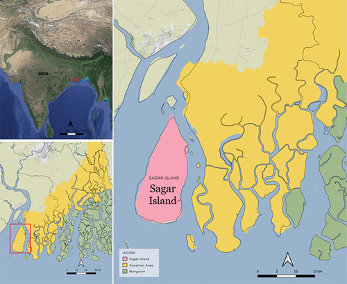
3. Data and method

Development of cost–benefit analysis flood resilient intervention using FReSMo is summarized in four step : Multivariate-probabilistic damage model; FUTURES model for built-up prediction; Spatial extent of flood exposure; Cost -benefit analysis of NbS using FReSMo. Table 1 presents the list of the secondary dataset used in the research.

Table 1. Datasets and their description.

Data Type	Content	Usage	Source
Remote sensing data	LISS IV (2012, 2014, 2018 & 2020) Spatial resolution 5.6 m	Present map, Predicted land use	National Remote Sensing Centre (NRSC)
	Stereo pair of Cartosat Spatial resolution 2.5 m	Digital devation model (DEM), Slope, Coastal flood modelling
	Spatial distribution of buildings, socio-economic, infrastructure and accessibility growth seeds	Land use map, Predicted land use, Exposure analysis of coastal floods	Google Earth, Open Street Maps, Bhuvan (India)
Hydrological data	Daily records of high water and low water (1980–2022)	High Water Line (HWL), Return period analysis	Kolkata Port Trust, West Bengal, India
Census data	Administrative boundary	Present and predicted land use map	Goverment of West Bengal, Census of India (2011)
	Village-wise population data (1991, 2001 & 2011)	Land use prediction, Land demand calculation	District census handbook for 24 South Paraganas, Census of India (2011)

Table 2. Description of parameters used for built-up area prediction.

Sl No.	Parameters	Category	Description
1	Land use, land cover	Physiographic	Temporal change in land use landcover determines the upcoming growth in the region, as people tend to settle in communities
2	Slope	Physiographic	The communities tend to crop up in valley regions or gentler slopes rather than on the peaks.
3	Mangroves	Physiographic	The mangroves are protected regions as they act as a natural buffer to cyclonic storms
4	Distance from a tidal creek	Accessibility/ economic	Source of economic activity such as fishing, crab farming and prawn farming
5	Distance from the amenities	Accessibility/ economic/socio-demographic	Amenities here are schools, religious places, banks, bus stops, docks, hospitals and a police station
6	Distance from the shoreline	Accessibility/ economic	Shorelines are a source of attraction due to the facility for trade and commerce
7	Distance from the road	Accessibility/ economic	Distance to roads aids regional development by enhancing connectivity to educational, health care and business activities.
8	Population and exponential projection of population for 2050	Socio-demographic	The population size is used to estimate the residential land demand in coming years based on the area of current housing. The exponential increase is best suited for the Indian subcontinent based on its past trend analysis

Table 1. Datasets and their description.

Data Type	Content	Usage	Source
Remote sensing data	LISS IV (2012, 2014, 2018 & 2020) Spatial resolution 5.6 m	Present map, Predicted land use	National Remote Sensing Centre (NRSC)
	Stereo pair of Cartosat Spatial resolution 2.5 m	Digital devation model (DEM), Slope, Coastal flood modelling
	Spatial distribution of buildings, socio-economic, infrastructure and accessibility growth seeds	Land use map, Predicted land use, Exposure analysis of coastal floods	Google Earth, Open Street Maps, Bhuvan (India)
Hydrological data	Daily records of high water and low water (1980–2022)	High Water Line (HWL), Return period analysis	Kolkata Port Trust, West Bengal, India
Census data	Administrative boundary	Present and predicted land use map	Goverment of West Bengal, Census of India (2011)
	Village-wise population data (1991, 2001 & 2011)	Land use prediction, Land demand calculation	District census handbook for 24 South Paraganas, Census of India (2011)

3.1. Multivariate-probabilistic damage model

A multivariate damage model adopts an experimental approach to describe the cumulative behaviour of flood depth and duration (using Equation 1)(1) $Damage\hspace{0.17em}ratio\hspace{0.17em}\left(a\right)=\hspace{0.17em}f\left(depth,\hspace{0.17em}duration\right)$(1) on the traditional housing of Sagar Island. A series of structural tests performed to analyse the flood resistance of mud wall samples post-inundation resulted in the generation of damage/ loss ratios shown in Figure 2. The damage ratio is suggestive of the repair costs of components (from Equation 2)(2) $\mathrm{E}\mathrm{q}DC=\sum _{i=1}^{n}a\cdot C{C}_i$(2) . The repair cost values were obtained as per the West Bengal schedule of rates. The study adopts the damage behaviour of the dominant material (mud walls from Figure 2 in this case) to estimate the damage of cost to the entire building.

(1) $Damage\hspace{0.17em}ratio\hspace{0.17em}\left(a\right)=\hspace{0.17em}f\left(depth,\hspace{0.17em}duration\right)$(1)

(2) $\mathrm{E}\mathrm{q}DC=\sum _{i=1}^{n}a\cdot C{C}_i$(2)

Where DC is the damage cost of the entire building, CC = cost of an individual component, n = number of components in the building, and a = loss ratio of the component.

Figure 2. Damage matrix based on experiment for Sagar Island.

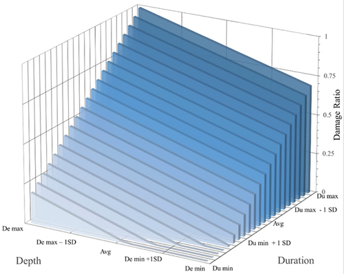
3.2. FUTURES model for built-up area prediction

A patch-growing algorithm-based FUTURES model is used to simulate growth of built-up areas within Sagar Island. The simulation is based on three modules that work together: (i) Suitability module; (ii) Demand module; and (iii) PGA module (Lopez-Farias, Valdez & Garcia-Robledo, 2021). The first module looks at the effects of growth parameters described in Table 2 to figure out how likely it is for a non-built-up pixel to be transformed into an area to transform into a built-up area. The growth parameters considered for the analysis were categorized into physiographic, socio-demographic, economic infrastructure and accessibility. The temporal land use map for 2012, 2014, 2018 and 2020 were extracted based on standard methods using the Gaussian maximum likelihood classifier (Aithal, SHivamurthy & Ramachandra, 2017; Narendr et al., 2022; SHivamurthy & Ramachandra, 2017). The land use was classified as water, agriculture, vegetation, built-up, mangroves and others. In contrast to conventional cellular automata (CA) models, logistic regression was used to rank the parameters, reducing the inherent bias of multi-criteria decision tools.

Table 2. Description of parameters used for built-up area prediction.

Sl No.	Parameters	Category	Description
1	Land use, land cover	Physiographic	Temporal change in land use landcover determines the upcoming growth in the region, as people tend to settle in communities
2	Slope	Physiographic	The communities tend to crop up in valley regions or gentler slopes rather than on the peaks.
3	Mangroves	Physiographic	The mangroves are protected regions as they act as a natural buffer to cyclonic storms
4	Distance from a tidal creek	Accessibility/ economic	Source of economic activity such as fishing, crab farming and prawn farming
5	Distance from the amenities	Accessibility/ economic/socio-demographic	Amenities here are schools, religious places, banks, bus stops, docks, hospitals and a police station
6	Distance from the shoreline	Accessibility/ economic	Shorelines are a source of attraction due to the facility for trade and commerce
7	Distance from the road	Accessibility/ economic	Distance to roads aids regional development by enhancing connectivity to educational, health care and business activities.
8	Population and exponential projection of population for 2050	Socio-demographic	The population size is used to estimate the residential land demand in coming years based on the area of current housing. The exponential increase is best suited for the Indian subcontinent based on its past trend analysis

The second module computes per capita land demand for the predicted population assuming the existing consumption trend. Finally, a PGA module simulates built-up area dynamics based on the suitability, growth parameters and land demand estimations using the inherent features of landscape metrics for a realistic outcome.

3.3. Spatial extent of flood exposure

Coastal floods are associated with tidal water ingress/movement beyond a demarcated high-water line (HWL). The elevation value of the high-water line was determined using a long-term mean of daily high-water records. The flood return period beyond this HWL was analysed applying extreme value theory and peak over threshold. The 100-yr return flood inundation was mapped using a DEM-based connected bathtub model to analyse the built-up susceptibility (Shivamurthy, Narendr & Aithal, 2022).

3.4. Cost–benefit analysis of NbS using FReSMo

The development of NbS (mangroves) in low-lying coastal areas can be considered a workable and pragmatic solution for reducing overall flood risks. Hence, the assessment involves a comprehensive survey of literature to estimate the cost of mangrove development to reduce the emerging costs of damage.

The rationale behind the calculation is in line with Equation 1(1) $Damage\hspace{0.17em}ratio\hspace{0.17em}\left(a\right)=\hspace{0.17em}f\left(depth,\hspace{0.17em}duration\right)$(1) , meaning that a reduction in the flood impact factors (depth and duration) shall aid in an overall reduction of the damage cost of building.

4. Results

4.1. Damage assessment using FReSMo

The impacts of floods on built infrastructure was assessed by combining the development of built-up areas in 2050 with a 100-yr flood return under two duration scenarios of 24 hrs and 48 hrs (Figure 3). The damage stage and probable cost of flood damage can be retrieved for each elevation pixel that varies significantly with inundation period for the mud buildings. The damage statistics presented as pre-mitigation in Figure 4 indicate the total number of buildings likely to be damaged by such an event.

Figure 3. Damage stage analysis of predicted built-up area (2050) in 100-yr flood: return period for (a) 24 hrs and (b) 48 hrs.

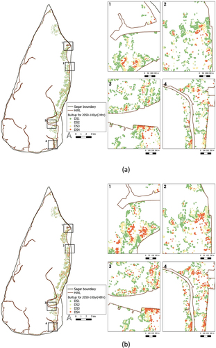
Figure 4. Building damage stage analysis against 100-year flood-return period (a) pre-mitigation, (b) post-mitigation using NBS.

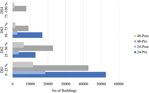
4.2. Cost–benefit analysis

Table 3 summarizes the data necessary to determine the costs and benefits of developing mangrove plantations throughout the high-risk regions of Sagar Island. A 100 m patch of mangroves can subdue flood heights by about 50% (World Bank, 2022). Hence, investment in mangrove plantations will reduce flood damage cost up to 70–75% with a total benefit of 261.3% for a 48-hr flood and 254.6% for a 24-hr flood. The reduction in the number of flood-prone dwelling units is shown in Figure 4 as post-mitigation scenarios.

Table 3. Description of parameters used for estimating cost-benefit of NBS.

Initial flood depth for (100-yr return) (D1)	2.251 m above the HWL
Cost of one building unit (30 m^2) (in Rs)	40,000
Total built-up damage due to D1 (in Rs)	1291.36 million (24 hrs) 1467 million (48 hrs)
New flood depth after NBS (100-yr return) (D2)	1.251 m above the HWL
Total built-up damage due to D2 (in Rs)	335.45 million (24 hrs) 377.19 million (48 hrs)
Per area cost of plantation (in Rs)	Rs 30.81 million per sq. km
Area of plantation required for Sagar Island	0.945 km^2
The total cost of plantation	Rs 29.11 million
Total benefit	254.6%–261.3%

5. Conclusion

The research applied FReSMo to analyse the benefits of NbS in reducing the impact of coastal floods on built infrastructure. The FReSMo is made up of an experimentally derived multivariate damage matrix, which is integrated with the 100-yr flood exposure and built-up area prediction for 2050 to estimate the probable cost of damage. The probable cost of damage is re-evaluated in a post-mitigation scenario where mangroves were used as a spatial level flood resilient strategy. The results signify a 70–75% decrease in the damage cost.

The analysis provides a high-resolution approach for flood damage estimation with limitations such as the use of the Census 2011 for population prediction, considering it the most authentic data source available, and the presence of epistemic uncertainty with the use of a single building archetype for the analysis. The study presented the analysis for mud buildings, but it can be extended to other typologies through a similar procedure. Moreover, the rationale behind using FReSMo for analysing NbS is helpful for informed decision-making.

Acknowledgments

We are thankful to IIT Kharagpur, the Kolkata Port Trust, the NRSC and the Government of West Bengal for extending their data and financial support for the research. We also thank Ms Praneta Nadupalli of RCGSIDM, IIT Kharagpur, for her dedication and help in the process of research work.

Disclosure statement

The DRI Technical Conference 2022 was sponsored by CDRI, along with editorial work of the Conference Proceedings. However, CDRI did not influence the research, data, findings, and views presented in the research papers. .

Multi-hazard risk assessment of critical coastal infrastructure in the Eastern Economic Corridor of ThailandCONTACT Indrajit Pal [email protected]

ABSTRACT

Asian countries are facing multiple hazards with higher frequency and intensity. These disasters are damaging to infrastructure and disrupting services. Probability of hazards and their impacts on these critical infrastructures becomes important in order to safeguard the normal functioning of society. The Eastern Economic Corridor (EEC) is a special investment zone in the coastal areas of the Chonburi, Rayong and Chachoengsao provinces of Thailand. This research attempts risk assessment of critical infrastructure with a focus on the transport, health and education sectors in relation to floods, cyclones and coastal erosion in the EEC. Identification of key indicators for hazard, exposure, sensitivity and capacity for composite risk assessment of critical infrastructure was the primary consideration for the multi-hazard context. The result shows that districts with a very high risk level are Si Racha (Chonburi) and Ban Chang (Rayong) and associated critical infrastructures. A moderate level of risk is found in Klaeng (Rayong), while Ko Sichang (Chonburi) and Sattahip (Chonburi) are considered low risk. With this knowledge, Laem Chabang Port and U-Tapao Airport are in very high-risk zones, whereas Map Taphut Port, situated in Muang Rayong, has a high level of risk. Further, available risk information provides an opportunity for efficient allocation and prioritization of resources for risk mitigation measures.

KEYWORDS:

• Critical infrastructure
• coastal infrastructure
• risk assessment
• eastern economic corridor
• Thailand

1. Introduction

Thailand is a centre of economic growth in the Southeast Asian region. The country’s economic growth is propelled by export-oriented manufacturing supported by robust infrastructure development (UKABC, 2019). That infrastructure is also prone to natural hazards such as cyclones, floods, storm surges and tsunamis. During the Thailand flood of 2011, damages and losses were to the tune of US$46.5 billion dollars across various sectors (Haraguchi & Lall, 2015).

Recently, natural hazards have been more frequent and intense in Asian countries, and especially in Thailand (European Commission, 2019). These disasters have been causing damage to infrastructure, including critical services. As a result, it is crucial to understand the current hazard situation and its potential impact on these critical infrastructures. Critical infrastructure is defined as assets and services that offer essentials related to the physical structures that enable the economy and society to function (Marcelo et al., 2020). Inaccessibility to critical infrastructure increases pressure on people’s health, quality of life, education, employment and economics. Even though definitions and categorizations of critical infrastructure differ across countries, their role is important for running societies and the economy, as well as the population’s safety and well-being (Mohanty, Chatterjee & Shaw, 2020).

It is important to identify the risks to critical infrastructure and address them to build long-term resilience in infrastructure systems. This study aims to assess current situations of hazards in coastal areas in Thailand with a focus on the Eastern Economic Corridor (EEC) located in the provinces of Chonburi and Rayong. Establishing risk maps is essential for determining the amount of risk to critical coastal infrastructure and informing the path of investment direction.

2. Methodological framework

1.1. Objectives of the study

This research aims to review hazard profiles, critical coastal infrastructure and the risk index in the coastal areas/regions of Chonburi and Rayong provinces, Thailand. The research is further divided into two sub-objectives:

1. To evaluate the hazard profiles in coastal areas of Chonburi and Rayong provinces.

2. To assess risks to critical infrastructure from different hazards in the coastal areas.

1.2. Study area

The EEC consists of three provinces: Chachoengsao, Chonburi and Rayong. This research covers coastal areas where critical infrastructure concentrations are exposed to multi-hazards. There are eight districts along the coastal area in the provinces: Muang Chon Buri, Si Racha, Ko Sichang, Bang Lamung and Sattahip in Chonburi; and BanChang, Muang Rayong and Klaeng in Rayong. The total coastline of Chonburi (130 kilometres) and Rayong (95 kilometres) is 225 kilometres (Figure 1).

Figure 1. Study area map.

Source: Authors.

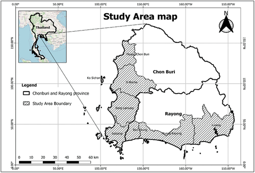
1.3. Methods and analysis

Multi-hazard risk assessment of coastal critical infrastructure involves identification of hazards, exposure, vulnerability and other risk parameters. The steps involve hazard assessment, which focuses on multi-hazards with the highest potential impact on EEC, such as flooding, cyclones and coastal erosion. A risk index is calculated by integrating/combining an exposure index, a sensitivity index and an adaptive capacity index to identify existing critical infrastructure and determine the EEC’s risk exposure level.

The study employs a relative risk assessment rather than an absolute risk assessment method for critical infrastructure risk calculation. It compares the composite risk of districts within the study area. Further, risk is the product of hazard and vulnerability, and inversely related to coping capacity, where vulnerability comprises exposure and sensitivity (Rana & Routray, 2016). The following formulas are used in this study:

$R_i=H_i\times V_i$

R_i = Risk index

H_i = Hazard index

V_i = Vulnerability index

Each indicator is analysed and standardized according to its contribution to hazard and vulnerability. The indicators were weighted and normalized neutral to obtain the multi-hazard risk index map. In order to do that, a vulnerability assessment of coastal critical infrastructure was considered further. The following vulnerability formula is used:

$V_i=\frac{E{x}_i\times S_i}{A{C}_i\hspace{0.17em}}$

V_i = Vulnerability index

Ex_i = Exposure index

S_i = Sensitivity index

AC_i = Adaptive capacity index

The formula used to calculate the vulnerability of critical coastal infrastructure was adopted from IPCC (2014) and U.S. National Parks (Tormey, Peek & Young, 2016). According to the procedure normalized value formula, a normalization strategy with weighting/weightage was used (Mullick, Tanim & Islam, 2019). Figure 2 shows the detailed methodological framework adopted for this study.

Figure 2. Methodological framework of the study.

Source: Authors.

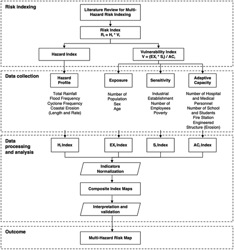
1.4. Selection of indicators and data

The dataset was selected through a comprehensive literature review involving secondary quantitative data from reliable sources within Thai government departments, census statistics and climate data. As shown in Table 1, indicators for the hazard component include flood hazard, cyclone hazard and coastal erosion hazard.

Table 1. Risk assessment indicators and variables.

Risk Components	Indicators	Variables	Description and Justification	Scale	Data Source	Reference
Hazard	Flood Hazard	Total rainfall	Higher amount of rainfall has a greater possibility of the hazard	mm	Meteorological Department, Ministry of Information and Communication Technology	Mandal and Choudhury (2014); Ali et al. (2019); Ghosh and Mistri (2021)
		Number of flood occurrences	It depicts the greater possibility of flood hazard	Number	Department of Disaster Prevention and Management, Chonburi and Rayong office	Rana and Routray (2016)
	Cyclone Hazard	Number of cyclone occurrences	The recorded number of cyclone occurrences by district depicts the greater possibility of cyclone hazard	Number	Department of Disaster Prevention and Management, Chonburi and Rayong office	Hoque et al. (2019)
	Coastal Erosion Hazard	The ratio of coastal erosion by length	The recorded coastal erosion in Chonburi and Rayong over decades	District ratio	Department of Marine and Coastal Resources	Hoque et al. (2019)
		The ratio of coastal erosion by area	The recorded coastal erosion in Chonburi and Rayong over decades by area	District ratio	Department of Marine and Coastal Resources	Hoque et al. (2019)
Exposure	Demography	Population	Refers to the number of people living within a specific unit of measurement	Person	Department of Provincial Administration, Ministry of Interior	Ali et al. (2019); Das et al. (2020)
		Sex	Male and female refer to the ratio of number of men and women in the area	Person	Department of Provincial Administration, Ministry of Interior	Rufat et al. (2015); Das et al. (2020)
		Age group	Children aged < 18 years old and senior citizens aged 19–100 years old	Person	Department of Provincial Administration, Ministry of Interior	Rufat et al. (2015); Sahana and Sajjad (2019)
Sensitivity	Economic	Employment	Number of employees	Person	Chonburi and Rayong Provincial Industrial Office	Qasim et al. (2017)
Industrial establishment	Number of established industries in the area			Place	Chonburi and Rayong Provincial Industrial Office	Qasim et al. (2017)
Adaptive Capacity	Hospital and health centre	Number of hospitals and health centres	Refers to the capability to reduce loss and mortality of climatic hazards	Place	Chonburi and Rayong Provincial Health Office	Yoo et al. (2010); Das et al. (2020)
		Number of medical personnel	The ability to support a large number of patients; the higher number of medical personnel, the higher number of thorough care to patients	Person	Chonburi and Rayong Provincial Health Office	Yoo et al. (2010); Das et al. (2020)
	Education	Number of students	Refers to accessibility of education in the area	Person (student/total population by district)	Educational Service, Chonburi and Rayong Provincial Office of Local Administration	Fekete (2012)
	Fire Stations	Number of fire stations	Refers to capability to respond to emergency incidents	Place	Department of Disaster Prevention and Management, Chonburi and Rayong office	Speakman (2008); Yu et al. (2020)
	Engineered structures for coastal erosion	Number of construction lengths	The more coverage of constructing engineered structures protecting coastal erosion	Length	Department of Marine and Coastal Resources	Noor and Abdul Maulud (2022)

2. Results and discussion

This study covers three main hazards of floods, cyclones and coastal erosion as having maximum impacts on the functionality and performance of critical infrastructure.

2.1. Multi-hazards in EEC

A composite multi-hazard risk index is developed using a proposed hazard index. It was found that Mueang Rayong and Kleang were the districts with the highest risk due to their high exposure to floods, storms and coastal erosion, while Si Racha, Mueang Chonburi and Baan Chang are in the lower risk zone. Details of these indices are given in Table 2 and a multi-hazard map developed based on these indices is depicted in Figure 3.

Figure 3. Multi-hazard map of Chonburi and Rayong province.

Source: Project team.

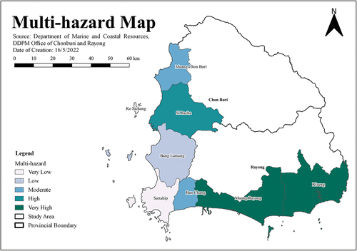
Table 2. Multi-hazard index.

Province	District	Normalized Erosion Rate	Normalized Erosion Length	Normalized Cyclone Occurrence	Rainfall Normalized	Normalized Flood Occurrence	Hazard Index
Chonburi	Mueang Chon Buri	0.40	0.14	0.07	0.87	0.18	0.33
	Bang Lamung District	1.00	0.13	0.07	0.39	0.00	0.32
	Si Racha District	1.00	0.15	1.00	0.33	0.27	0.55
	Ko Sichang District	0.00	0.00	0.00	0.41	0.00	0.08
	Sattahip District	1.00	0.05	0.14	0.00	0.09	0.26
Rayong	Mueang Rayong	0.34	1.00	0.71	1.00	1.00	0.81
	Ban Chang	0.31	0.17	0.71	1.00	0.27	0.49
	Klaeng	0.33	0.34	0.71	1.00	1.00	0.68

Source: Project team.

2.2. Risk index

The risk index is determined by two components, namely hazard index and vulnerability index, which are represented in Table 3, by the risk formula mentioned in the methodology section.

Table 3. Risk index of case study districts.

Province	District	Hazard Index	Vulnerability Index (Ex * S/AC)	Risk Index (H * V)
Chonburi	Mueang Chon Buri	0.33	0.66	0.22
	Bang Lamung District	0.32	0.23	0.07
	Si Racha District	0.55	1.16	0.64
	Ko Sichang District	0.08	0.00	0.00
	Sattahip District	0.26	0.07	0.02
Rayong	Mueang Rayong	0.81	0.48	0.39
	Ban Chang	0.49	1.05	0.52
	Klaeng	0.68	0.14	0.10

Source: Project team.

2.3. Multi-hazard risk index

A multi-hazard risk map (Figure 4) presents the total risk of districts in Chonburi and Rayong provinces to multi-hazards. Si Racha (Chonburi) and Ban Chang (Rayong) are at highest risk, whereas Muang Rayong (Rayong) is at high risk and Muang Chonburi and Klaeng (Rayong) are at moderate risk, respectively.

Figure 4. Multi-hazard risk map.

Source: Project team.

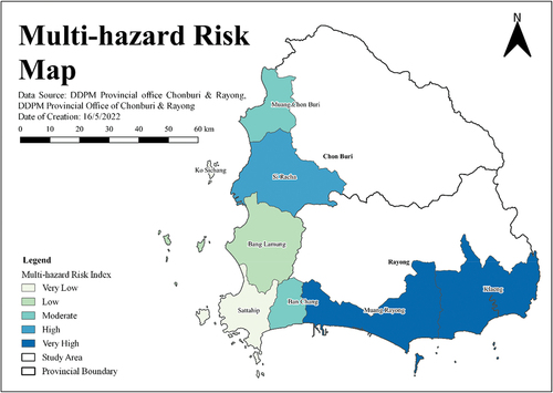
2.4. Multi-hazard and critical coastal infrastructure risk

Map Ta Phut Port and Laem Chabang Port are situated at ‘very high’ and ‘high’ risk levels, respectively. Similarly, U-Tapao Airport is operated at a ‘very high’ risk level. Some of the districts in Chonburi and Rayong along the coastline show a relatively low number of hospitals and health centres. For instance, Ban Chang and Muang Rayong have a low number of hospitals and health centres, compared to other districts, especially Klaeng. This leads to the difficulty of access to healthcare services for locals. However, the catchment area or service radius should be considered in order to reflect the current situation appropriately.

Figure 5. Multi-hazard risk and critical coastal infrastructure map.

Source: Project team.

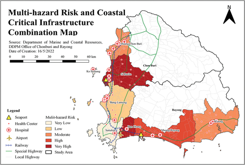
3. Conclusion

Multi-hazard risk assessment is a powerful tool for identifying the highest risk areas and districts with the highest potential for disaster losses. In this study, Si Racha and Ban Chang fall under the highest risk zones. Being an industrial province, it has major exposure due to high population density. However, with the similar hazard potential of the mainland, Ko Sichang island has a low risk because of its low population density, which leads to low exposure. Similarly, Klaeng has a low vulnerability as a big city in Rayong, but the district itself has less exposure in terms of population, age, sex and hazards, but high adaptive capacity. This research can be used as a starting point for detailed area-specific risk assessment. By identifying high-risk and low-risk districts, a more efficient and effective resource allocation for districts can be made. Critical infrastructure needs to be built with better quality and resilience in districts where high risk is present. Likewise, the adaptive capacity can be improved in these districts as well. Furthermore, the Thai government has the policy to invest and set up an EEC project in Chonburi and Rayong, and acknowledging risks to the coastal areas is crucial.

Acknowledgments

This paper is an outcome of the research carried out as part of the Coalition of Disaster Resilient Infrastructure (CDRI) Fellowship Programme (Application No. 210117487) awarded to the Asian Institute of Technology, Thailand for the period May 2021 to June 2022.

Disclosure statement

The DRI Technical Conference 2022 was sponsored by CDRI, along with editorial work of the Conference Proceedings. However, CDRI did not influence the research, data, findings, and views presented in the research papers.

Exploring the potential of urban open spaces as city flood mitigation infrastructureCONTACT PC Nivya [email protected] Karmakar [email protected]

linkedin.com/in/nivya-pc-048a4713b

linkedin.com/in/shreya-karmakar-she-her-bb26ab142

[email protected], linkedin.com/in/sharon-maria-sajan-992350228

ABSTRACT

Public spaces are city dwellers’ open-air living rooms and define cities’ cultural, social, economic and political functions. They are of three types: streets and pedestrian access; open and green spaces, such as parks, plazas, water bodies and waterfronts; and public facilities, such as libraries, community centres and markets. With a growing urban population, cities’ land and other vital natural resources are becoming constrained, causing pollution, congestion, deficit of essential services, housing scarcity, slum settlements, encroachment and increased vulnerability to disaster risks. This growing constraint has also resulted in urban flooding in many cities due to a significant reduction in areas for infiltration and the water detention that manages stormwater run-off. Climate change and increasing extreme events further exacerbate the risk of urban flooding. Due to high land values in urban areas, building stormwater detention infrastructures to control urban floods is capital intensive with low returns on such investments. Many cities like Rotterdam, Tokyo, Copenhagen and others have diversified open spaces for recreational purposes and urban flood mitigation. Blue-green surface solutions with reduced piping infrastructure have shown potential to be more effective and economic than piped solutions. This paper explores innovative solutions adapted by various cities across the world for making cities resilient to flooding. The focus of the paper is more on existing cost- and time-effective hybrid solutions in cities that combine grey, blue and green infrastructure for flood risk reduction.

KEYWORDS:

• Urban flooding
• resilience
• open spaces
• detention
• stormwater

1. Introduction

Urban areas depend on intricate and interrelated systems of critical infrastructure services which are often hampered by disasters. Extreme and changing weather patterns, natural hazards and disasters brought on by anthropogenic activities are straining people and impacting the prosperity of cities (IPCC, 2022). Many cities lack sufficient drainage systems, solid waste management and water resource management, which leads to floods and health issues. Wetland reclamations and land encroachments due to increased urbanization have threatened the ability of city ecosystems to ensure flood regulation and protection (Alikhani, Nummi & Ojala, 2021). Realizing the need to preserve these critical natural assets within the urban landscape, China launched its ‘sponge cities’ programme to retrofit natural landscapes in 30 pilot cities that would have the ability to absorb 70% of the stormwater run-off by 2030 (Zevenbergen, Fu & Pathirana, 2018).

Urban flooding is an accumulation of precipitation in a built-up environment, particularly in a highly populated area, when the drainage system exceeds its capacity to handle the run-off (Wikipedia, n.d.). Urban flooding damages private and public properties and has a significant detrimental influence on the urban economy. Critical services that get suspended have a cascading impact on other interdependent services. The cost of restoring and rebuilding houses and public infrastructure puts a strain on the funds of municipal corporations. Such experiences underline the need for resilience and paradigm shifts in urban governance. Resilience and catastrophe risk reduction must be incorporated in urban design and master plans/strategies to achieve sustainable development (UNISDR, 2012).

Most cities emphasize mitigation measures to strengthen their resilience to floods and other disasters. The measures range from hard infrastructure solutions like building detention tanks, tunnels and reservoirs, to soft adaptation measures like restricting land use and implementing policies. Establishing strong linkages between a city’s climate change adaptation strategies and its long-term resilience-building is critical for developing city action plans in an ever-evolving urban setting. Nature-based solutions (NbS) are some of the cost-effective solutions that are gaining more popularity. One of the reasons for this paradigm shift towards NbS is the cost associated with hard infrastructure solutions. In cities, land is one of the major constrained resources. Acquiring urban land for building massive flood prevention infrastructure like stormwater tunnels and tanks is not an economically feasible solution. Even though flood prevention infrastructure has the benefit of reducing the losses due to disasters, there are no direct economic returns from the investment. Due to urban land scarcity, many cities like Tokyo, Chicago and Hong Kong have adapted underground detention basins and tunnels, but doing so requires heavy machinery and technology for underground drilling and construction.

The world population in cities today stands at about 55% and is predicted to be 70% by 2050. Asia and Africa will contribute to almost 90% of this urbanization surge (UN DESA, 2018). More urbanization is expected from low-income and developing economies in coming years and investments in cost-intensive flood mitigation infrastructures for flood mitigation in cities will be difficult to afford for the cities in these countries. So, a cost-effective solution requiring less land is needed for making cities flood resilient.

Public spaces are the areas that are openly accessible and are of three types: streets and pedestrian access; open and green spaces, such as parks, plazas, water bodies and waterfronts; and public facilities, such as libraries, community centres and markets (UN Habitat, 2016). Open spaces in cities are the citizens’ living rooms and they provide socio-economic and health benefits to the city dwellers which are often undervalued (UN Habitat, 2020). Many cities have diversified urban open spaces for flood prevention, and it is very cost-effective compared to the hard infrastructure solutions. Rotterdam, Copenhagen, Tokyo and Newcastle have explored the multifunctionality of open spaces and used them for flood prevention. This paper discusses some existing cost- and time-effective hybrid solutions in these cities, which combine grey-blue and green infrastructure for flood risk reduction.

2. Case studies

2.1. Case 1: water plaza in Rotterdam

The water plazas in Rotterdam are urban open spaces that are used to collect rainwater during rainy seasons and are used for recreational purposes during dry weather. They provide additional water storage facilities in densely built-up areas. The plazas get filled up only during heavy rains and the water flows to the plaza through a sewer and pump system. During light and medium showers, water is pumped away from the streets and is discharged to sewers, washing away the dust in the streets. As the intensity of the rain increases, the pressure in the pump to process water also increases, allowing excess water to flow to the plazas instead of to the sewers. The water, which is clean as the initial flush with dirt has been discharged to sewers, is again passed through a purifying filter before being discharged to the plaza. Once the heavy rain is over and water levels are back to normal, the plaza will be emptied by opening the pipe that is connected at the lowest point and it will be discharged to moats (Bravo, 2013). Benthemplein in Rotterdam is one of the water plazas developed by Rotterdam City Council to manage stormwater run-off from heavy rainfall. Benthemplein has three pools that get filled up during heavy rains. The central pool is the largest and deepest pool, which turns into a water well during heavy rains; when empty it is used as a football or basketball court.

Figure 1. Water Square/Plaza in Benthemplein.

Source: ‘File:Benthemplein terrain skate gestion eau.jpg’ by Cathrotterdam and ‘Rotterdam Wasserplatz Benthemplein’ by stadtlandschaft from creative commons.

2.2. Case 2: detention boulevard in Copenhagen

Sønder Boulevard is a road with a fenced median strip of grass situated in Copenhagen, the capital city of Denmark, and is the longest gathering and recreational space in the city. There are many bars, restaurants and co-working spaces along the green space. During dry weather the boulevard is an active recreational area; during the rainy season, stormwater infiltrates through the green area in the median and the run-off on the road is reduced. Under heavy rains or cloudbursts, the amount of water will be high, and the green strip converts to a stream to carry excess run-off. Once the rain is over, the green strip is back for recreational purposes (Ramboll, 2013).

Figure 2. Sønder Boulevard.

Source: a) Author; b) ‘Sønder Boulevard’ by Tony Webster from creative commons; c) ‘Sønder Boulevard 4/4’ by Lars K. Jensen from creative commons.

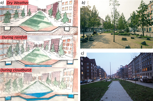
2.3. Case 3: Grand Mall Park in Tokyo, Japan

Grand Mall Park in Tokyo was developed under the Minato Mirai (MM21) project to increase disaster resilience and environmental sustainability in the city. The project was completed in 1989 and later renovated in 2015. A concept of vertical water circulation for stormwater management was introduced in the design during renovation. The park has a site area of 23,000 m² and is surrounded by commercial buildings, museums and retail businesses. A pedestrian axis of 25 m connects the waterfront to the station. Tall zelkova trees and sea-wave patterned furniture cover the landscape of the park. The level of pavers and macadam beneath pavements are the major components of vertical water circulation. Below the pervious pavements, a 700 m stormwater storage macadam is provided, retaining stormwater that infiltrates through gutters, pervious pavements and planting beds. This stormwater macadam allows the tree roots to penetrate, unlike the normal pavement layers that restrict vegetation growth. The water retention capacity of the macadam in Grand Mall Park is 76 L/m³ and the macadam is made of crushed stones mixed with humous for a higher water retention capacity (Jha, Lamond & Bloch, 2012). The stormwater that is being stored in the pavement macadam is absorbed by the trees and other vegetation in the park. This reduces the surface run-off and thereby flooding. Also, it gives a cooling effect and creates a microclimate in the area, which increases the usability of the open spaces.

Figure 3. Grand Mall Park.

Source: Left: Author; Right: KennethYR from creative commons.

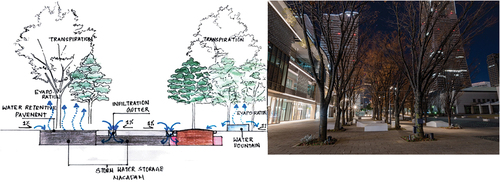
2.4. Case study 4: retention basins and ponds in Newcastle

Newcastle, situated on the north-western bank of the River Tyne in north-east England, is a planned, compact city. The Greenfield site towards its northern and western parts, open land that has never been built on, has traditionally been protected from large residential and commercial development due to the variety of environmental risks the area faces. However, with the growth in population and demand for housing, Greenfield has seen arbitrary construction activities over the years that have significantly hampered the region’s ecological heritage and stormwater drainage.

Since 2012, Newcastle has experienced a spate of fluvial flooding events, following which the Newcastle City Council has started reclaiming the Greenfield site by investing in BGI (blue-green infrastructure) to improve the city’s stormwater management mechanism. One of the exemplary interventions among these have been sustainable drainage system (SuDS) ponds. The SuDS management train is a concept used for SuDS and is shown in Figure 4. The management train starts with prevention at source, i.e., management of rainwater where it falls and then management at larger downstream sites and regions. The SuDS ponds are designed to collect stormwater through roof gutters, downpipes and road gullies, and divert it to a combined sewer network (O’Donnell et al., 2017). The city has created attenuation basins covered by an amphitheatre that allows safe and contained storage of excess surface run-off, and making it a recreational space during non-flood conditions. Similarly, attenuation basins are created on the flood plains near rivers. During tidal surges, when the floodplains get filled, water is forced from the river into the attenuation basins for detention (Morgan & Fenner, 2017). This reduces peak flows in the downstream sewer and surface water drainage systems. When the peak flow in the river settles, water is discharged into the river or combined sewage system through a flow control channel at a controlled, predevelopment rate.

Figure 4. SuDS management train.

Source: Author.

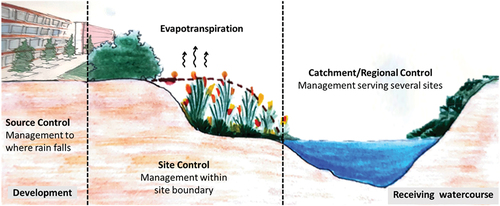
3. Lessons learnt

In many cities urban open spaces are designed only for recreational purposes, whereas they have other functionalities, and can be used as an option for enhancing flood resilience in cities. The cases discussed in this paper exhibit open spaces having a significant impact on the urban landscape, improving the presence of vegetation and delivering health advantages. On the other hand, they lower peak stormwater run-off, the amount of water going to drains and improve run-off water quality. Using public open spaces for flood mitigation helps in reducing land acquisition costs, thus lowering capital investment and making it a cost-effective solution. In addition, multi-purpose sustainable drainage systems can also help restore habitats, biodiversity and places for recreation with vital ecosystem services for settlers. BGI solutions in open spaces, such as water plazas and permeable attenuation basins, offer a riparian buffer to surface water run-off and improve the developed landscapes’ stormwater management capabilities, lowering vulnerability to extreme flooding events. Though these solutions do not make the city completely resilient to floods, they reduce flood risks with less effort, funds and time compared to other hard infrastructure methods, which require longer commissioning time. These BGI solutions in open space planning are more investment-friendly than piped solutions and create diverse direct and indirect benefits for the socio-economic conditions of a city.

4. Conclusion

In normal weather conditions, urban infrastructure often remains unrecognized in the background, serving only primary functions such as recreation. The cases reviewed in this paper exemplify the advantages of designing urban spaces for many purposes. Both hard and soft adaptation methods are required for enhancing adaptation and building resilience within urban landscapes. The cases demonstrate that cost-effective BGI solutions can contribute to a landscape’s resilience and adaptive capability to flooding by reducing flooding risks. However, challenges in implementation limit their uptake and innovation for other landscapes. BGI can be included in urban open spaces through better management of biophysical uncertainties, coordination from all urban stakeholders during design, and exploring co-financing mechanisms to ensure financially sustainable, socially acceptable and technically sound solutions. The potential of open spaces to act as flood-resilient infrastructure should be advocated as a nature-based, cost-effective and time-efficient solution for flood resilience in cities.

Disclosure statement

The DRI Technical Conference 2022 was sponsored by CDRI, along with editorial work of the Conference Proceedings. However, CDRI did not influence the research, data, findings, and views presented in the research papers.

Potential of Himalayan wetlands for mountain disaster risk reduction under climate changeCONTACT Santosh Subhash Palmate [email protected]

ABSTRACT

Mountain glaciers are retreating almost everywhere in the world, including the Himalayas, due to melting under temperature increase and climate change. Disasters like floods and landslides become uncertain and severe in the Himalayas, which could cause property damage, life devastation and biodiversity disturbances. Himalayan wetlands that support mountain ecosystem services are also vulnerable to climate change. It is likely that with a warming climate, new natural wetlands may develop that can change the risk of mountain disasters by acting as natural resilient infrastructure. This study aimed to estimate the probability of new wetlands and their potential role in disaster risk reduction. A maximum entropy algorithm was used to model the impact of climate change on glacier melting, new wetland development and the wetlands’ potential for reducing disaster risks. Spatial data for topographic characteristics, land properties and bioclimate variables were used as model inputs. Existing wetland locations in India were considered for training and testing the model. Results showed that the vulnerability of the Himalayan wetland would continue as the temperature increases and extreme precipitation events are likely to happen. High-altitude glacier melting can probably develop new wetlands in depressed mountain areas. It will increase the water holding and soil deposition potential of the Himalayan wetlands.

KEYWORDS:

• Mountain disasters
• climate change
• resilient infrastructure
• natural wetlands
• transboundary himalaya

1. Introduction

As temperature increases cause global warming, mountain glaciers are retreating almost everywhere in the world (Laghari, 2013; Sharma et al., 2022). Moreover, due to climatic change, major mountain disasters like floods and landslides become uncertain and happen frequently, potentially causing socio-economic losses and ecological biodiversity disturbances (Gupta et al., 2019; Hoy et al., 2016).

Among mountains, the Himalayan system consists of over 50 peaks higher than 7000 m. The Himalayan region faces sudden and calamitous disasters, like floods and landslides, due to climatic events and anthropogenic activities (Laghari, 2013). This causes the uncertain availability of Himalayan water sources, including mountain wetlands, for sustaining ecosystem services (O’Neill, 2019; Palomo, 2017). Himalayan wetlands (lakes and ponds, meadows, marshes, swamps, bogs and fens) are generally fed by precipitation, snowmelt water, glacier meltwater or permafrost melt. Studies have revealed that the Himalayan wetlands are affected by climatic changes and anthropogenic activities (Gupta et al., 2019; Palomo, 2017). Such wetlands are important for reducing flooding effects and minimizing landslides by depositing soil, lowering surface water flow rates, storing water and maintaining ecosystem services (Rashid & Aneaus, 2020). The role of wetlands in strengthening resiliency to mountain disaster risks and their changes over time is crucial to understand for managing the Himalayan mountain systems (Haeberli & Drenkhan, 2022; Hoy et al., 2016).

The Himalayas are the most influenced natural system under uncertain climatic events, such as cloud bursting and heavy rainfall. This causes occurrences of sudden flash floods and landslides in different altitude regions of the Himalayas (Akhtar, Ahmad & Booij, 2008). Furthermore, as climate change increases, temperature rises can hasten Himalayan glacier melting in the sensitive high-altitude region, resulting in less glacier coverage over time (Gupta et al., 2019; Laghari, 2013; Sharma et al., 2022). Melted glacier water flows along slopes of mountain landscapes and forms wetlands in depressed mountain areas by accumulating water, soil and sediment flows (Sharma et al., 2022). Preparing an inventory of such wetlands is difficult and time-consuming in the mountain region, which leads to limited wetland information. Also, the sensitive international boundaries of the Himalayas are another major issue that restricts the availability of ground observed data. Open-source remote sensing data can be an alternative solution for conducting research on the Himalayan wetlands (Rashid & Aneaus, 2020).

This research aims to assess the potential of current and future Himalayan wetlands in reducing mountain disaster risks with a focus on floods and landslides. The study has been planned with the objectives: (i) to prepare an inventory of existing and predict the probability of new mountain wetland formation due to high-altitude glacier melting; and (ii) to study the potential role of these wetlands for reducing disaster risks in the Himalayan mountains under different climate change scenarios.

2. Study area

This study has focused on the transboundary Himalayan mountain systems of Asia. The Himalayas are spread over several nations, including India, Pakistan, Afghanistan, Nepal, Bhutan, Myanmar and China (Figure 1). After the Arctic and Antarctica, the Himalayan Mountains cover the third largest deposit of ice, snow and glaciers in the world. The Himalayas have the largest glacier, Siachen, and other notable glaciers such as Hispur, Baltoro, Nubra and Biafo. Major river systems of Asia, namely the Ganga, Indus, Brahmaputra, Yarlung, Yellow, Mekong, Nuijang and Tangtze, also originate from the Himalayas (Phartiyal, Singh & Nag, 2018).

Figure 1. Location and elevation maps of the transboundary Himalayan mountain region in Asia includes the world’s 10 highest peaks.

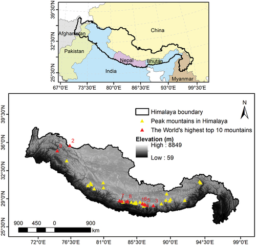
3. Data and methods

3.1. Data collection and processing

In this study, digital elevation model (DEM) data was obtained from the United States Geological Survey (USGS) Earth Explorer website, land cover data from the NASA Earth Data website, and bio-climate data from the WorldClim website. The wetlands’ location data was obtained from the Indian government reports and the Indian Space Research Organisation (ISRO) wetland atlas website of India (Table 1).

Table 1. List of data and their source websites.

Data	Website link
DEM	https://earthexplorer.usgs.gov/
Land cover	https://urs.earthdata.nasa.gov/
Bioclimate variables	https://www.worldclim.org/data/bioclim.html
Indian wetlands point location data	https://vedas.sac.gov.in/en/National_Wetland_Inventory_and_Assessment_(NWIA)_Atlas.html
MaxEnt model	https://biodiversityinformatics.amnh.org/open_source/maxent/

The global CMIP6 climate model (BCC-CSM2-MR) dataset has been used to extract precipitation and temperature data-based bio-climate variables. Shared Socioeconomic Pathways (SSP) of CMIP6 data, at the lowest level (ssp126) and highest level (ssp585), were used in the study to understand the minimum and maximum levels of climate change impact in the Himalayas. Also, the analysis was performed for short-term (2021–2040) and long-term (2081–2100) periods to check the difference between ongoing and future climate change impacts. Hence, a total of four types of climate scenario combinations – (i) ssp126_2021-2040, (ii) ssp126_2081-2100, (iii) ssp585_2021-2040 and (iv) ssp585_2081-2100 – have been used in the study for future wetland inventory modelling.

Required datasets of land characteristics, topographic features and bio-climatic properties were processed and generated in the ArcGIS software environment. Land and topographic variables, namely landforms, the Normalized Difference Vegetation Index (NDVI), the Normalized Difference Water Index (NDWI), the Normalized Difference Snow Index (NDSI) and bioclimatic variables, namely isothermality, temperature seasonality, mean temperature of driest quarter, precipitation of driest month, and precipitation of coldest quarter, were used (Figure 2). Wetland location (point) data, a total of 849 wetlands with an area >10 ha, were used to train and test the model prediction (Figure 3). The model training was performed with 60% and testing with 40% of the wetland point location data.

Figure 2. Spatial maps generated using open-source datasets for the modelling.

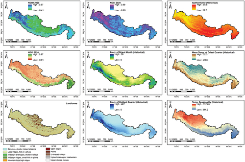
Figure 3. Wetland location sampling used for training and testing of the model.

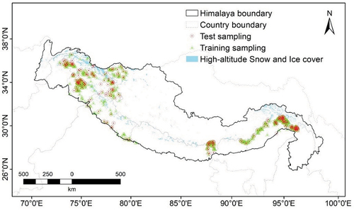
3.2. Maximum entropy (MaxEnt) model

This study uses a maximum entropy (MaxEnt) algorithm to model the existing geographic distribution of Himalayan wetlands using specific point location data. The MaxEnt model (Table 1) helps lower the modelling uncertainties and affirm wetland inventory simulation (O’Neill, 2019). It iteratively computes the probability of distribution of a response that maximizes entropy, i.e., closest to a uniform probability of wetland occurrence, based on sensitive inputs such as topographic features, land characteristics and climate variation (O’Neill, 2019). All the model inputs were prepared in a specific format employing interactive time-series data processing. In this study, the MaxEnt is used for both historical and future wetland inventory modelling, as the impact of climate change accelerates glacier melting and forms natural wetlands in the mountains.

4. Results and discussion

4.1. Model performance evaluation

Model simulation performance was evaluated using a threshold independent measure and the area under the curve (AUC). It helps quantify the model’s capability of correctly simulating a random occurrence locality of wetland. In this study, an AUC of 0.950 for training and an AUC of 0.943 for testing shows an acceptable model performance (Figure 4).

Figure 4. Performance evaluation of the model.

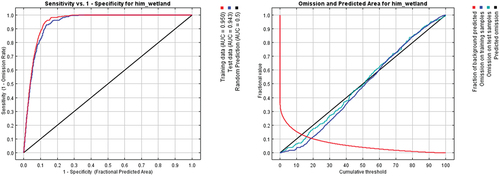
4.2. Himalayan wetland inventory

4.2.1. Historical inventory modelling

The climate data over 1970–2000 was used for historical inventory modelling. Probabilities of the occurrence of wetlands in the whole Himalaya region are grouped into five categories (Figure 5). High to very high probability classes 0.6–0.8 and 0.8–1.0 were considered to analyse wetland areas. The high probability class covers about 1,04,660 sq km (i.e., 5.5%), and the very high probability class covers about 38,018 sq km (i.e., 2%) of the total wetland probability area. Further, the glacier class from land cover data of the year 2019 was used to extract wetland probability distribution in the high-altitude Himalayan region. In the high and very high probability classes, the total historical wetland area is only about 0.8%. This area can contribute to lowering water flows and minimizing soil erosion in mountain landscapes.

Figure 5. Himalayan wetland inventory using historical climate data.

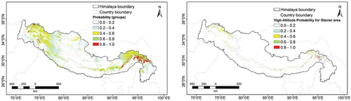
4.2.2. Future inventory modelling

During analysis, only precipitation and temperature data-based climate variables were changed in the model. Results of the future wetland inventory modelling show a significant variation of wetland distribution in the future due to climate change impacts (Figure 6). The highest probability of wetland formation in the future is in the eastern and western Himalayan regions. The high probability class (0.6–0.8) covers 9.2% to 17.3%, and the very high probability class (0.8–1.0) covers 11.9% to 12.9% of the total wetland probability area in the Himalayas. Hence, in the future, the wetland area will increase, which can support strengthening mountain disaster resilience in the transboundary region. On the other hand, there are chances of issues like restrictions to accessing tourist areas, mountain routes, and other places because of new wetland development, which provides scope for future research in mountain regions (Haeberli & Drenkhan, 2022). The probability of such a new wetland development was evaluated for the Sikkim mountain region (O’Neill, 2019). Recently, wetlands have been found to be protection infrastructure from climate-related hazards for coastal areas of Italy (Ivčević et al., 2021), and they can also help in disaster risk reduction based on published scientific evidence (Sudmeier-Rieux et al., 2021).

Figure 6. Himalayan wetland inventory based on different future climate scenarios.

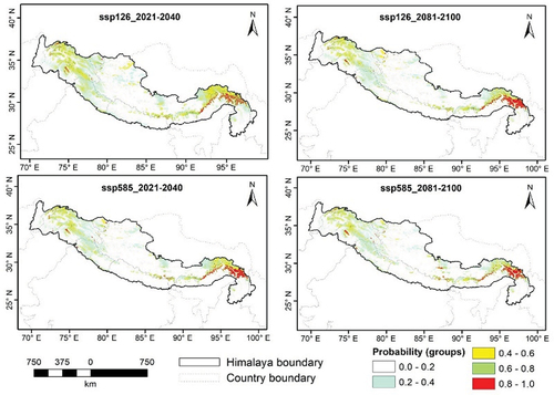
4.3. Limitations of the research

Disaster risk in the mountain region is controlled by only climatic changes related to precipitation and temperature, enabling climate-data-based predictions. However, in reality, anthropogenic activities somehow induce the propagation of mountain disasters, adaptation strategies and their impacts on human life (Hoy et al., 2016). But, this study covers only climate change impacts and excludes anthropogenic impacts. For future inventory modelling, selected topographic variables were kept constant. Significant change in such topographic variables would not be possible naturally in the mountain region unless there were rapid anthropogenic activities. Furthermore, this research is limited without on-field social surveys, which could provide human insights and perceptions about Himalayan glacier dynamics and formations. Also, the data related to floods and landslides are not readily available to cross-check which locations tend to be prone to mountain disasters. This would help recognize probable wetland areas that can reduce future disaster impacts, as well as restrict access to mountain tourist places and routes.

5. Conclusions

The study uses open-source datasets of remote sensing,historical and future bioclimate variables to understand the effects of climate change due to new wetlands likely to be developed in the Himalayan Mountains. A maximum entropy algorithm was used to assess the climate change impacts on Himalayan glacier melting, new wetland development, and the potential of probable wetlands in reducing/increasing disaster risks in the mountain region. The model simulated probability ranges from 0.6–0.8 and 0.8–1.0 were mainly utilized to assess the new wetland development. The study leads to the following conclusions:

1. Wetland dynamics, in terms of their numbers and area/capacity, can alter the mountain disaster impact by increasing the water holding capacity and soil deposition potential over time.

2. Due to the high sensitivity of wetlands to short- and long-term climate change, the Himalayan wetlands are more vulnerable in the low-altitude (<3000 m) as well as high-altitude (>3000 m) regions.

3. The study revealed that the mountain wetlands could act as a natural resilience infrastructure to climate-based disasters.

4. Results in the form of transboundary wetland datasets, probable wetland maps and an overview of the wetlands’ potential in the future could help local stakeholders and policymakers to manage mountain floods and landslides and sustain the wetland ecosystem functions.

Overall, this study improves our understanding of the impact of high-altitude transboundary glacier melting on new wetland formation, as well as their potential to reduce disaster risks. The proposed methodology is novel and can be used for future wetland inventories, and extendable to other mountain/transboundary regions, where wetland functions are primarily driven and controlled by glacier melting. Also, this study has provided cross-institutional research and information-sharing opportunities and facilitated knowledge synthesis for transboundary stakeholders.

Acknowledgments

We sincerely acknowledge the Coalition for Disaster Resilient Infrastructure (CDRI) for providing a research grant under the CDRI Fellowship Progamme (Application ID 210115447), as well as the Texas A&M AgriLife Research, Texas A&M University (TAMU) for providing necessary lab facilities for research. We are thankful to the CDRI Technical Expert Group (TEG) member Dr Rama Umesh Pandey, Associate Professor & Head, School of Planning and Architecture, Bhopal, India, and Dr Parisa Kloss, Executive Director of Resilient Urban Planning and Development (RUPD) GbR, Bonn, Germany for providing constructive suggestions and motivation.

Disclosure statement

The DRI Technical Conference 2022 was sponsored by CDRI, along with editorial work of the Conference Proceedings. However, CDRI did not influence the research, data, findings, and views presented in the research papers.

Inclusion of people with disabilities in disaster and climate risk reduction planning: a case from Bhubaneswar, OdishaCONTACT Prasanna Bhangdia [email protected] Murhekar [email protected]

ABSTRACT

India has a vast topography and changing climatic conditions, which makes it prone to a myriad of disasters. Planning ahead for a vulnerable area can help to prevent catastrophic losses. But the way society responds to such situations varies from person to person. People with disabilities are the ones who are exposed to the highest risks and need special attention while planning disaster response policies. Research suggests that the mortality rate amongst people with disabilities tends to be two to four times higher than the remaining population, highlighting their high vulnerability. Hence this research aims to address this global issue by developing an inclusive, context-specific digital tool at a city level to integrate all strata of differently abled and elderly populations for effective disaster and climate risk reduction infrastructure planning. The city of Bhubaneswar, the capital of Odisha state, is selected for the case study. Based on risk and vulnerability assessments of cyclonic hazards, a digital tool is proposed with a dashboard for decision-makers and a mobile application for citizens. A mobile application helps to identify location and type of disability, as well as show efficient ways to exit and reach nearby shelter. It also has a feedback mechanism to provide inputs for policy planning. This research demonstrates that such interventions can improve the quality, efficiency and sustainability of disability-inclusive disaster risk reduction strategies in a city, and also help build a disaster-resilient inclusive society.

KEYWORDS:

• Disability inclusion
• disaster risk reduction
• climate resilience

1. Introduction

The impact of a disaster on a society varies from person to person. Persons with disabilities face severe problems on account of their exposure to such events, a shortage of available infrastructure, inappropriate facilities, lower self-confidence and lower general socio-economic conditions (DiDRR, 2021). Research shows that the mortality rate amongst persons with disabilities tends to be two to four times higher than the rest of the population. In such a situation it becomes important to consider this section of the society in preparing disaster relief plans.

As per reports by the World Health Organization (WHO) and the World Bank, more than one billion people around the world have some disability issues. In India, about 2.1% of the population have some sort of disability. But this number is not exact since there is a lack of comprehensive, desegregated and up-to-date data on persons with disabilities. This is directly related to the Sendai Framework priority 1 and Sustainable Development Goals (SDG) 2030, ‘Leave No One Behind’, which demands more granular data to establish evidence-based policy.

A few researchers have reported that while preparing city specific or state specific disaster relief policies, the opinions of persons with disabilities are not considered. This calls for representation, coordination and partnership with organizations of persons with disabilities in preparing Disaster Risk Reduction. Another crucial factor identified from the literature is the lack of accessibility that persons with disabilities face. For example, while designing disaster shelters the structural safety of buildings NDMA (2019) is given priority, but fails to integrate universal accessibility.

With all these identified issues, this research advances with an idea of developing a digital tool which will enable local authorities to:

1. Track the locations of persons with disabilities and elderly people in a city.

2. Identify the most suitable evacuation pathways from such locations to the nearest shelters.

3. Monitor safe evacuations of persons with disabilities during times of crisis.

4. Ensure the accessibility of these people to all infrastructure at rescue shelters.

5. Get opinions from all strata of people, including persons with disabilities, while deciding types and quality of rescue shelters, their locations and the requirements of this group during disasters.

2. Objectives

• To assess the study area profile for physical and social vulnerability and carry out the risk assessment for a cyclone hazard.

• To design and develop a digital platform for governance to achieve informed decision-making while planning disability inclusive disaster risk reduction strategies.

• To prepare a digital application for citizens, especially persons with a disability, to get them involved in all stages of disaster risk reduction planning.

3. Methodology

Figure 1. Methodology of the study.

Figure 1. Illustrates the methodology of the study.

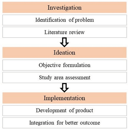
4. Scope and limitations

• This research will produce a dashboard for governance and a mobile application for citizens to achieve informed decision-making for disability inclusive disaster risk planning at city level.

• The mobile application is designed so that it need not be used during the time of the disaster; instead it will be used only pre and post occurrence of the disaster.

• Digital literacy may impact the grassroots penetration of the application proposed in this study.

5. Study area assessment

5.1. About the city

Bhubaneswar, the capital of Odisha state, is situated on the eastern ghats, about 40 km west of the Bay of Bengal coast, at an average elevation of 45 m above mean sea level in Khordha district. Figure 2 shows the location of Bhubaneswar, which has a tropical climate.

Figure 2. Distribution of structural losses corresponding to a 100-year return period for a cyclonic wind hazard.

Source: S. Gupta (2014)

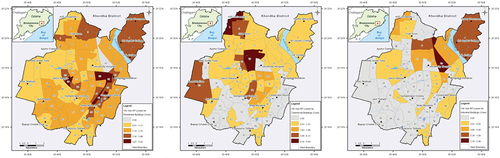
Figure 3. Snippets of the mobile application to be used in the post-disaster scenario for rescue, relief and recovery.

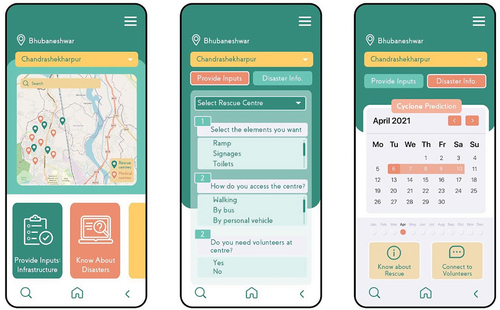
The geo-climatic conditions of Odisha make it vulnerable to various natural hazards (SDMP, 2017), and likewise for the case of Bhubaneswar. Every two years the city faces hazards like cyclones, high winds, floods, heavy rains, drought, heat waves, pest attacks and many more. Hence it is important to understand the characteristics of hazards, as well as their impacts on the city, and identify ways to minimize their negative impacts.

5.2. Physical vulnerability

The type of building and its structure plays an important role in disaster resilience. As per the 2021 census, good residences make up 60% of the city, liveable residences 35% and dilapidated residences 5%. The 40% of dwellings which are not good are more prone to cyclone hazards and other disasters. Of these dwellings, about 5% and 8% are mud buildings and masonry buildings, respectively. Another 10% of buildings have mortar joints but temporary roofs. Around 72% of buildings are built with reinforced concrete cement (RCC) and brick infill, and 4% of buildings with RCC and steel. These statistics show that around 24% of buildings are more prone to damages due to cyclone hazards on account of their structural conditions and type of building material used.

5.3. Social vulnerability

As per the 2011 census, about 9.7% of the population is below six years of age while 9.5% is above 60 years of age, higher than the state’s average. The female population in the city is about 47% while scheduled castes and scheduled tribes constitute about 8% and 5% of total population respectively. These factors especially need to be considered when planning for any disaster resilience activity, along with the physical vulnerability.

5.4. Risk assessment

As per the report of the United Nations Development Programme (UNDP) on hazard risk and vulnerability assessment for Bhubaneswar city, Figure 2 shows the distribution of structural losses (PML) corresponding to a 100-year return period cyclonic wind hazard scenario event for buildings in Bhubaneswar. The total estimated losses for residential, commercial and industrial buildings are about 1108.16, 556.48 and 59.73 INR in millions. The same report claims that losses for transport, utility networks and other essential facilities will be around 69.16, 140.1 and 62.193 INR in millions, respectively.

6. Product

As per the disaster management cycle, the digital tools are intended to prepare for a disaster before the event occurs, as well as prepare for rescue and recovery for a post-disaster scenario. Target users for the mobile application are individuals, volunteers and civil organizations, whereas the intended users of the dashboard are the urban local body.

6.1. Mobile application

6.1.1. Pre-disaster

In pre-disaster scenarios, the application entails informing citizens about rescue shelters available in the city based on their GPS location (Figure 3). After selecting a zone that citizens reside in, the citizens can view the location of rescue shelters and health-care centres that are accessible by them.

The application has a module for citizens to give their inputs regarding the universal accessibility of rescue shelters and to participate in the process of designing infrastructure. Upon clicking the button to ‘provide inputs: infrastructure’, a detailed form appears on the screen with set of questions designed to understand the needs of citizens from the rescue shelter perspective. The form includes questions regarding the design elements that they require for ease of access, amenities for survival, volunteers for help and support in varied tasks. Differently abled and elderly citizens can give their inputs and preferences to make infrastructure inclusive and robust. Volunteers can also assist in collecting inputs for the system, so that even citizens with no access to digital resources could have their voices heard.

The application also includes a component for providing information and training modules to citizens. Information regarding the likelihood of the occurrence of disasters and their frequencies will be displayed as a calendar with details of relocation before an event starts. Furthermore, information regarding rescue and relief operations is also mentioned, including the safest escape route that individuals can take based on their GPS location, as well as routes leading to health-care centres and rescue shelters in case of an emergency. Citizens can also sign up as volunteers on the application and provide community assistance.

Figure 3: Snippets of the mobile application to be used in the pre-disaster scenario for providing inputs, gathering information and training

6.1.2. Post-disaster

After a disaster strikes, citizens can access information regarding escape routes, actions to be taken in case of an emergency, avail themselves of medical care, and request volunteers for any assistance, based on their GPS location (Figure 4).

Escape routes are planned as per the GPS locations of a device and the locations of rescue shelters. Inputs from disaster management units about areas affected by cyclones, flooded areas, road blockages and so on are configured in identifying the safest and fastest routes to a rescue shelter from the location of a citizen’s device. The map navigates a citizen and provides an estimated time for reaching a rescue shelter.

For availing themselves of any medical care, the features in the app provide a map of health-care centres within a 2 km radius from the point of enquiry based on a GPS location. Additionally, the application also provides a volunteer service with a multitude of options to choose from, such as volunteers for medical care, assistance, reporting damage, requesting medication and so on.

Figure 4. Snippets of the mobile application to be used in the post-disaster scenario for rescue, relief and recovery.

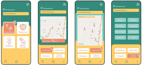
6.2. Dashboard

The second part of the digital product is a dashboard with a real time web-based data visualization portal for decision-making by local authorities. The operations can be classified into the monitoring of weather conditions such as wind speeds to forecast occurrences of disasters and areas that would be affected based on vulnerability assessments, as well as monitoring the rescue and relief operations, deploying the volunteers based on the requests and requirements, and so on.

6.2.1. Pre-disaster

The dashboard integrates the mobile application and the city’s existing early warning system by sending citizens alerts on disasters, disaster prone areas and preparations. Additionally, the application loops back to a database of the dashboard, and collects inputs from citizens for the inclusive infrastructure design, as well as for understanding the requirements of citizens, especially of vulnerable, differently abled and elderly populations.

6.2.2. Post-disaster

The dashboard is linked to the mobile application and provides alerts and information to the citizens regarding the areas affected, road blockages and so on in the recovery stage, as well as aids with the rescue and volunteer requests received on the dashboard warehouse, put forth by the citizens (Figure 5).

Figure 5. Snippet of the data visualization dashboard for informed decision-making.

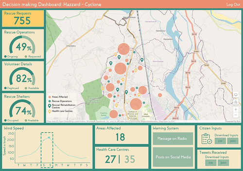
7. How to use this product

The dashboard as mentioned earlier is envisioned to visualize the on-the-ground scenario for the preparation and recovery stages of disaster management, while the mobile application for citizens is an assisting guide for rescue, recovery and inclusion in the decision-making process for inclusive infrastructure.

The tool may act as a digital version of a more robust and inclusive standard operating procedure for disaster management.

To operationalize the digital tool, institutional capacities with trained personnel and civil society organisations, technical capacities with data integration, data storage and application development, are required. Additionally, the constraints of digital divide, data authentication and data privacy are also certain issues to be addressed.

8. Significance of product

8.1. Novelty

This proposal is one of the first of its kind in the Indian context which addresses the disability inclusive DRR at city level by involving all the stakeholders at all stages of decision-making. It covers persons with disabilities to get their valuable input for the inclusive design of infrastructure.

8.2. Feasibility

The process of data input does not require special skills apart from a basic knowledge of mobile use. This product does not require the installation of any separate software systems since it can be plugged into the city’s existing mobile applications and the dashboard of the disaster management department of municipal corporations.

8.3. Scalability

In addition to cyclones, the digital tool can adopt other features to cover other hazards scenarios like heat waves and epidemics, and can ‘Best Suite’ the city specific requirements.

8.4. Impact

The dashboard so developed will help to address the issue of disability inclusion in the formation of DRR at the city level. The digital tool will facilitate actions to resolve governance problems by integrating persons with a disability into decision-making and infrastructure planning.

9. Conclusion

Disaster has negative impacts on all strata of society. Persons with disabilities are most vulnerable to such disasters. The Sustainable Development Goals (SDG) and Sendai Framework prioritize ‘Leaving No One Behind’, which calls for more granular data on disability, without which disaster and climate risks cannot be completely understood by decision-makers.

This research attempted to address this gap by developing an inclusive, context-specific digital tool at the city level to integrate all strata of differently abled and elderly populations for effective planning of disaster and climate risk reduction and infrastructure. Bhubaneswar, the capital city of Odisha, India, was selected as a case study, as it is prone to various disasters with track records of huge losses of life and economic activity. The research uses a risk and vulnerability assessment of cyclone hazards to find measures to include people with disabilities and elderly people in decision-making and disaster planning. The digital tool has a dashboard for governance and a mobile application for citizens. The citizen application helps to collect locations and types of disabilities in the city, based on which the tool identifies safest rescue paths for such people during a crisis. The tool also collects input from persons with disabilities to inform the entire process of DRR planning and maintenance of infrastructure. Such interventions can improve quality, efficiency and sustainability within a disability inclusive and disaster resilient community.

Disclosure statement

The DRI Technical Conference 2022 was sponsored by CDRI, along with editorial work of the Conference Proceedings. However, CDRI did not influence the research, data, findings, and views presented in the research papers.

Notes

1. The sensitivity of a system designs its likelihood to experience particular conditions and the occupancy and livelihood of its characteristics to a given exposure. The adaptive capacity is more focused on adaptability, coping ability, management capacity, stability, robustness, flexibility and resilience (Smit & Wandel, 2006).

1. Classical DCF approaches are the net present value (NPV) rule (invest if NPV>0) and the internal rate of return (IRR) rule (invest if IRR > cost of capital).

2. A useful risk measure should consider whether cash flows are positive (revenues) or negative (expenditures) to estimate certainty equivalents. Risk-averse investors consider risky revenues less valuable and risky expenditures more costly.

3. This is consistent with people’s notions toward risks and willingness to accept smaller revenues or higher costs in exchange for certainty.

4. Its magnitude depends on maturity. In general, risk-free rates increase with longer maturities.

References

- Banerjee, S., & Matsagar, V. A. (2023, May). Earthquake response control of hospital buildings using unbonded fibre-reinforced elastomeric isolators. Sustainable and Resilient Infrastructure, 8;S2: 85–92.
- Bhangdia, P., & Murhekar, A. (2023, May). Inclusion of people with disabilities in disaster and climate risk reduction planning: A case from Bhubaneswar, Odisha. Sustainable and Resilient Infrastructure, 8;S2: 137–142.
- Boothroyd, R. J., Williams, R. D., & Hoey, T. B. (2023, May). ‘InfraRivChange’: A web application to monitor river migration at sites of critical bridge infrastructure in the Philippines. Sustainable and Resilient Infrastructure, 8;S2: 45–51.
- Dahal, K., & Gnyawali, K. (2023, May). Mapping landslide susceptibility and critical infrastructures for spatial decision-making. Sustainable and Resilient Infrastructure, 8;S2: 52–58.
- Dalal, P. H., Wanare, R., Patil, M., Reddy, A. S., Davee, T. N., & Iyer, K. K. R. (2023, May). Water stability test: A tool to assess resilience of geotechnical structures to flooding and water inundation. Sustainable and Resilient Infrastructure, 8;S2: 78–84.
- Espinoza, D. (2023, May). Changing the valuation paradigm to promote adaptive and resilient infrastructure investment: Connecting insurance concepts and valuation. Sustainable and Resilient Infrastructure, 8;S2: 33–37.
- Estrain, A., & Srinivasan, D. (2023, May). An integrated and dynamic approach to assessing risks through capabilities. Sustainable and Resilient Infrastructure, 8;S2: 99–103.
- Gupta, K., & Nikam, V. (2023, May). Flood disaster risk assessment for critical transportation infrastructure under climate change. Sustainable and Resilient Infrastructure, 8;S2: 38–44.
- Nalla, V., Johnson, C. Ranjit, N., Sen, G., Peddibhotla, A., Anand, M. C., … & Bazaz, A. B. (2023). Considering curriculum, content, and delivery for adaptive pathways: higher education and disaster resilient infrastructure in the Indian urban context. Sustainable and Resilient Infrastructure, 8;S1: 143–156.
- Joo, M. R., & Sinha, R. (2023, May). Adaptive pathways for disaster-resilient infrastructure: Resilience assessment as a fundamental requirement. Sustainable and Resilient Infrastructure, 8;S2: 93–98.
- Kamepalli, K. (2023, May). Solar disruptions in space infrastructure. Sustainable and Resilient Infrastructure, 8;S2: 72–77.
- Keam, L., & Harrington, B. (2023, May). Improving resilience outcomes for infrastructure: How to maximize the benefits from disaster and climate risk assessment. Sustainable and Resilient Infrastructure, 8;S2: 20–24.
- Kloss, P., & Samimi, M. (2023, May). Empowering decision-makers to take resilient action towards urban heat island mitigation by developing a multi-dimensional climate model. Sustainable and Resilient Infrastructure, 8;S2: 64–71.
- Nakum, V., Ahamed, M. S., Chatterjee, R., Shaw, R., Isetani, S., & Soma, H. (2023, May). Comprehending school disaster resilience: Deriving indicators for risk-informed school evaluation. Sustainable and Resilient Infrastructure, 8;S2: 59–63.
- Narendr, A., Aithal, B. H., & Das, S. (2023, May). Cost-benefit analysis of NbS using flood resilient scenario modelling (FReSMo). Sustainable and Resilient Infrastructure, 8;S2: 109–114.
- Nivya, P. C., Karmakar, S., & Sajan, S. M. (2023, May). Exploring the potential of urban open spaces as city flood mitigation infrastructure. Sustainable and Resilient Infrastructure, 8;S2: 124–129.
- Pal, I., Kumar, A., Roy, J., Benjachat, N., & Pimpakhun, K. (2023, May). Multi-hazard risk assessment of critical coastal infrastructure in the Eastern Economic Corridor of Thailand. Sustainable and Resilient Infrastructure, 8;S2: 115–123.
- Palmate, S. S., & Kumar, S. (2023, May). Potential of Himalayan wetlands for mountain disaster risk reduction under climate change. Sustainable and Resilient Infrastructure, 8;S2: 130–136.
- Pant, R., Jaramillo, D., & Hall, J. W. (2023, May). Systemic assessment of climate risks and adaptation options for transport networks in East Africa. Sustainable and Resilient Infrastructure, 8;S2: 12–19.
- Parol, J., & Al-Sanad, S. (2023, May). Enhancing infrastructure resilience through structural health monitoring. Presented at DRI Technical Conference 2022.
- Sánchez-Silva, M., & Acuña-Coll, N. (2023, May). Flexible and adaptable strategies for developing sustainable and resilient infrastructure. Sustainable and Resilient Infrastructure, 8;S2: 6–11.
- Vithean, K., Janta, P., Thapmanee, K. Silva, K., & Chollacoop, N. (2023, May). Economic analysis framework for climate adaptation investment in the land transportation sector: A Thai case study. Sustainable and Resilient Infrastructure, 8;S2: 104–108.
- Ziv, N., Soto, D., Sossou, A. E., Philippe, S., Camille, V., & Selouane, K. (2023, May). Resilience performance assessment (RPA): A framework and decision support tool for resilience of infrastructures and territories. Sustainable and Resilient Infrastructure, 8;S2: 25–32.
- Blockley, D., & Godfrey, P. (2017). Doing it differently (2nd) ed.). ICE Publishing.
- Haasnoot, M., Kwakkel, J. H., Walker, W. E., & Ter Maat, J. (2013). Dynamic adaptive policy pathways: A method for crafting robust decisions for a deeply uncertain world. Global Environmental Change, 23(2), 485–498. https://doi.org/10.1016/j.gloenvcha.2012.12.006
- Mizutori, M. (2018). Economic losses and displacement should drive disaster risk reduction efforts. Speaking to the press at the opening of the Asian Ministerial Conference on Disaster Risk Reduction. 3–6 July 2018. © UNISDR.
- Rehak, D., Senovsky, P., Hromada, M., & Lovecek, T. (2019). Complex approach to assessing resilience of critical infrastructure elements. International Journal of Critical Infrastructure Protection, 25, 125–138. https://doi.org/10.1016/j.ijcip.2019.03.003
- Sánchez-Silva, M. (2019). Managing infrastructure systems through changeability. ASCE Journal of Infrastructure Systems, 25(1), 04018040. https://doi.org/10.1061/(ASCE)IS.1943-555X.0000467
- Sánchez-Silva, M., & Calderón-Guevara, W. (2022). Flexibility and adaptability within the context of decision-making in infrastructure management. Structure and Infrastructure Engineering, 18(7), 950–966. https://doi.org/10.1080/15732479.2022.2038642
- Scott, J. (2007, June). System resilience: Capabilities, culture and infrastructure. INCOSE 2007 – 1 Proceedings of the 7th Annual International Symposium, Long Beach.
- Torres-Rincón, S., Bastidas-Arteaga, E., & Sánchez-Silva, M. (2021). A flexibility-based approach for the design and management of floating offshore wind farms. Renewable Energy, 175, 910–925. https://doi.org/10.1016/j.renene.2021.04.121
- AfDB [African Development Bank]. (2014). Study on road infrastructure costs: Analysis of unit costs and cost overruns of road infrastructure projects in Africa.
- Brown, V. (2020). Flooding in East Africa. C40 Cities Finance Facility.
- Erman, A., Tariverdi, M., Obolensky, M., Chen, X., Vincent, R. C., Malgioglio, S., … Yoshida, N. (2019). Wading out the storm: The role of poverty in exposure, vulnerability and resilience to floods in Dar es Salaam. World Bank.
- Global Infrastructure Hub. (2017). Global infrastructure outlook.
- Hallegatte, S., Rentschler, J., & Rozenberg, J. (2019). Lifelines: The resilient infrastructure opportunity. World Bank.
- Horvat, T., Bendix, H., Bobek, V., & Skoko, H. (2021). Impacts of investments in infrastructure projects on emerging markets’ growth: the case of East African countries, Economic Research-Ekonomska Istraživanja, 34:1, DOI: 10.1080/1331677X.2020.1860799
- Kesete, Y., Raffo, V., Pant, R., Koks, E., Paltan, H., Russell, T., & Hall, J. (2021). Climate change risk analysis of Argentina’s land transport network. World Bank.
- Koks, E. E., Rozenberg, J., Zorn, C., Tariverdi, M., Vousdoukas, M., Fraser, S. A., Hall, J. W., & Hallegatte, S. (2019). A global multi-hazard risk analysis of road and railway infrastructure assets. Nature Communications, 10(1), 2677. https://doi.org/10.1038/s41467-019-10442-3
- Makena, B., Osunga, M., Kingori, S., & Abdillahi, H. S. (2021). An application of flood risk analysis for impact based forecasting in Kenya. Kenya Red Cross.
- Njogu, H. W. (2021). Effects of floods on infrastructure users in Kenya. Journal of Flood Risk Management, 14(4), e12746. https://doi.org/10.1111/jfr3.12746
- Oh, J. E., Espinet Alegre, X., Pant, R., Koks, E. E., Russell, T., Schoenmakers, R., & Hall, J. W. (2019). Addressing climate change in transport, vol. 2, Pathway to resilient transport. World Bank.
- Hickford, A. J., Blainey, S. P., Pant, R., Jaramillo, D., Russell, T., Preston, J., Hall, J. W., Young, M. & Glasgow, G. (2023). Decision Support Systems for Resilient Strategic Transport Networks in Low-Income Countries: Final Report. High Volume Transport Applied Research Programme.
- Pant, R., Koks, E. E., Russell, T., & Hall, J. W. (2018a). Transport risks analysis for the United Republic of Tanzania: Systemic vulnerability assessment of multi-modal transport networks. Oxford Infrastructure Analytics Ltd.
- Pant, R., Thacker, S., Hall, J. W., Alderson, D., & Barr, S. (2018b). Critical infrastructure impact assessment due to flood exposure. Journal of Flood Risk Management, 11(1), 22–33. https://doi.org/10.1111/jfr3.12288
- Pearce, D., Atkinson, G., & Mourato, S. (2006). Cost-benefit analysis and the environment: Recent developments. Organisation for Economic Co-operation and Development.
- Schaller, N., Kay, A. L., Lamb, R., Massey, N. R., van Oldenborgh, G. J., Otto, F. E., Sparrow, S. N., Vautard, R., Yiou, P., Ashpole, I., Bowery, A., Crooks, S. M., Haustein, K., Huntingford, C., Ingram, W. J., Jones, R. G., Legg, T., Miller, J., Skeggs, J., … Allen, M. R. (2016). Human influence on climate in the 2014 southern England winter floods and their impacts. Nature Climate Change, 6, 627–634. https://doi.org/10.1038/nclimate2927
- Wang, G., Wang, D., Trenberth, K., Erfanian, A., Yu, M., Bosilovich, M., & Parr, D. (2017). The peak structure and future changes of the relationships between extreme precipitation and temperature. Nature Climate Change, 7(4), 268–274. https://doi.org/10.1038/nclimate3239
- World Bank. (2018). Road costs knowledge system (ROCKS): Doing business update.
- World Resources Institute. (2020). Aqueduct floods hazard maps: https://www.wri.org/data/aqueduct-floods-hazard-maps
- Coalition for Climate Resilient Infrastructure. (2022). Physical climate risk assessment methodology.
- Equator Principles. (2020). EP4 July 2020.
- EU Technical Expert Group on Sustainable Finance. (2020). Taxonomy report technical annex: updated methodology & updated technical screening criteria.
- ICF World Bank Group. (2012). IFC performance standards on environmental and social sustainability.
- IPCC.(2020). The concept of risk in the IPCC sixth assessment report: a summary of cross-Working Group discussions. A. Reisinger et al., Eds.
- IPCC. (2021). Summary for policymakers. In V. Masson-Delmotte, P. Zhai, A. Pirani, S. L. Connors, C. Péan, S. Berger, N. Caud, Y. Chen, L. Goldfarb, M. I. Gomis, M. Huang, K. Leitzell, E. Lonnoy, J. B. R. Matthews, T. K. Maycock, T. Waterfield, O. Yelekçi, R. Yu, & B. Zhou (Eds.) Climate Change 2021: The physical science basis. Contribution of Working Group I to the sixth assessment report of the Intergovernmental Panel on Climate Change. Cambridge University Press. In Press.
- IPCC. (2022). Summary for policymakers. In H.-O. Pörtner, D. C. Roberts, E. S. Poloczanska, K. Mintenbeck, M. Tignor, A. Alegría, M. Craig, S. Langsdorf, S. Löschke, V. Möller, & A. Okem (Eds.), Climate Change 2022: Impacts, adaptation and vulnerability. Contribution of Working Group II to the sixth assessment report of the Intergovernmental Panel on Climate Change. H.-O. Pörtner, D. C. Roberts, M. Tignor, E. S. Poloczanska, K. Mintenbeck, A. Alegría, M. Craig, S. Langsdorf, S. Löschke, V. Möller, A. Okem, & B. Rama (Eds.), (pp. 3–33). Cambridge University Press. https://doi.org/10.1017/9781009325844.001
- Regulation (EU). (2020)852 of the European Parliament and of the Council of 18 June 2020 on the establishment of a framework to facilitate sustainable investment, and amending Regulation (EU) 2019/2088 (Text with EEA relevance) PE/20/2020/INIT OJ L 198, 22.6.2020, pp. 13–43 (BG, ES, CS, DA, DE, ET, EL, EN, FR, GA, HR, IT, LV, LT, HU, MT, NL, PL, PT, RO, SK, SL, FI, SV).
- Thacker, S., Adshead, D., Fantini, C., Palmer, R., Ghosal, R., Adeoti, T., Morgan, G., & Stratton-Short, S. (2021). Infrastructure for climate action. UNOPS.
- Alogoskoufis, S., Dunz, N., Emambakhsh, T., Hennig, T., Kaijser, M., Kouratzoglou, C., Munoz, M. A., Parisi, L., & Salleo, C. (2021). ECB economy-wide climate stress test. Occasional Paper Series, n°281.
- Armenakis, C., & Nirupama, N. (2013). Prioritization of disaster risk in a community using GIS. Natural Hazards, 66(1), 15–29. doi:10.1007/s11069-012-0167-8
- Alonso, L., (2021). Intérêt de la modélisation de la température de l’air associé à la nécessité de la caractérisation des vulnérabilités territoriales pour une compréhension systémique du risque aux fortes chaleurs en milieu urbain sur Lyon et Tokyo, sous la direction de Jacques Comby, Université Jean Moulin (Lyon 3) et de Florent Renard, Université Jean Moulin (Lyon 3)
- Auerswald, P.E., Branscomb, L. M., La Porte, T.M., & Michel-Kerjan, E.O. Seeds of Disaster, Roots of Response, How Private Action can Reduce Public Vulnerability Cambridge University Press, New York, 2006.
- Casello, J., & Towns, W. (2017). Urbain. In K. Palko & D. S. Lemmen (Eds.), Risques climatiques et pratiques en matière d’adaptation pour le secteur canadien des transports 2016 (pp. 289–340). Government of Canada.
- CEREMA (2019). Vulnérabilité et risques: les infrastructures de transport face au climat. Bron.
- Gilbert, C., (2009). La vulnérabilité : une notion vulnérable ? À propos des risques naturels, In : Becerra S., et A. Peltier, Risques et Environnement : recherches interdisciplinaires sur la Vulnérabilité des sociétés, Paris, L’Harmattan, pp. 23–40.
- IPCC. (2014). Climate Change 2014: Synthesis report. Contribution of Working Groups I, II and III to the fifth assessment report of the Intergovernmental Panel on Climate Change. Core Writing Team, R. K. Pachauri & L. A. Meyer, Eds. IPCC.
- IPCC. (2021). Climate Change 2021: The physical science basis. Contribution of Working Group I to the sixth assessment report of the Intergovernmental Panel on Climate Change. V. Masson-Delmotte, P. Zhai, A. Pirani, S. L. Connors, C. Péan, S. Berger, N. Caud, Y. Chen, L. Goldfarb, M. I. Gomis, M. Huang, K. Leitzell, E. Lonnoy, J. B. R. Matthews, T. K. Maycock, T. Waterfield, O. Yelekçi, R. Yu, & B. Zhou (Eds.). Cambridge University Press. In Press.
- Koks, E. E., Jongman, B., Husby, T. G., & Botzen, W. J. W. (2015). Combining hazard, exposure and social vulnerability to provide lessons for flood risk management. Environmental Science & Policy, 47, 42–52. doi:10.1016/j.envsci.2014.10.013
- Lhomme, S., Serre, D., Diab, Y., & Laganier, R. (2010). Les réseaux techniques face aux inondations ou comment définir des indicateurs de performance de ces réseaux pour évaluer la résilience urbaine. In Bulletin de l’Association de géographes français (pp. 487–502).
- Metzger, P., & D’Ercole, R. (2009). Risques et environnement: recherches interdisciplinaires sur la vulnérabilité des sociétés. In Becerra & Peltier (Eds.), Enjeux territoriaux et vulnérabilité – Une approche opérationnelle (pp. 391–402). L’Harmattan.
- Romero-Lankao, P., Qin, H., & Dickinson, K. (2012). Urban vulnerability to temperature-related hazards: a meta-analysis and meta-knowledge approach. Global Environmental Change, 22(3), 670–683. doi:10.1016/j.gloenvcha.2012.04.002
- Sharma, J., & Ravindranath, N. J. (2019). Applying IPCC 2014 framework for hazard-specific vulnerability assessement under climate change. Environmental Research Communications, 1, 051004. doi:10.1088/2515-7620/ab24ed
- Siwila, S., Taye, M. T., Quevauviller, P., Willems, P., & Siwi, S. (2013). Climate change impact investigation on hydro-meteorological extremes on Zambia’s Kabompo Catchment.
- Social vulnerability assessment tools for climate change and DRR programming. (2017).
- Solecki, W. D., & Oliveri, C. (2004). Downscaling climate change scenarios in an urban land use change model. Journal of Environmental Management, 72(1–2), 105–115. doi:10.1016/j.jenvman.2004.03.014
- Theme, M. J., Gobiet, A., & Heinrich, G. (2012). Empirical-statistical downscaling and error correction of regional climate models and its impact on the climate change signal. Climatic Change, 112(2), 449–468. doi:10.1007/s10584-011-0224-4
- World Bank Group. (2022). PPIAF. Global infrastructure facility. Climate toolkits for infrastructure PPPs
- Espinoza, D., & Morris, J. (2013). Decoupled NPV: A simple, improved method to value infrastructure investments. Construction Management and Economics, 31(5), 471–496. https://doi.org/10.1080/01446193.2013.800946
- Espinoza, D., & Rojo, J. (2015). Using DNPV for valuing investments in the energy sector: A solar project case study. Renewable Energy, 75, 44–49. https://doi.org/10.1016/j.renene.2014.09.011
- Kahneman, D., & Tversky, A. (1979). Prospect theory: An analysis of decision under risk. Econometrica, XLVIII(2), 263–291. https://doi.org/10.2307/1914185
- López-Marín, J. A., Del Amor, G. F. M., & Brotons, J. M. (2020). The financial valuation risk in pepper production: The use of decoupled net present value. In Mathematics 2021, 9 (pp. 1).
- Lukomnik, J., & Hawley, J. P. (2021). Moving beyond modern portfolio theory: Investing that matters. Taylor & Francis.
- Markowitz, H. (1952). Portfolio selection. Journal of Finance, 7(1), 77–91.
- Nguyen, N., Almarri, K., & Boussabaine, H. (2020). A risk-adjusted decoupled-Net-Present-Value model to determine the optimal concession period of BOT projects. Built Environment Project and Asset Management, 11(1), 4–21. https://doi.org/10.1108/BEPAM-12-2019-0134
- Ponomarenko, T., Marin, E., & Galevskiy, S. (2022). Economic evaluation of oil and gas projects: Justification of engineering solutions in the implementation of field development projects. Energies, 15(9), 1–22. https://doi.org/10.3390/en15093103
- Robichek, A. A., & Myers, S. C. (1966). Conceptual problems in the use of risk-adjusted discount rates. Journal of Finance, 21(4), 727–730.
- Ross, S. (1976). The arbitrage theory of capital asset pricing. Journal of Economic Theory, 13(3), 341–360. https://doi.org/10.1016/0022-0531(76)90046-6
- Sharpe, W. F. (1964). Capital asset prices: A theory of market equilibrium under conditions of risk. Journal of Finance, 19(3), 425–442.
- Shimbar, A., & Ebrahimi, S. B. (2017). The application of DNPV to unlock foreign direct investment in waste-to-energy in developing countries. Energy: The International Journal, 132, 186–193. https://doi.org/10.1016/j.energy.2017.05.098
- CPHEEO. (2019). Urban drainage manual. Ministry of Housing and Urban Affairs, Government of India. August 2019.
- DEFRA/Environment Agency. (2005). Framework and guidance for assessing and managing flood risk for new development. Full documentation and tools. R&D Technical Report FD2320/TR2
- Government of Maharashtra. (2006). Report of the Fact-Finding Committee (FFC) on Mumbai floods.
- NDMA. (2010). Urban flood disaster management guidelines. Government of India. September 2010
- United States Army Corps of Engineers (USACE). (2010a). Hydrologic Modelling System HEC-HMS user’s manual. Davis.
- United States Army Corps of Engineers (USACE). (2010b). River Analysis System HEC-RAS user’s manual. Davis.
- Abancó, C., Bennett, G.L., Matthews, A. J., Matera, M. A. M. and Tan, F. J. (2021). The role of geomorphology, rainfall and soil moisture in the occurrence of landslides triggered by 2018 Typhoon Mangkhut in the Philippines. Natural Hazards and Earth System Sciences, 21, 1531–1550. https://doi.org/10.5194/nhess-21-1531-2021
- Boothroyd, R. J., Williams, R. D., Hoey, T. B., Tolentino, P. L. M., & Yang, X. (2021). National-scale assessment of decadal river migration at critical bridge infrastructure in the Philippines. Science of the Total Environment, 768, 144460. https://doi.org/10.1016/j.scitotenv.2020.144460
- Carbonneau, P. E. & Piégay, H. (2012). Introduction: The growing use of imagery in fundamental and applied river siences (pp. 1-18). In Fluvial Remote Sensing for Science and Management (eds P. E. Carbonneau and H. Piégay). John Wiley & Sons. https://doi.org/10.1002/9781119940791.ch1
- Catane, S. G., Abon, C. C., Saturay, R. M., Mendoza, E. P. P., & Futalan, K. M. (2012). Landslide-amplified flash floods: The June 2008 Panay Island flooding, Philippines. Geomorphology, 170, 55–63. https://doi.org/10.1016/j.geomorph.2012.04.008
- Dingle, E. H., Paringit, E. C., Tolentino, P. L. M., Williams, R. D., Hoey, T. B., Barrett, B., Long, H., Smiley, C., & Stott, E. (2019). Decadal-scale morphological adjustment of a lowland tropical river. Geomorphology, 333, 30–42. https://doi.org/10.1016/j.geomorph.2019.01.022
- Eccles, R., Zhang, H., & Hamilton, D. (2019). A review of the effects of climate change on riverine flooding in subtropical and tropical regions. Journal of Water and Climate Change, 10(4), 687–707. https://doi.org/10.2166/wcc.2019.175
- Eckstein, D., Künzel, V., & Schäfer, L. (2021). Global Climate Risk Index. Germanwatch
- Enke, D.L., Tirasirichai, C., Luna, R. (2008). Estimation of earthquake loss due to bridge damage in the St. Louis metropolitan area. II: indirect losses. Natural Hazard Review, 9, 12–19. https://doi.org/10.1061/(ASCE)1527-6988(2008)9:1(12).
- Gilvear, D. J., & Bryant, R. (2016). Analysis of remotely sensed data for fluvial geomorphology and river science (pp. 103-132). In Tools in Fluvial Geomorphology (eds G.M. Kondolf and H. Piégay). John Wiley & Sons. https://doi.org/10.1002/9781118648551.ch6
- Gorelick, N., Hancher, M., Dixon, M., Ilyushchenko, S., Thau, D., & Moore, R. (2017). Google Earth Engine: Planetary-scale geospatial analysis for everyone. Remote Sensing of Environment, 202, 18–27. https://doi.org/10.1016/j.rse.2017.06.031
- McLean, D. G., Vasquez, J., Oberhagemann, K., & Sarker, M. (2012). Padma River morphodynamics near Padma Bridge River Flow 2012. Proceedings of the International Conference on Fluvial Hydraulics, 1, 741–747.
- Olsson, J. (2009). Improved road accessibility and indirect development effects: Evidence from rural Philippines. Journal of Transport Geography, 17(6), 476–483. https://doi.org/10.1016/j.jtrangeo.2008.09.001
- Oo, M. M., Kyi, C. C. T., & Zin, W. W. (2019). Historical morphodynamics assessment in bridge areas using remote sensing. Civil Engineering Journal, 5(11), 2515–2524. https://doi.org/10.28991/cej-2019-03091429
- Pregnolato, M. (2019). Bridge safety is not for granted: A novel approach to bridge management. Engineering Structures, 196, 1091932. https://doi.org/10.1016/j.engstruct.2019.05.035
- Smith, A., Bates, P. D., Wing, O., Sampson, C., Quinn, N., & Neal, J. (2019). New estimates of flood exposure in developing countries using high-resolution population data. Nature Communications, 10(1), 1–7. https://doi.org/10.1038/s41467-019-09282-y
- Sudmanns, M., Tiede, D., Lang, S., Bergstedt, H., Trost, G., Augustin, H., Blaschke, T., & Blaschke, T. (2020). Big Earth data: Disruptive changes in Earth observation data management and analysis? International Journal of Digital Earth, 13(7),832–850. https://doi.org/10.1080/17538947.2019.1585976
- Tolentino, P. L. M., Poortinga, A., Kanamaru, H., Keesstra, S., Maroulis, J., David, C. P. C., & Ritsema, C. J. (2016). Projected impact of climate change on hydrological regimes in the Philippines. PLoS ONE, 11(10), e0163941. https://doi.org/10.1371/journal.pone.0163941
- Vallejo, S. C. (2015). Evaluation of major bridges in Cagayan Valley, Philippines. Countryside Development Research Journal, 3(1), 13–18.
- World Bank. (2018). Philippines economic update, October 2018: Staying the course amid global uncertainty.
- Yusuf, A. A., & Francisco, H. (2009). Climate change vulnerability mapping for Southeast Asia. Economy and Environment Program for Southeast Asia (EEPSEA).
- Chen, X., & Wei, C. (2021). GIS-based landslide susceptibility assessment using optimized hybrid machine learning methods. Catena, 196(January), 104833. https://doi.org/10.1016/j.catena.2020.104833
- Dahal, R. K. (2012). Rainfall-induced landslides in Nepal. International Journal of Erosion Control Engineering, 5(1), 1–8. https://doi.org/10.13101/ijece.5.1
- Dhakal, S. (2015). Disasters in Nepal. Disaster risk management: Concept, policy and practices in Nepal. Strengthening disaster risk management in academia. Tribhuvan University, Central Department of Environmental Science Kirtippur, Nepal and United Nations Development Programme, Pulchok, Nepal. https://www.researchgate.net/profile/Subodh-Dhakal/publication/303389994_Disasters_in_Nepal/links/57404a5008ae9f741b32c616/Disasters-in-Nepal.pdf
- Gnyawali, K., Dahal, K., Talchabhadel, R., & Nirandjan, S.. (2023). Framework for rainfall-triggered landslide-prone critical infraGnystructure zonation. The Science of the Total Environment, 872, 162242. https://doi.org/10.1016/j.scitotenv.2023.162242
- Mehrabi, M. (2022). Landslide susceptibility zonation using statistical and machine learning approaches in Northern Lecco, Italy. Natural Hazards, 111(1), 901–937. https://doi.org/10.1007/s11069-021-05083-z
- Park, S., Choi, C., Kim, B., & Kim, J.. (2018). Landslide susceptibility mapping using frequency ratio, analytic hierarchy process, logistic regression, and artificial neural network methods at the Inje area, Korea. Environmental Earth Sciences, 68(5), 1443–1464. https://doi.org/10.1007/s12665-012-1842-5
- Paudyal, K. R., Devkota, K. C., Parajuli, B. P., Shakya, P., & Baskota, P. (2021). Landslide susceptibility assessment using open-source data in the far western Nepal Himalaya: Case studies from selected local level units. Journal of Institute of Science and Technology, 26(2), 31–42. https://doi.org/10.3126/jist.v26i2.41327
- Pham, B. T., Pradhan, B., Bui, D. T., Prakash, I., & Dholakia, M. B. (2016). A comparative study of different machine learning methods for landslide susceptibility assessment: A case study of Uttarakhand Area (India). Environmental Modelling & Software, 84(October), 240–250. https://doi.org/10.1016/j.envsoft.2016.07.005
- Reichenbach, P., Rossi, M., Malamud, B. D., Mihir, M., & Guzzetti, F. (2018). A review of statistically-based landslide susceptibility models. Earth-Science Reviews, 180(May), 60–91. https://doi.org/10.1016/j.earscirev.2018.03.001
- Rusk, J., Maharjan, A., Tiwari, P., Chen, T.-H. K., Shneiderman, S., Turin, M., & Seto, K. C. (2021). Multi-hazard susceptibility and exposure assessment of the Hindu Kush Himalaya. The Science of the Total Environment, 804, 150039.https://doi.org/10.1016/j.scitotenv.2021.150039
- Safanelli, J. L., Poppiel, R. R., Chimelo Ruiz, L. F., Bonfatti, R., Alcantara de Oliveira Mello, F., Rizzo, R., & Demattê, J. A. M. (2020). Terrain analysis in Google Earth Engine: A method adapted for high-performance global-scale analysis. ISPRS International Journal of Geo-Information, 9(6), 400. https://doi.org/10.3390/ijgi9060400
- Sarkar, S., & Kanungo, D. P. (2004). An integrated approach for landslide susceptibility mapping using remote sensing and GIS. Photogrammetric Engineering & Remote Sensing, 70(5), 617–625. https://doi.org/10.14358/PERS.70.5.617
- Shano, L., Raghuvanshi, T. K., & Meten, M. (2020). Landslide susceptibility evaluation and hazard zonation techniques – a review. Geoenvironmental Disasters, 7(1), 1–19. https://doi.org/10.1186/s40677-020-00152-0
- Singh, S., Joshi, A., Sahu, A., Prasath, R. A., Sharma, S., & Dwivedi, C. S. (2022). Himalayan landslides: Causes and evolution. In S. Kanga, G. Meraj, M. Farooq, S. K. Singh, & M. S. Nathawat (Eds.), Disaster management in the complex Himalayan terrains: Natural hazard management, methodologies and policy implications (pp. 33–42). Springer International. https://doi.org/10.1007/978-3-030-89308-8_3
- Talchabhadel, Rocky, Shah, Suraj, & Aryal, Bibek. (2022). IMERG Datasets for NEPAL [Data set]. Zenodo. https://doi.org/10.5281/zenodo.7316023
- Vakhshoori, V., & Zare, M. (2018). Is the ROC curve a reliable tool to compare the validity of landslide susceptibility maps? Geomatics, Natural Hazards and Risk, 9(1), 249–266. https://doi.org/10.1080/19475705.2018.1424043
- Wubalem, A., & Meten, M. (2020). Landslide susceptibility mapping using information value and logistic regression models in Goncha Siso Eneses Area, Northwestern Ethiopia. SN Applied Sciences, 2(5), 807. https://doi.org/10.1007/s42452-020-2563-0
- Xiao, T., Samuele Segoni, S., Chen, L., Yin, K., & Casagli, K. (2020). A step beyond landslide susceptibility maps: A simple method to investigate and explain the different outcomes obtained by different approaches. Landslides, 17(3), 627–640.
- Christie, C. A., & Barela, E. (2005). The Delphi technique as a method for increasing inclusion in the evaluation process. The Canadian Journal of Program Evaluation, 20(1), 105–122. https://www.evaluationcanada.ca/secure/20-1-105.pdf
- Giannarou, L., & Zervas, E. (2014). Using Delphi technique to build consensus in practice. International Journal of Business Science and Applied Management, 9, 2. https://www.econstor.eu/bitstream/10419/190657/1/09_2_p65-82.pdf
- Loo, R. (2002). The Delphi method: A powerful tool for strategic management. Policing: An International Journal of Police Strategies & Management, 25(4), 762–769. https://doi.org/10.1108/13639510210450677
- Nakum, V., Ahamed, M. S., Isetani, S., Chatterjee, R., Shaw, R., & Soma, H. (2022). Developing a framework on school resilience for risk-informed decision-making. Progress in Disaster Science, 15, 100237. https://doi.org/10.1016/j.pdisas.2022.100237
- NDMA. (2005). National Disaster Management Act 2005. Government of India. https://ndma.gov.in/sites/default/files/PDF/DM_act2005.pdf
- NDMA. (2009). National Policy on Disaster Management 2009. Government of India. https://nidm.gov.in/PDF/policies/ndm_policy2009.pdf
- NDMA. (2016). National disaster management guidelines: School safety policy–2016. https://www.ksndmc.org/NDMA Guidelines/School Safety Policy.pdf
- NIDM. (2018). Safety tips: school safety. National Institute of Disaster Management. https://nidm.gov.in/safety_school.asp
- Ministry of Human Resource Development. (2020). National Education Policy 2020. Government of India. https://www.education.gov.in/sites/upload_files/mhrd/files/NEP_Final_English_0.pdf
- Pazzi, V., Morelli, S., Pratesi, F., Sodia, S., Valori, L., Gambacciani, L., & Casagli, N. (2016). Assessing the safety of schools affected by geo-hydrologic hazards: The geohazard safety classification (GSC). International Journal of Disaster Risk Reduction, 15(March), 80–93. https://doi.org/10.1016/j.ijdrr.2015.11.006
- Times of India. (2019). More than 6,500 schools damaged in Cyclone Fani. https://timesofindia.indiatimes.com/city/bhubaneswar/more-than-6500-schools-damaged-in-cyclone-fani/articleshowprint/69322384.cms?frmapp=yes
- UNDRR. (2015). Sendai framework for disaster Risk Reduction 2015–2030. https://www.preventionweb.net/files/43291_sendaiframeworkfordrren.pdf
- UNDRR. (2017). Comprehensive school safety. https://www.undrr.org/publication/comprehensive-school-safety
- UN-ESCAP. (2019). The Disaster Riskscape Across Asia-Pacific: Pathways for Resilience, Inclusion and Empowerment. Bangkok: United Nations. Available at: https://www.unescap.org/publications/asia-pacific-disaster-report-2019.
- Yao, J., & Liu, W. (2006). Web-based dynamic Delphi: a new survey instrument. SPIE https://www.researchgate.net/publication/238454459_Web-based_Dynamic_Delphi_a_New_Survey_Instrument
- Emmanuel, M. R. (2005). An urban approach to climate-sensitive design: strategies for the tropics. Spon.
- Ermida, S. L., Soares, P., Mantas, V., Göttsche, F.-M., & Trigo, I. F. (2020). Google Earth Engine open-source code for Land Surface Temperature estimation from the Landsat series. Remote Sensing, 12(9), 1471. doi:10.3390/rs12091471
- Gartland, L. (2008). Heat islands: Understanding and mitigating heat in urban areas. Earthscan.
- Givoni, B. (1998). Climate considerations in building and urban design, Canada. John Wiley & Sons.
- Google Earth (2021). https://earth.google.com/web/.
- Landsberg, E. H. (1981). The urban climate. Academic Press.
- Ludwig, F. L. (1970). Urban temperature fields. Urban climate. WMO Tech, Note 108: 80–112.
- Oke, T. R. (1987). Boundary layer climates (2nd ed.). Methuen and Co.
- Samimi, M. (2007). From the sun to the architect. M.Arch. thesis. Supervisor: M. Tahbaz. Faculty of Architecture and Urban Planning, Shahid Beheshti University.
- Samimi, M., & Nasrollahi, F. (2014). Intelligent design using solar-climatic vision: Energy and comfort improvement in architecture and urban planning using SOLARCHVISION. In Young Cities Research Paper Series (Vol. 9). Technische Universität Berlin.
- Santamouris, M. (2001). Energy and climate in the urban built environment. James & James.
- Shahmohamadi (Kloss), P., Che-Ani, A. I., Maulud, K. N. A., Tawil, N. M., & Abdullah, N. A. G. (2011). Impact of anthropogenic heat on formation of urban heat island and energy consumption balance. Urban Studies Research, (2011, 1–9. doi:10.1155/2011/497524
- Baker, D. (2001). Satellite anomalies due to space storms. In I. A. Daglis (Ed.), Space storms and space weather hazards (Vol. 10, pp. 251–284). Kluwer.
- Cannon, P., Angling, M., Barclay, L., Curry, C., Dyer, C., Edwards, R., Greene, G., Hapgood, M. A., Horne, R. B., Jackson, D., Mitchell, C., Owen, J., Richards, A., Ryden, K., Saunders, S., Sweeting, M., Tanner, R., Thomson, A., & Underwood, C. (2013). Extreme space weather: Impacts on engineered systems and infrastructure. Royal Academy of Engineering.
- Cliver, E. W. (2006). The 1859 space weather event: Then and now. Advances in Space Research, 38(2), 119–129. https://doi.org/10.1016/j.asr.2005.07.077
- Desai, M. V., & Shah, S. N. (2018a). The GIVE ionospheric delay correction approach to improve positional accuracy of NavIC/IRNSS singlefrequency receiver. Current Science (00113891), 114(8), 1665–1676. https://doi.org/10.18520/cs/v114/i08/1665-1676
- Eastwood, J. P., Biffis, E., Hapgood, M. A., Green, L., Bisi, N. M., Bentley, R. D., Wicks, R., McKinnell, L.-A., Gibbs, M., & Burnett, C. (2017). Perspective. The Economic Impact of Space Weather: Where Do We Stand? Risk Analysis, 37(2). https://doi.org/10.1111/risa.12765
- Horne, R. B., Phillips, M. W., Glauert, S. A., Meredith, N. P., Hands, A. D. P., Ryden, K., & Li, W. (2018). Realistic worst case for a severe space weather event driven by a fast solar wind stream. Space Weather, 16(9), 1202–1215. https://doi.org/10.1029/2018SW001948
- Marov, M. Y., & Kuznetsov, V. D. (2014). Solar flares and impact on Earth. In F. Allahdadi & J. Pelton (Eds.), Handbook of cosmic hazards and planetary defense. Springer, Cham. https://doi.org/10.1007/978-3-319-02847-7_1-1
- Ngwira, C. M., Pulkkinen, A., Mays, M. L., Kuznetsova, M. M., Galvin, A. B., Simunac, K., Baker, D. N., Li, X., Zheng, Y., & Glocer, A. (2013). Simulation of the 23 July 2012 extreme space weather event: What if this extremely rare CME was Earth directed? Space Weather, 11(12), 671–679. https://doi.org/10.1002/2013SW000990
- Olga Maltseva, and Natalia, Mozhaeva. (2016). Empirical Modeling of the Total Electron Content of the Ionosphere. Habib M (ed.) (2016). Empirical Modeling and Its Applications. InTech. DOI:10.5772/61406. https://www.intechopen.com/chapters/50592
- Oliveira, D. M., & Zesta, E. (2019). Satellite orbital drag during magnetic storms. Space Weather, 17(11), 1533. https://doi.org/10.1029/2019SW002287
- Oliveira, D. M., Arel, D., Raeder, J., Zesta, E., Ngwira, C. M., Carter, B. A., et al. (2018). Geomagnetically induced currents caused by interplanetary shocks with different impact angles and speeds. Space Weather, 16, 636–647. https://doi.org/10.1029/2019SW002287
- Priest, E. (2014). Magnetohydrodynamics of the Sun. Cambridge University Press.
- Schrijver, C. J., Kauristie, K., Aylward, A. D., Denardini, C. M., Gibson, S. E., Glover, A., Gopalswamy, N., Grande, M., Hapgood, M., Heynderickx, D., Jakowski, N., Kalegaev, V. V., Lapenta, G., Linker, J. A., Liu, S. P., Mandrini, C. H., Mann, I. R., Nagatsuma, T., Nandy, D., … Vilmer, N. (2015). Understanding space weather to shield society: A global road map for 2015–2025 commissioned by COSPAR and ILWS. Advances in Space Research, 55(12), 2745–2807. https://doi.org/10.1016/j.asr.2015.03.023
- Shibayama, T., Maehara, H., Notsu, S., Notsu, Y., Nagao, T., Honda, S., Ishii, T. T., Nogami, D., & Shibata, K. (2013). SUPERFLARES ON SOLAR-TYPE STARS OBSERVED WITH KEPLER . I. STATISTICAL PROPERTIES OF SUPERFLARES. The Astrophysical Journal Supplement Series, 209(1), 5. https://doi.org/10.1088/0067-0049/209/1/5
- Wang, N., Yuan, Y., Li, Z., & Huo, X. (2016). Improvement of Klobuchar model for GNSS single-frequency ionospheric delay corrections. Adv. Space Res, 57(7), 1555–1569.
- BSI. (1990). BS 1377-5: BS 1377-5:1990. Methods of test for soils for engineering purposes. Compressibility, permeability and durability tests. British Standards Institution.
- Dalal, P. H., Patil, M., Dave, T. N., & Iyer, K. K. (2022). An experimental study on controlled low strength material (CLSM) for utilization as sustainable backfill. Materials Today: Proceedings.
- Elshaer, M. (2017). Assessing the mechanical response of pavements during and after flooding. University of New Hampshire 178. https://scholars.unh.edu/dissertation/160/
- Lebbe, M. F. K., Lokuge, W., Setunge, S., & Zhang, K. (2014). Failure mechanisms of bridge infrastructure in an extreme flood event. First International Conference on Infrastructure Failures and Consequences, 124–132.
- Oyediji, R., Lu, D., & Tighe, S. L. (2021). Impact of flooding and inundation on concrete pavement performance. International Journal of Pavement Engineering, 22(11), 1363–1375. https://doi.org/10.1080/10298436.2019.1685671
- Polemio, M., & Lollino, P. (2011). Failure of Infrastructure Embankments Induced by Flooding and Seepage: A Neglected Source of Hazard, 3383–3396. https://doi.org/10.5194/nhess-11-3383-2011
- Umesh, T. S., Dinesh, S. V., & Sivapullaiah, P. V. (2011). Characterization of dispersive soils. Materials Sciences and Applications, 02(6), 629–633. https://doi.org/10.4236/msa.2011.26085
- Wanare, R., & Iyer, K. K. (2022). A study to investigate the effect of different proportion of ultrafine slag and calcium-based activator for sustainable crack mitigation of marine soil. Cleaner Materials, 6, 100141. https://doi.org/10.1016/j.clema.2022.100141
- Zhang, G., Wu, C., Hou, D., Yang, J., Sun, D., & Zhang, X. (2021). Effect of environmental pH values on phase composition and microstructure of Portland cement paste under sulfate attack. Composites Part B: Engineering, 216(April), 108862. https://doi.org/10.1016/j.compositesb.2021.108862
- Banerjee, S., & Matsagar, V. A. (n.d.). A trilinear hysteretic model and design procedure for unbonded fiber-reinforced elastomeric isolators. Journal of Structural Engineering (ASCE), Under Review.
- Banerjee, S., & Matsagar, V. A. (n.d.) A novel trilinear hysteretic model and equivalent linearization for fiber-reinforced elastomeric isolators. Journal of Engineering Mechanics (ASCE), Under Review.
- Das, A., Deb, S. K., & Dutta, A. (2016). Shake table testing of un-reinforced brick masonry building test model isolated by U-FREI. Earthquake Engineering and Structural Dynamics, 45(2), 253–272. https://doi.org/10.1002/eqe.2626
- Ferraioli, M., & Avossa, A. M. (2012). Base isolation seismic retrofit of a hospital building in Italy. Journal of Civil Engineering and Architecture, 6(3), 308–321.
- Ferraioli, M., & Mandara, A. (2017). Base isolation for seismic retrofitting of a multiple building structure: Design, construction, and assessment. Mathematical Problems in Engineering, 2017.
- IS 1893 (Part 1): 2016. (2016). Criteria for earthquake resistant design of structures –Code of Practice: Part 1 General provisions and buildings. Bureau of Indian Standards.
- IS 875 (Part 2): 1987. (1987). Design loads (other than earthquake) for buildings and structures – Code of Practice: Part 2 imposed loads. Bureau of Indian Standards.
- Kelly, J. M. (1999). Analysis of fiber-reinforced elastomeric isolators. Journal of Seismology and Earthquake Engineering, 2(1), 19–34.
- Matsagar, V. A., & Jangid, R. S. (2008). Base isolation for seismic retrofitting of structures. Practice Periodical on Structural Design and Construction, 13(4), 175–185. https://doi.org/10.1061/(ASCE)1084-0680(2008)13:4(175)
- Ngo, T. V., Deb, S. K., & Dutta, A. (2018). Effect of horizontal loading direction on performance of prototype square unbonded fibre reinforced elastomeric isolator. Structural Control and Health Monitoring, 25(3), 3. https://doi.org/10.1002/stc.2112
- SeismoMatch. (2022). SeimoMatch (Version 2022) [Computer software]. https://seismosoft.com/products/seismomatch/
- Thuyet, V. N., Deb, S. K., & Dutta, A. (2018). Mitigation of seismic vulnerability of prototype low-rise masonry building using U-FREIs. Journal of Performance of Constructed Facilities, 33, 2.
- Toopchi-Nezhad, H., Tait, M. J., & Drysdale, R. G. (2008). Lateral response evaluation of fiber-reinforced neoprene seismic isolators utilized in an unbonded application. Journal of Structural Engineering, 134(10), 1627–1637. https://doi.org/10.1061/(ASCE)0733-9445(2008)134:10(1627)
- Toopchi-Nezhad, H., Tait, M. J., & Drysdale, R. G. (2011). Bonded versus unbonded strip fiber reinforced elastomeric isolators: Finite element analysis. Composite Structures, 93(2), 850–859. https://doi.org/10.1016/j.compstruct.2010.07.009
- ATC 138-3. (2021). Methodology for assessment of functional recovery time. Applied Technology Council. https://www.ATCouncil.org
- Badal, P. S., & Sinha, R. (2019). Selection of archetypical building configuration for special reinforced concrete moment-resisting frames. Department of Civil Engineering, Indian Institute of Technology Bombay. https://www.civil.iitb.ac.in/~rsinha/TechRep_SMRF_Archetype
- Badal, P. S., & Sinha, R. (2022). A framework to incorporate probabilistic performance in force-based seismic design of RC buildings as per Indian standards. Journal of Earthquake Engineering, 26(3), 1253–1280. https://doi.org/10.1080/13632469.2020.1713931
- Cook, D. T., Liel, A. B., DeBock, D. J., & Haselton, C. B. (2021). Benchmarking FEMA P-58 repair costs and unsafe placards for the Northridge Earthquake: Implications for performance-based earthquake engineering. International Journal of Disaster Risk Reduction, 56, 102117. https://doi.org/10.1016/J.IJDRR.2021.102117
- Cook, D. T., Liel, A. B., Haselton, C. B., & Koliou, M. (2022). A framework for operationalizing the assessment of post-earthquake functional recovery of buildings. Earthquake Spectra, 38(3), 1972–2007. https://doi.org/10.1177/87552930221081538
- Djalante, R., Holley, C., Thomalla, F., & Carnegie, M. (2013). Pathways for adaptive and integrated disaster resilience. Natural Hazards, 69(3), 2105–2135. https://doi.org/10.1007/s11069-013-0797-5
- FEMA P-58. (2018). Seismic performance assessment of buildings. Federal Emergency Management Agency. https://www.ATCouncil.org
- Haasnoot, M., Kwakkel, J. H., Walker, W. E., & ter Maat, J. (2013). Dynamic adaptive policy pathways: A method for crafting robust decisions for a deeply uncertain world. Global Environmental Change, 23(2), 485–498. https://doi.org/10.1016/j.gloenvcha.2012.12.006
- Joo, M. R., Badal, P. S., & Sinha, R. (2022). Recovery-based seismic resilience assessment of IS code-conforming RC buildings. 17th Symposium on Earthquake Engineering. Roorkee, India.
- Joo, M. R., & Sinha, R. (2023). Performance-based selection of pathways for enhancing built infrastructure resilience. Sustainable and Resilient Infrastructure, 1–23. https://doi.org/10.1080/23789689.2023.2188347
- Kurth, M. H., Keenan, J. M., Sasani, M., & Linkov, I. (2019). Defining resilience for the US building industry. Building Research & Information, 47(4), 480–492. https://doi.org/10.1080/09613218.2018.1452489
- McKenna, F., Fenves, G. L., & Scott, M. H. (2000). Open system for earthquake engineering simulation. University of California, Berkeley. http://opensees.berkeley.edu
- Potter, S. H., Becker, J. S., Johnston, D. M., & Rossiter, K. P. (2015). An overview of the impacts of the 2010–2011 Canterbury earthquakes. International Journal of Disaster Risk Reduction, 14, 6–14. https://doi.org/10.1016/j.ijdrr.2015.01.014
- Raghukanth, S. (2020). Development of probabilistic seismic hazard map of India. Personal communication.
- SP3. (2022). Seismic Performance Prediction Program (v1.2.0). Haselton- Baker Risk Group. http://www.sp3risk.com
- Tellman, B., Bausch, J. C., Eakin, H., Anderies, J. M., Mazari-Hiriart, M., Manuel-Navarrete, D., & Redman, C. L. (2018). Adaptive pathways and coupled infrastructure: Seven centuries of adaptation to water risk and the production of vulnerability in Mexico City. Ecology and Society, 23(1), art1. https://doi.org/10.5751/ES-09712-230101
- UNDRR. (2022). Principles for resilient infrastructure. United Nations Office for Disaster Risk Reduction.
- Atlantic County, New Jersey (2016). Multi-Jurisdictional Hazard Mitigation Plan – Atlantic County, New Jersey – Section 4 – Capabilities and Resources. https://www.atlantic-county.org/documents/hazard-mitigation/2015-Update-Final/Capabilities-Resources-Sect4.pdf
- Coast Adapt (2017). What is a pathways approach to adaptation? https://coastadapt.com.au/pathways-approach
- Federal Emergency Management Agency (FEMA) (2020). Freeboard requirement. https://www.fema.gov/glossary/freeboard#:~:text=Freeboard%20is%20not%20required%20by,floodways%20have%20not%20been%20designated.
- Federal Emergency Management Agency (FEMA) – Risk Map. (2020). Guide to expanding mitigation. https://www.fema.gov/sites/default/files/2020-09/fema_region-2_guide-connecting-mitigation-equity_09-10-2020.pdf.
- GSDRC Applied Knowledge Services (2022). What is disaster resilience? https://gsdrc.org/topic-guides/disaster-resilience/concepts/what-is-disaster-resilience/
- Lehigh Valley Planning Commission (2018). Lehigh Valley Hazard Mitigation Plan. https://lvpc.org/pdf/Hazard%20Mitigation%20File%20PDFs/Hazard%20Mitigation%20Master%20Plan%20Reduced.pdf
- Picot, A., Florio, M., Grove, N., & Kranz, J. (2015). Public infrastructure provisioning: foundations and challenges. The Economics of Infrastructure Provisioning. The Changing Role of the State.
- Spacey, J. (2017). Hard infrastructure vs soft infrastructure. Simplicable. https://simplicable.com/new/hard-infrastructure-vs-soft-infrastructure
- Tellman, B., Bausch, J. C., Eakin, H., Anderies, J. M., Mazari-Hiriart, M., Manuel-Navarette, D., & Redman, C. L. (2018). Adaptive pathways and coupled infrastructure: Seven centuries of adaptation to water risk and the production of vulnerability in Mexico City. Ecology and Society, 23(1), 1. doi:10.5751/ES-09712-230101
- Wise, R. M., Fazey, I., Stafford Smith, M., Park, S. E., Eakin, H. C., Archer Van Garderen, E. R. M., & Campbell, B. (2014). Reconceptualising adaptation to climate change as part of pathways of change and response. Global Environmental Change, 28, 325–336. doi:10.1016/j.gloenvcha.2013.12.002
- McCready, S. (2005). TCO, NPV, EVA, IRR, ROI: Getting the terms right. CIOview. https://www.cioview.com/whitePapers/CIOview_TCO_NPV_EVA_IRR_ROI.pdf
- Ministry of Foreign Affairs (2021). The Prime Minister’s speech at UNFCCC COP26. https://www.mfa.go.th/en/content/cop26-glasgow?page=5d5bd3cb15e39c306002a9ac&menu=5d5bd3cb15e39c306002a9ad
- Pearson, L., & Pelling, M. (2015). The UN Sendai framework for disaster risk reduction 2015–2030: Negotiation process and prospects for science and practice. Journal of Extreme Events, 2(1), 1571001. doi:10.1142/S2345737615710013
- Portner, H.-O., Roberts, D., Trisos, C., & Simpson, N. (2022). Summary for policymakers: Climate change 2022. Impacts, adaptation, and vulnerability. Contribution of working group II to the sixth assessment report of the Intergovernmental Panel on Climate Change. https://doi.org/10.1017/9781009325844.001
- Sartori, D., Catalano, G., Genco, M., Pancotti, C., Sirtori, E., Vignetti, S., & Bo, C. (2014). Guide to cost-benefit analysis of investment projects: Economic appraisal tool for cohesion policy 2014–2020.
- Schultz, D., Clark, W. W., & Sowell, A. (2010). Life-cycle analysis: The economic analysis of demand-side programs and projects in California. W. W. Clark(Ed.), Sustainable communities design handbook. (Vol. Vol. 7, pp. 99–137). Butterworth-Heinemann. https://doi.org/10.1016/B978-1-85617-804-4.00007-0
- Tiwari, G. N, & Sahota, L. (2018). Exergy and technoeconomic analysis of solar thermal desalination. In V. G. Gude (Ed.), Renewable energy powered desalination handbook. (pp. 517–580). Butterworth-Heinemann. https://doi.org/10.1016/B978-0-12-815244-7.00014-3
- UK COP26 (2021). COP26 Explained. UN Climate Change Conference UK 2021. https://ukcop26.org/wp-content/uploads/2021/07/COP26-Explained.pdf
- UNDP (2020a). Results of domestic finance of investment and financial flows (I&FF) assessments. https://www.ndcs.undp.org/content/ndc-support-programme/en/home/our-work/focal/ndc-finance-and-investment/investment-and-financial-flows–iff–assessments/investment-and-financial-flows-results.html
- UNDP (2020b). UNDP methodology for assessing investment and financial flows. https://www.ndcs.undp.org/content/ndc-support-programme/en/home/our-work/focal/ndc-finance-and-investment/investment-and-financial-flows–iff–assessments/domestic-finance-assessments-iff-methodology.html
- Balica, S. F., Wright, N. G., & Van der Meulen, F. (2012). A flood vulnerability index for coastal cities and its use in assessing climate change impacts. Natural Hazards, 64(1), 73–105. https://doi.org/10.1007/s11069-012-0234-1
- Columbia University. (2007). India: Population density within and outside of a 10 m low elevation coastal zone.
- Das, G. K. (2021). Cyclonic hazards in the recent past in peninsular India. Reason. A Technical Journal, 19, 2277–1654.
- Dhiman, R., VishnuRadhan, R., & Eldho, T. I. (2019). Flood risk and adaptation in Indian coastal cities: recent scenarios. Applied Water Science, 9(1), 5. https://doi.org/10.1007/s13201-018-0881-9
- District Disaster Management Department (DDMD). (2020). District disaster management plan. Government of West Bengal.
- Hivamurthy, V., & Ramachandra, T. V. (2017). Characterization and visualization of spatial patterns of urbanization and sprawl through metrics and modeling. Cities and the Environment (CATE), 10(1), 5.
- Kirezci, E., Young, I. R., Ranasinghe, R., Muis, S., Nicholls, R. J., Lincke, D., & Hinkel, J. (2020). Projections of global-scale extreme sea levels and resulting episodic coastal flooding over the 21st Century. Scientific Reports, 10(1), 1–12. https://doi.org/10.1038/s41598-020-67736-6
- Lopez-Farias, R., Valdez, S. I., & Garcia-Robledo, A. (2021). Parameter calibration of the patch growing algorithm for urban land change simulations. In 2021 Mexican International Conference on Computer Science ( ENC) (pp. 1–8). IEEE.
- Narendr, A., Vinay, S., Aithal, B. H., & Das, S. (2022). Multi-dimensional parametric coastal flood risk assessment at a regional scale using GIS. Environment, Development and Sustainability, 24(7), 9569–9597. https://doi.org/10.1007/s10668-021-01839-6
- PMAY-G. (2016). A compendium of rural housing typologies PAHAL. Government of India. https://pmayg.nic.in/netiayHome/Document/Pahal.pdf
- Shivamurthy, V., Narendr, A., & Aithal, B. H. (2022). Forecasting and evaluation of impacts and risk due to tidal anomalies on a coastal island. Journal of the Indian Society of Remote Sensing, 50(1), 99–114. https://doi.org/10.1007/s12524-021-01458-8
- UNICEF. (2021). Situation report.
- World Bank. (2022). The economics of large-scale mangrove conservation and restoration in Indonesia.
- Ali, S. A., Khatun, R., Ahmad, A., & Ahmad, S. (2019). Application of GIS-based analytic hierarchy process and frequency ratio model to flood vulnerable mapping and risk area estimation at Sundarban region, India. Modeling Earth Systems and Environment, 5, 5(3), 1083–1102. https://doi.org/10.1007/s40808-019-00593-z
- The Board of Investment of Thailand. (2017).Thailand Infrastructure Development. https://www.boi.go.th/upload/content/BOI%20-%20Thailand%20Infrastructure%20Development_14976.pdf
- Das, S., Pradhan, B., Alamri, A., & Shit, P. (2020). Assessment of wetland ecosystem health using the pressure-state-response (PSR) model: A case study of Mursidabad District of West Bengal (India). Sustainability, 12, 1–18. https://doi.org/10.3390/su12155932
- European Commission. (2019).INFORM Index for Risk Management: Thailand country profile. https://drmkc.jrc.ec.europa.eu/inform-index/INFORM-Risk/Country-Profile/moduleId/1767/id/386/controller/Admin/action/CountryProfile
- Fekete, A. (2012). Spatial disaster vulnerability and risk assessments: Challenges in their quality and acceptance. Natural Hazards, 61(3), 1161–1178. https://doi.org/10.1007/s11069-011-9973-7
- Ghosh, S., & Mistri, B. (2021). Assessing coastal vulnerability to environmental hazards of Indian Sundarban delta using multi-criteria decision-making approaches. Ocean & Coastal Management, 209, 105641. https://doi.org/10.1016/j.ocecoaman.2021.105641
- Haraguchi, M., & Lall, U. (2015). Flood risks and impacts: A case study of Thailand’s floods in 2011 and research questions for supply chain decision making. International Journal of Disaster Risk Reduction, 14, 256–272. https://doi.org/10.1016/j.ijdrr.2014.09.005
- Hoque, M.-A.-A., Pradhan, B., Ahmed, N., & Roy, S. (2019). Tropical cyclone risk assessment using geospatial techniques for the eastern coastal region of Bangladesh. Science of the Total Environment, 692, 10–22. https://doi.org/10.1016/j.scitotenv.2019.07.132
- IPCC, (2014): Climate Change 2014: Synthesis Report. Contribution of Working Groups I, II and III to the Fifth Assessment Report of the Intergovernmental Panel on Climate Change [Core Writing Team, R.K. Pachauri and L.A. Meyer (eds.)]. IPCC, Geneva, Switzerland, 151 pp.
- Mandal, S., & Choudhury, B. (2014). Estimation and prediction of maximum daily rainfall at Sagar Island using best fit probability models. Theoretical and Applied Climatology, 121. https://doi.org/10.1007/s00704-014-1212-1
- Marcelo, D., Raina, A., Houser, S., Saha, D., Bhatia, H. P. S., Suzuki, K., … Adams-Kotsch, V. (2020). Infrastructure in Asia and the Pacific. https://openknowledge.worldbank.org/bitstream/handle/10986/34228/Road-Transport-Electricity-and-Water-and-Sanitation-Services-in-East-Asia-South-Asia-and-the-Pacific-Islands.pdf?sequence=4&isAllowed=y
- Mohanty, S. K., Chatterjee, R., & Shaw, R. (2020). Building resilience of critical infrastructure: A case of impacts of cyclones on the power sector in Odisha. Climate, 8(6), 73. https://doi.org/10.3390/cli8060073
- Mullick, M. R., Tanim, A., & Islam, S. M. S. (2019). Coastal vulnerability analysis of Bangladesh coast using fuzzy logic based geospatial techniques. Ocean & Coastal Management, 174, 154–169. https://doi.org/10.1016/j.ocecoaman.2019.03.010
- Noor, N. M., & Abdul Maulud, K. N. (2022). Coastal vulnerability: A brief review on integrated assessment in Southeast Asia. Journal of Marine Science and Engineering, 10(5), 595. https://doi.org/10.3390/jmse10050595
- Parry, M. L., Canziani, O., Palutikof, J. P., van der Linden, P., & Hanson, C. E. (2007). Climate Change 2007: Impacts, adaptation and vulnerability.
- Qasim, S., Qasim, M., Shrestha, R., & Khan, A. (2017). An assessment of flood vulnerability in Khyber Pukhtunkhwa province of Pakistan. AIMS Environmental Science, 4, 206–216. https://doi.org/10.3934/environsci.2017.2.206
- Rana, I., & Routray, J. (2016). Actual vis-à-vis perceived risk of flood prone urban communities in Pakistan. International Journal of Disaster Risk Reduction, 19, 366–378. https://doi.org/10.1016/j.ijdrr.2016.08.028
- Rufat, S., Tate, E., Burton, C. G., & Maroof, A. S. (2015). Social vulnerability to floods: Review of case studies and implications for measurement. International Journal of Disaster Risk Reduction, 14, 470–486. https://doi.org/10.1016/j.ijdrr.2015.09.013
- Sahana, M., & Sajjad, H. (2019). Vulnerability to storm surge flood using remote sensing and GIS techniques: A study on Sundarban Biosphere Reserve, India. Remote Sensing Applications: Society and Environment, 13, 106–120. https://doi.org/10.1016/j.rsase.2018.10.008
- Speakman, D. (2008). Mapping flood pressure points: Assessing vulnerability of the UK Fire Service to flooding. Natural Hazards, 44(1), 111–127.
- Tormey, B., Peek, K., & Young, R. (2016). Coastal vulnerability assessments for National Park Service infrastructure: Examples in the Carolinas.
- UKABC. (2019).Thailand’s Key Infrastructure Sectors. https://ukabc.org.uk/news/thailands-key-infrastructure-sectors/
- Yoo, G., Park, S., Chung, D., Kang, H., & Hwang, J. (2010). Development and application of a methodology for climate change vulnerability assessment: Sea level rise impact on a coastal city. Environmental Policy, 9, 185–205. https://doi.org/10.17330/joep.9.2.201006.185
- Yu, D., Yin, J., Wilby, R., & Lane, S. (2020). Disruption of emergency response to vulnerable populations during floods. Nature Sustainability. https://doi.org/10.1038/s41893-020-0516-7
- Alikhani, S., Nummi, P., & Ojala, A. (2021). Urban wetlands: A review on ecological and cultural values. Water, 13(22), 3301. https://doi.org/10.3390/w13223301
- Bravo, D. (2013). ‘Water Square’ in Benthemplein. https://www.publicspace.org/works/-/project/h034-water-square-in-benthemplein
- IPCC. (2022). Climate change 2022: Impacts, adaptation, and vulnerability. Contribution of Working Group II to the Sixth Assessment Report of the Intergovernmental Panel on Climate Change. [H.-O. Pörtner, D.C. Roberts, M. Tignor, E.S. Poloczanska, K. Mintenbeck, A. Alegría, M. Craig, S. Langsdorf, S. Löschke, V. Möller, A. Okem, & B. Rama [Eds.]. Cambridge University Press.
- Jha, A. K., Lamond, J., & Bloch, R. (2012). Cities and flooding: A guide to integrated urban flood risk management for the 21st century. World Bank.
- Morgan, M., & Fenner, R. (2017). A spatial evaluation of the multiple benefits of SuDS using blue-green infrastructure. Journal of Water Management.
- O’Donnell, E., Woodhouse, R., & Thorne, C. (2017). Evaluating the multiple benefits of a Newcastle SuDS scheme. Proceedings of the ICE. Water Management.
- Ramboll. (2013). Cloudburst Masterplan for Ladegårdså, Frederiksberg East & Vesterbro. Copenhagen. https://ramboll.com/-/media/c7f458c749fa47ddbd3fb37774ece65a.pdf
- UN DESA. (2018). World urbanization prospects: The 2018 revision.
- UN Habitat. (2016). Global public space toolkit: From global principles to local policies and practice. United Nations Human Settlements Programme (UN-Habitat).
- UN Habitat. (2020). Public space inventory and assessment.
- UNISDR. (2012). How To Make Cities More Resilient; A Handbook For Local Government Leaders. United Nations.
- Wikipedia. (n.d.). Urban flooding. Wikipedia. https://en.wikipedia.org/wiki/Urban_flooding
- Zevenbergen, C., Fu, D., & Pathirana, A. (2018). Transitioning to sponge cities: Challenges and opportunities to address urban water problems in China. Water, 10(9), 1230. https://doi.org/10.3390/w10091230
- Akhtar, M., Ahmad, N., & Booij, M. J. (2008). The impact of climate change on the water resources of Hindukush–Karakorum–Himalaya region under different glacier coverage scenarios. Journal of Hydrology, 355(1–4), 148–163. https://doi.org/10.1016/j.jhydrol.2008.03.015
- Gupta, A. K., Negi, M., Nandy, S., Alatalo, J. M., Singh, V., & Pandey, R. (2019). Assessing the vulnerability of socio-environmental systems to climate change along an altitude gradient in the Indian Himalayas. Ecological Indicators, 106, 105512. https://doi.org/10.1016/j.ecolind.2019.105512
- Haeberli, W., & Drenkhan, F. (2022). Future lake development in deglaciating mountain ranges. In Oxford Research Encyclopedia of Natural Hazard Science.
- Hoy, A., Katel, O., Thapa, P., Dendup, N., & Matschullat, J. (2016). Climatic changes and their impact on socio-economic sectors in the Bhutan Himalayas: An implementation strategy. Regional Environmental Change, 16(5), 1401–1415. https://doi.org/10.1007/s10113-015-0868-0
- Ivčević, A., Statzu, V., Satta, A., & Bertoldo, R. (2021). The future protection from the climate change-related hazards and the willingness to pay for home insurance in the coastal wetlands of West Sardinia, Italy. International Journal of Disaster Risk Reduction, 52, 101956. https://doi.org/10.1016/j.ijdrr.2020.101956
- Laghari, J. (2013). Climate change: Melting glaciers bring energy uncertainty. Nature, 502(7473), 617–618. https://doi.org/10.1038/502617a
- O’Neill, A. R. (2019). Evaluating high-altitude Ramsar wetlands in the Eastern Himalayas. Global Ecology and Conservation, 20, e00715. https://doi.org/10.1016/j.gecco.2019.e00715
- Palomo, I. (2017). Climate change impacts on ecosystem services in high mountain areas: A literature review. Mountain Research and Development, 37(2), 179–187. https://doi.org/10.1659/MRD-JOURNAL-D-16-00110.1
- Phartiyal, B., Singh, R., & Nag, D. (2018). Trans-and Tethyan Himalayan rivers. In The Indian Rivers (pp. 367–382). Springer.
- Rashid, I., & Aneaus, S. (2020). Landscape transformation of an urban wetland in Kashmir Himalaya, India using high-resolution remote sensing data, geospatial modeling, and ground observations over the last 5 decades (1965–2018). Environmental Monitoring and Assessment, 192(10), 1–14. https://doi.org/10.1007/s10661-020-08597-4
- Sharma, R. K., Kumar, R., Pradhan, P., & Sharma, A. (2022). Climate-induced glacier retreats and associated hazards: Need for robust glaciers and glacial lake management policy in Sikkim Himalaya, India. Climate Change, 161–182.
- Sudmeier-Rieux, K., Arce-Mojica, T., Boehmer, H. J., Doswald, N., Emerton, L., Friess, D. A., … Walz, Y. (2021). Scientific evidence for ecosystem-based disaster risk reduction. Nature Sustainability, 4(9), 803–810. https://doi.org/10.1038/s41893-021-00732-4