
 ?Mathematical formulae have been encoded as MathML and are displayed in this HTML version using MathJax in order to improve their display. Uncheck the box to turn MathJax off. This feature requires Javascript. Click on a formula to zoom.
ABSTRACT
With increasing recognition of randomness and time-variance of variables in structural assessment, time-dependent reliability (TdR) methods have gained popularity among researchers and practitioners. This paper critically reviews commonly used TdR methods, with focuses on analytical solutions, hybrid solutions and simulation solutions. Through this review and analysis, research challenges for TdR methods are identified and future research directions are proposed. It is found that Rice formula-based solutions are accurate but have limited solutions, hybrid solutions are efficient but affected by non-Gaussianity and nonlinearity of limit state functions, and simulation solutions are robust but time-consuming for complex structure systems. It is also found that the effectiveness of TdR methods depends highly on the complexity of limit state functions and types of stochastic processes involved, in particular, the stationarity, Gaussianity and correlation. The contribution of this review is that different TdR methods are elucidated and future research directions are proposed.
1. Introduction
Structural reliability is a probabilistic measure of structural performance, including its safety, serviceability, functionality and indeed any performance that can be defined by a criterion usually expressed in the form of limit state function during its service life. The limit state is defined as an undesirable condition that can cause structural failure. Structural reliability is then to determine the probability of attainment of this undesirable condition, known as probability of structural failure and commonly denoted by , which is mathematically defined as follows
where is the limit state function representing the structural performance,
denotes the undesirable condition or structural failure,
is a vector of basic random variables related to the problem and
is its joint probability density function (PDF).
It may be noted that EquationEquation 1(1)
(1) does not include an important factor, i.e., time
. It is acknowledged that time may have been included in the above-mentioned method but it is included as pure function of time but not as an index parameter of basic variable
. It is argued that the time
should come with the problem through the random variable
as an index parameter such that
becomes a stochastic process
. With this interpretation, EquationEquation 1
(1)
(1) should be expressed as follows
This is the basic equation for TdR problems. TdR problems are defined as those in which at least one of basic variables is modelled as a stochastic process, denoted by
, and the limit state functions change with time as well, denoted by
. Methods for TdR problems are referred to as TdR methods, and otherwise time-independent methods. The key difference between these two classes of methods is not just the involvement of time but its treatment: the former treats time as an index parameter so that
becomes a stochastic process
and
becomes
; whilst the latter treats time as an indeterminate parameter so that
and
are a pure function of time (C. Q. Li & Yang, Citation2022).
Although many TdR methods have been developed, in comparison with time-independent methods, they are less established and perhaps, less understood which solicits a comprehensive review as presented herein. TdR methods can be, in general, classified into four categories: 1) Rice formula-based; 2) parallel system model-based; 3) extreme value-based; and 4) MCS-based methods.
Rice formula-based methods are classical methods which lay the foundation of TdR theories and methods. The key step of these methods is determining the rate at which crosses out of the safe domain
for the structure, the so-called out- or up-crossing rate depending on
. If
is an enclosed region, it is outcrossing rate. And if
is bounded by a threshold limit, it is upcrossing rate. For illustration purpose, upcrossing rate is used in the paper. Rice (Citation1945) first developed what is now known as ‘Rice formula’ to quantify the upcrossing rate for
to upcross a threshold which is later generalised for outcrossing rate. However, solutions to Rice formula are limited to Gaussian processes initially (e.g., Cramer & Leadbetter, Citation1967; Ditlevsen, Citation1983; Lindgren, Citation1980; Veneziano, Cornell, & Grigoriu, Citation1977) and then to nonstationary Gaussian processes (e.g., C. Q. Li & Melchers, Citation1993). It is until recently a solution for nonstationary and non-Gaussian processes was developed by C. Q. Li, Firouzi, and Yang (Citation2016) which remains as the only analytical solution to Rice formula for nonstationary and non-Gaussian processes up to date.
In the meantime, Sudret (Citation2008) proposed a two-component parallel system model in conjunction with FORM/SORM to quantify the upcrossing rate, which is known as PHI2+ method; an improved version of PHI2 by Andrieu-Renaud, Sudret, and Lemaire (Citation2004). This method inherits limitations of FORM/SORM in determining design points. X. Y. Zhang, Lu, Wu, et al. (Citation2021) proposed a PHI2 method combined with moment-based transformation method to estimate the upcrossing rate. However, its accuracy and efficiency decrease when the process is highly nonstationary and strongly non-Gaussian. The principle of extreme value-based methods is to convert or transform a time-dependent reliability problem to a time-independent counterpart through replacing with its extreme values. However, its application is limited to scalar stationary or nonstationary Gaussian processes.
Considering the difficulties of analytical methods, the simulation methods based on MCS are more practical and have been widely used in simulating multivariate stochastic processes to solve more complex TdR problems. Within the MCS framework, many simulation techniques, e.g., expansion optimal linear estimation (EOLE) method, spectral representation method (SRM) and Karhunen-Loève expansion-based method (K-L) etc., have been developed. However, most of these methods are computationally intensive and simulating nonstationary and non-Gaussian processes is still a challenge, particularly for correlated multivariate stochastic processes.
This paper intends to present a state-of-the-art review on methods for time-dependent reliability. The objectives of this review are to: 1) provide a clear understanding of TdR methods; 2) critically evaluate the advantages and limitations of available TdR methods with focus on analytical, hybrid and simulation solutions; (3) identify future research directions for TdR methods; and (4) provide guidance for accurate simulation of correlated stochastic processes. The review presented in this paper will be beneficial not only to researchers in terms of further development of TdR methods but also to structural engineers and asset managers with a view to their practical applications in structural assessment.
2. Fundamentals of time-dependent reliability
Section 2 will introduce the fundamentals of TdR theory while other sections present critically reviews on the recent developments for TdR problems.
2.1. Concept of first passage probability
For TdR problems, interest mainly lies in the time expected to elapse before the first occurrence of a stochastic process crossing out of the safe domain
. The probability of the first upcrossing event is considered to be equivalent to the probability of structural failure,
, in a given time interval
, which is the well-known first passage probability and can be expressed as follows (C. Q. Li & Yang, Citation2022; Melchers & Beck, Citation2018)
where is the number of upcrossing events in the given time interval
and
means that
starts in
at the time
,
is the crossing rate for
crossing from
.
Since and hence
is small,
. Also note that
and
are two independent events, and that
, where
is the probability of structural failure at
. Thus,
in EquationEquation 3
(3)
(3) can be further written as follows (Veneziano, Cornell, & Grigoriu, Citation1977)
Deriving an analytical solution to EquationEquation 4(4)
(4) is still an ongoing challenge. The primary difficulty lies in the determination of upcrossing rate
due to the complexity in both the joint PDF of
and
. There are mainly two groups of solutions to
: one is the Rice formula-based, which is referred to as analytical solutions in this paper since it is rigorously derived analytically, and the other is parallel system model-based, which is referred to as hybrid solutions since it involves both analytical and numerical derivations.
2.2. Rice formula
Rice (Citation1945) was the first to derive an analytical solution to , now known as Rice formula, which established the theoretical basis for TdR methods. As shown in , a scalar continuous stochastic process
upcrossing a barrier or threshold
at the time
should satisfy.
Figure 1. A scalar stochastic process upcrossing a barrier
at the time
.
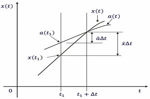
and
(5)
where and
are first-order derivatives of
and
, respectively.
shows the relationship of EquationEquation 12(12)
(12) in a Euclidean space
. The mean number
of upcrossing events can be represented by the shaded region. Since both
and
are stochastic processes, this shaded region is the probability content under the joint PDF
for
and
.
Figure 2. Integration limits in a plane.
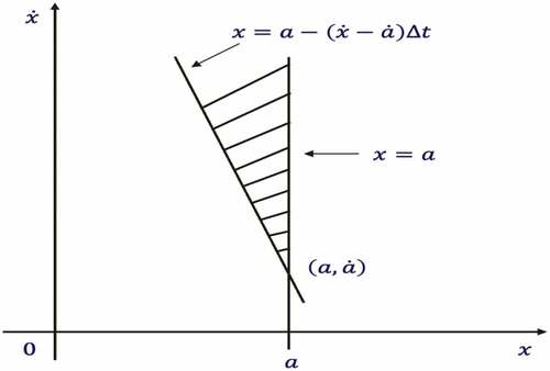
When , the shaded region becomes a narrow strip,
. The upcrossing rate
for
with a barrier
can be determined as follows
The above equation is the well-known Rice formula, which is an ensemble average upcrossing rate for all realizations of upcrossing a barrier level
at time
. However, deriving an analytical solution to
is difficult when
is not Gaussian or not completely continuous,
is nonlinear, and
is not convex polyhedral. Considerable efforts have been made to overcome these difficulties, centred at the transformation of general
to continuous Gaussian processes (Grigoriu, Citation1984; Winterstein, Citation1988) and the linearization of
(C. Q. Li, Citation1995). Besides, separation method (Rackwitz, Citation1984) is also used to separate the determination of
into those by continuous and discontinuous processes. Unions and intersections of component planar regions (Rackwitz, Citation1984) or spherical regions (Veneziano, Cornell, & Grigoriu, Citation1977) are used when the
is not convex polyhedral. However, since such modified
is often very conservative, it can result in an overestimated
.
2.3. PHI2+ method
Based on a two-component parallel system model, PHI2+ method determines as follows (Hagen & Tvedt, Citation1991)
Introducing a function and since
cannot satisfy the requirements
and
at the same time
,
. It follows that
can be re-written as follows
where . Since
is a two-component parallel system, it can be expressed as a bi-Gaussian cumulative function (Ditlevsen & Madsen, Citation1996).
can be derived as follows
where is the magnitude of a vector. For a stationary process,
and
, EquationEquation 12
(12)
(12) reduces to
.
It may be noted that, in PHI2+ method, a two-component parallel system is used to equate failure rate to upcrossing rate . Although failure rate can be equivalent to upcrossing rate within a small-time increment
, they are slightly different in concept. Because the upcrossing rate is driven by
as input whilst failure rate is governed by
as outputs (responses). Whilst the assumption of independent upcrossing events for
as input can be close to truth with not-too-narrow bandwidth and very high barrier level, the same assumption for failure events as response, e.g.,
, may need more qualification. Furthermore, whilst it might be accepted that inputs can be assumed, it is hardly acceptable for responses. PHI2+ method is accurate and efficient when
is a Gaussian process and
is linear. Otherwise, approximation is needed either in transformation of
to a standard Gaussian process or in determination of the reliability indexes for nonlinear
. Numerical tools seem to be inevitable and hence PHI2+ method is referred to as a hybrid method in this paper.
To improve the efficiency of PHI2+ method, moments-based transformation methods have been employed using the first few moments of . The contribution of introducing moments-based transformation methods in PHI2+ is to avoid finding the design points. Although the first few moments of
can be determined accurately for linear limit state functions, numerical methods, e.g., point estimate method, is often required for complicated
, which inevitably introduces approximation and simplification. Another issue of the moments-based transformation methods is the determination of inverse functions, for which Zhao and Lu (Citation2007) developed a simple explicit third-order polynomial function to avoid the nonlinear solution to polynomial coefficients.
Solutions for the analysis of time-dependent structural reliability are classified into 4 groups, i.e., analytical, hybrid, quasi and simulation solutions, which are analysed and discussed in the Sections 3-6. To have a clear understanding and easy reading, a simple summary of classification and methods for these solutions are shown in .
Table 1. A summary of classification and methods for time-dependent reliability.
. A summary of classification and methods for time-dependent reliability
3. Analytical solutions for time-dependent reliability
Existing analytical solutions to are mainly derived based on the Rice formula. For stationary Gaussian processes, analytical solutions to
are well-developed, e.g., Ditlevsen (Citation1983), Lindgren (Citation1980), Veneziano, Cornell, and Grigoriu (Citation1977), for various
or problems. Thus, only analytical solutions to
for nonstationary and/or non-Gaussian processes are of interest in the review.
3.1. Solutions for nonstationary processes
Practical observations show that the basic variables , e.g., applied loads and structural resistance, for structures are usually nonstationary processes, e.g., earthquakes, wind, ocean waves, material degradation, etc. (Papadimitriou, Citation1991). It is however difficult to derive an analytical solution to
for a nonstationary process due primarily to the correlation of
including autocorrelation, and correlation between
and its time derivative
. As a result, the analytical solutions to
for nonstationary processes are scarce.
C. Q. Li and Melchers (Citation1993) derived an analytical solution to for a nonstationary Gaussian vector process out of a convex polyhedral safe domain. This solution was developed based on the conditional probability of
, which effectively decorrelates
from
. Then the multi-dimensional integral of
reduces to one-dimensional one. For a linear
, Li and Melchers’ solution is a closed form, i.e., exact solution. For nonlinear ones, since the safe domain
needs to be linearized as convex polyhedrons, it is approximate, and its accuracy depends on how
is linearized. Moreover, since both the first and second order derivatives of multiple statistical parameters need to be determined, this solution is mathematically intensive.
To overcome the mathematical difficulties, Firouzi, Yang, and Li (Citation2018) derived a simpler and more efficient analytical solution to for a nonstationary Gaussian process out of a time-variant barrier. This solution improves the computational efficiency through making a reasonable approximation on the second order derivatives of Gaussian autocorrelation function and Sinus cardinal autocorrelation function (E. Vanmarcke, Citation2010), based on the L’Hopital’s rule (Zwillinger, Citation2018).
for a nonstationary Gaussian process is derived as follows (Firouzi, Yang, & Li, Citation2018)
where is the autocorrelation function of
,
is the second-order derivatives of
and
is the correlation length of
.
Firouzi, Yang, and Li (Citation2018)’s solution was applied to determine the probability of fracture failure of cast-iron pipes, in which the internal water pressure was simulated by a nonstationary Gaussian process. The results proved that this solution could transform a complex time-dependent reliability problem into a simple one with accuracy verified by MCS. In the examples demonstrated, the barrier level was a deterministic value, i.e., a constant fracture toughness value. However, for a random
, the local upcrossing rates which are conditional on the samples of
need to be first determined and then integrated over the whole random barrier to obtain the total upcrossing rate. For this purpose, other methods, e.g., asymptotic methods (Breitung, Citation1988; Rackwitz, Citation2001), need to be used.
3.2. Solutions for nonstationary and non-Gaussian processes
As it is known, both and structural responses or
are usually nonstationary and non-Gaussian processes. This further complicates the determination of
. Compared with nonstationary Gaussian processes, analytical solutions to
for nonstationary and non-Gaussian processes are extremely rare except a recent one by C. Q. Li, Firouzi, and Yang (Citation2016) even though it is for specific lognormal processes.
C. Q. Li, Firouzi, and Yang (Citation2016) derived a closed-form solution to for a scalar nonstationary lognormal process. In deriving the solution, the joint probability density function
between a stochastic process
and its derivative process
is separated, using conditional probability, as
. Based on the Rice formula,
for a scalar nonstationary lognormal process is derived as follows
The solution of C. Q. Li, Firouzi, and Yang (Citation2016) eliminated the negative values of Gaussian distribution, which was significant for the application of TdR methods in engineering practices involving many non-negative parameters. In the example demonstrated by C. Q. Li, Firouzi, and Yang (Citation2016), the derived solution was used for assessing the corrosion-induced cracking in concrete structures and the crack width was modelled as a nonstationary lognormal process. The cracking failure predicted by the derived solution was in good agreement with that of MCS and more accurate than that of safety index methods. Also, there is no assumption or manipulation of parameter values in calculating the upcrossing rate, which was practically important for this solution to be used in real structures. Besides, the influence of correlation coefficient functions of stochastic processes can be avoided due to the conditionality. However, this solution was only applicable for the problems with a deterministic barrier and single limit sate function. Also, since the stochastic process considered as was scalar, it was difficult for this solution to be extended for vector processes.
4. Hybrid solutions for time-dependent reliability
4.1. Parallel system model-based solution
PHI2+ method is developed based on a two-component parallel system model (Sudret, Citation2008). The derivation process of is analytical but determining the reliability index
, which is a key step, is numerical and hence it is referred to as a hybrid solution. The difficulty of determining
is to determine the design points, for which numerical methods are required for the repeatedly partial differentiations of
. This is computationally cumbersome and not easily applicable for engineering practice. Besides, the accuracy of this method depends on the linearity of
.
To simplify this, X. Y. Zhang, Lu, Wu, et al. (Citation2021) proposed a moment-based PHI2 method (referred as MPHI2) through using the first few moments of to calculate the required reliability indexes and hence
can be determined as follows
where and
are the reliability indexes at fixed points in time
and
respectively and
is the correlation coefficient between these two consecutive limit state functions.
To verify the MPHI2 method, a three-bay-six-story frame was used as an example and different methods, e.g., FORM-PHI2, SORM-PHI2, MCS and MPHI2 methods were used for comparison. In this example, the horizontal static loads were modelled as Gumbel processes. The results obtained from SORM-PHI2 and MPHI2 methods agreed well with the results of MCS. In comparison, the FORM-PHI2 method was less accurate. The MPHI2 method was superior to SORM-PHI2 method in the computational efficiency. It because that the time instant reliability indexes determined in MPHI2 method was separated from TdR cycle through using the statistical moments of a limit state function at successive time instants. However, for a nonstationary process, the statistical moments need to be estimated at different time points and the computational efficiency of MPHI2 method would be diminished. Furthermore, since MPHI2 method was developed based on the statistical moments, the accuracy of it strongly depends on the estimation of moments which was usually inaccurate when highly non-Gaussian processes are considered (Xu & Rahman, Citation2004).
As an improvement, Cai, Lu, Leng, et al. (Citation2021) proposed another hybrid solution based on PHI2+ method proposed by Sudret (Citation2008) and moment-based transformation method proposed by X. Y. Zhang, Lu, Wu, et al. (Citation2021). Cai, Lu, Leng, et al. (Citation2021)’s method was applied to investigate the reliability of a steel frame structure with horizontal and vertical loads modelled as a nonstationary Gamma and Lognormal process, respectively. The accuracy of this method was verified by MCS. In comparison with MCS, it was more computationally efficient. This method was also applied to assess the cracking failure of corroded-induced concrete structures, in which the crack width was modelled as a nonstationary Lognormal process. It was found that Cai, Lu, Leng, et al. (Citation2021)’s method was more applicable for the assessment of deteriorating structures over a long-time period. However, this method was not effective for problems with strong non-Gaussian processes and nonlinear limit state functions since it was difficult to obtain the higher-order moments and correlation functions for such limit state functions.
4.2. Moment-based transformation solution
Both PHI2+ and MPHI2 methods perform reasonably well in terms of accuracy and efficiency for Gaussian processes and linear . For non-Gaussian processes, various methods have been developed to transform them into Gaussian processes through distribution families or moment-based transformation methods. Although the distribution families, e.g., Burr system, John system, Pearson system and Lambda distribution (Grigoriu, Citation1982; Kleiber & Kotz, Citation2003; Ramberg & Schmeiser, Citation1974), can be used, the computation cost is too high. Thus, the moment-based transformation methods are often used.
For example, Winterstein (Citation1988) proposed what is now known as Winterstein’s polynomials method to transform a non-Gaussian process to an equivalent one based on the Hermite polynomials. This method can separately consider the softening processes (wider tails than Gaussian process, e.g., kurtosis ) and hardening processes (narrower tails than Gaussian process, e.g.,
). However, since the transformation process is non-monotonic for some combination of skewness and kurtosis, the Hermite coefficients for hardening processes cannot be given explicitly (Low, Citation2013). This limits the application of Winterstein ’s method, in particular, for a non-Gaussian process with hardening processes and strong non-Gaussianity.
To overcome this limitation, Zhao and Lu (Citation2007) proposed an explicit third-order polynomial transformation method, in which the polynomial coefficients are estimated based on the first four moments of stochastic processes. X. Y. Zhang, Zhao, and Lu (Citation2019) further developed a unified third order Hermite polynomial transformation method. Although these two methods are accurate for both hardening and softening processes, estimation of first four moments for complex limit state functions are difficult, if not impossible, and numerical tools are required.
4.3. Effect of bandwidth
It should be noted that EquationEquation 4(4)
(4) is accurate only when the individual upcrossing events are independent and only one upcrossing event occurs within an infinitesimal time increment. These require that the failure or crossing is a very rare event and the bandwidth of
is not-too-narrow (Naess, Citation1990). The issue of rare failure or crossing can be designed out and indeed the
of professionally designed structures is very small, e.g.,
. However, for a narrow-banded
, since the upcrossings from a threshold tend to occur in clumps, the assumption of an independent Poisson distribution for upcrossing events becomes not valid, which will cause underestimation of the upcrossing rate.
To overcome this limitation and reduce the errors caused by the narrow-banded , some correction methods have been developed for stationary Gaussian processes (E. H. Vanmarcke, Citation1975; Langley, Citation1988; Yi & Song, Citation2021) and non-Gaussian processes (He & Zhao, Citation2007; Naess, Citation1990; Zhao, Zhang, Lu, et al., Citation2019). For example, Naess (Citation1990) derived a simple and explicit closed-form expression to estimate the upcrossing rate and extreme value of a narrow-banded stationary non-Gaussian process. It employs the mean joint upcrossing rate to account for the effect of narrow bandwidth on the determination of upcrossing rates. However, since the different upcrossing events occurred in clumps are assumed to have a same dependence structure, this expression does not consider the effect of different types of dependence structure on the determination of upcrossing rates (Hu & Du, Citation2013). He and Zhao (Citation2007) proposed a moment-based correction method to consider the effect of narrow bandwidth on upcrossing rates through employing the concept of clump size (Langley, Citation1988). Even though this method can relax the assumption of independent Poisson distribution for the determination of upcrossing rates, it is not applicable for a non-Gaussian process with hardening processes because the Winterstein’s polynomials are used. To overcome this limitation, Zhao, Zhang, Lu, et al. (Citation2019) further proposed a fourth moment-based correction method, in which an explicit third-order polynomial transformation method was used. In comparison, Zhao, Zhang, Lu, et al. (Citation2019)’s method is more accurate for non-Gaussian processes with both hardening and softening processes. However, its accuracy decreases with the increase of dependence between the upcrossing events. Besides, it is difficult to estimate the high-order moments of limit state functions with highly non-Gaussian processes involved. Yi and Song (Citation2021) proposed a Poisson branching process (PBP) model to consider the statistical dependence between the crossing events occurred in the narrowband processes. It was proved that this PBP model-based formulation performs well on the stochastic processes with various shape of power spectral density and bandwidth parameters. Also, Yi and Song (Citation2021)’s formulation is effective for a wide range of threshold levels. However, its application is limited to the stationary Gaussian processes.
5. Quasi-solutions for time-dependent reliability
The extreme value-based methods can eliminate the time effect from the structural response or through replacing
with its extreme values. As a result, a time-dependent reliability problem is converted into a time-independent counterpart, which can be solved by, e.g., FORM/SORM. For this reason, extreme value-based methods are referred to as quasi time-dependent methods in this paper.
The key step of this method is to identify the extreme value of
over a given time period
(He, Citation2015). Then
can be defined as the probability when
is less than an acceptable limit (e.g., usually zero). With this method the random nature of
remains because the extreme value is a random variable. However, extreme values are mathematically intractable in most cases, especially for complex
. By employing a saddle point approximation technique, Hu and Du (Citation2013) developed a sampling method to estimate the cumulative distribution function (CDF) of extreme values of
(implicit with respect to time) with only one
. In their method,
is firstly discretised and then sample paths of
are obtained from the independent standard Gaussian variables generated by MCS. With the obtained extreme values from each sample path of
, the CDF of these extreme values can be determined by the saddle point approximation method.
Hu and Du (Citation2013) applied this sampling method to investigate the probability of failure of hydrokinetic turbine blades, in which the river flow velocity was modelled as a narrow-banded nonstationary Gaussian load process, i.e., a general stress variable. Compared with Rice formula-based methods, Hu and Du (Citation2013)’s method was more accurate since the assumption of independence upcrossing events was completely removed for narrow-banded stochastic processes. Also, it was more computational efficient because the number of evaluations of limit state functions was significantly reduced. However, the application of this method was limited to a limit-state function which was implicit with respect to time and contained only one nonstationary Gaussian process, e.g., either a general strength or a general stress variable.
To further improve the estimation efficiency of extreme value functions, Wang and Chen (Citation2017) developed a confidence-based adaptive extreme response surface (AERS) method. In this method, a spectral decomposition method is used to discretise by a set of independent standard Gaussian variables with deterministic orthogonal functions. Since
is expressed as a function of only random variables
and time
, a set of Gaussian processes are then constructed as the surrogate models to predict the instantaneous values of discretised
at all time-points. Besides, a confidence level is developed based on an adaptive sampling technique to identify critical time nodes for updating surrogate models.
Wang and Chen (Citation2017) also applied their developed method to predict the probability of failure of hydrokinetic turbine blades with the river flow velocity modelled as a narrow banded nonstationary Gaussian process. In comparison with the results obtained by PHI2+ method (Sudret, Citation2008) and MCS, this new developed method was more accurate. This was because that the dependence between the upcrossing events can be considered through tracking the evolution of stochastic processes by AERS approach. Also, it was more efficient than PHI2+ method since the adaptive sampling technique could identify the critical time nodes for reliability assessment. However, the application of this method was also limited to a nonstationary Gaussian process.
More recently, a more efficient time-variant extreme-value event evolution method (TEEM) was developed by Ping, Han, Jiang, et al. (Citation2019). In this method, an improved orthogonal series expansion method is used to simplify the representation of . Also, a series of extreme value events are obtained through discretising the time domain, which has a stable probability density function over time. As a result, the time history process of these obtained extreme value events can be simulated by a time-dependent polynomial chaos expansion method in terms of a function of standard Gaussian variables and time.
Ping, Han, Jiang, et al. (Citation2019) applied TEEM to evaluate the reliability of a printed circuit board module, whose service-life was mainly affected by the thermal deformation of chips. In their example, the thermal deformation of chips was modelled as a stationary Gaussian process. Compared with PHI2 method, TEEM was more accurate and computational efficient. However, TEEM is also only applicable for Gaussian processes. Clearly, future studies should consider more non-Gaussian processes.
6. SIMULATION SOLUTIONS for TIME-DEPENDENT RELIABILITY
In most cases, the probability of structural failure cannot be easily determined by methods reviewed in previous sections, mainly due to either complicated joint probability density functions of or complex
or both, not to mention the unavailability of either or both. In addition,
may involve multivariate variables with non-Gaussian distributions and the corresponding TdR problems can involve correlated stochastic processes. In these circumstances, MCS appears to be the only currently available method for accurately solving TdR problems which involve a wide range of
and complicated
.
However, the rationale of using MCS for determining greatly relies on whether the generated sample functions can be accurately represented, which may be either stationary or nonstationary, Gaussian or non-Gaussian, univariate or multivariate. There are many methods developed for simulating
, e.g., turning bands method (Der Kiureghian & Ke, Citation1988), optimal linear estimation method (C. C. Li & Der Kiureghian, Citation1993), orthogonal series expansion (OSE) method (J. Zhang & Ellingwood, Citation1994), expansion optimal linear estimation (EOLE) method (C. C. Li & Der Kiureghian, Citation1993), spectral representation method (SRM) (Shinozuka, Citation1971) and Karhunen-Loève (K-L) expansion-based method (Ghanem & Spanos, Citation2003; Kim & Shields, Citation2015; Zheng & Dai, Citation2017) etc. Among these methods, SRM and K-L are the most widely used methods due to their versatility and robustness, which will be specifically reviewed in the following sections together with EOLE and extended version of SRM for simulating correlated stochastic processes.
6.1. Expansion optimal linear estimation method
The expansion optimal linear estimation (EOLE) method was initially proposed by C. C. Li and Der Kiureghian (Citation1993) to solve problems with materials exhibiting random spatial variability and then used to simulate (D. Zhang, Han, Jiang, et al., Citation2017). EOLE method simulates a Gaussian process through solving the optimal linear estimation problem. To simulate a non-Gaussian process, the transformation procedures e.g., Grigoriu’s transformation (Grigoriu, Citation1984) and Nataf transformation (C. C. Li & Der Kiureghian, Citation1993) need to be used.
One advantage of EOLE method is that it can provide analytical expressions for the realization of . Another one is that the representation of
is optimal for Gaussian processes in the sense that it minimizes the errors in the variance at any given time point since Gaussian variables are used for a linear expression. Due to this reason, EOLE method is more efficient than some series expansion methods in the simulation of stationary Gaussian processes (D. Zhang, Han, Jiang, et al., Citation2017). Also, EOLE method is simple and readily implementable for problems in which failure events need to be defined over a spatial domain (Der Kiureghian & Zhang, Citation1999; Mirfendereski, Citation1995).
However, the accuracy of EOLE method depends on the type of autocorrelation functions. A finer discretization leads to an increase of correlation matrix size, which causes a high computation cost. Also, the stochastic process simulated by EOLE method underestimates the true variance of the target process since truncation often needs to be used. The numerical examples of Sudret and Der Kiureghian (Citation2000) show that the point-wise error of EOLE method for a given truncation number is generally larger than K-L expansion method. For these reasons, EOLE method is not widely used.
6.2. Spectral representation method
Spectral representation method (SRM) was firstly developed by Shinozuka (Citation1971) to simulate the problems with multidimensional, multivariate and nonstationary processes. The theoretical basis of SRM is the spectral representation theorem, by which can be decomposed into a series of sine or cosine random waveforms with random amplitudes. For a stationary Gaussian process, ergodic sample functions are generated, and the power spectra of them are identical to the corresponding prescribed power spectra. This is a major advantage of SRM as it is not necessary to reproduce the prescribed PSD information through a computationally expensive ensemble average.
Yamazaki and Shinozuka (Citation1988) advanced SRM and developed an iterative procedure to simulate a non-Gaussian stochastic process as shown in . This simulation procedure assumes an initial power spectral density (PSD) function of a Gaussian process and generates its corresponding sample function. Then transform the simulated Gaussian process into a non-Gaussian process based on Grigoriu’s theory (Grigoriu, Citation1995). This method uses an iterative procedure to update initially assumed PSD until it converges to the target PSD. And the updated PSDs are used for generate sample functions of the target non-Gaussian process.
Figure 3. Flow chart of simulation procedure of a non-Gaussian process by SRM and its application in TdR problems (modified from Yamazaki & Shinozuka, Citation1988).
This method shows high accuracy in terms of matching the marginal PDF of the generated non-Gaussian sample functions into the target marginal PDF for slightly skewed stochastic processes. However, since the Gaussianity of the underlying Gaussian process changes during the iteration process, it will cause the marginal PSD of the target non-Gaussian process does not match well when simulating non-Gaussian stochastic processes with highly skewed PDFs. To deal with this issue, Deodatis and Micaletti (Citation2001) modified the iteration procedure through determining the empirical (non-Gaussian) marginal PDF of the underlying stochastic process at each iteration step. This ensures that every generated sample function has the exact prescribed non-Gaussian marginal PDFs for each iteration. It was found that this method can accurately simulate non-Gaussian stochastic processes that are highly skewed.
In comparison, the spectral representation-based methods for simulating nonstationary and non-Gaussian stochastic processes are rare. It is because that it is difficult to determine a unique evolutionary spectrum (ES) for a stochastic process with known nonstationary autocorrelation functions. Shields and Deodatis (Citation2013) developed an approximate method to estimate the ES of a nonstationary Gaussian and/or non-Gaussian process. This method is found accurate in simulating most of nonstationary and non-Gaussian processes. However, its accuracy decreases as the degrees of non-stationarity and non-Gaussianity simultaneously increase. Also, it requires additional approximations in the estimation of ES, and a unique ES still cannot be determined. More recently, Benowitz, Shields, and Deodatis (Citation2015) studied the uniqueness of ES in simulating nonstationary and non-Gaussian processes. It is found that although a unique ES exists under certain conditions, an extremely high computation cost is required. This implies that simulation of nonstationary and non-Gaussian processes is still very difficult by the use of SRM.
6.3. Karhunen-Loève expansion method
Karhunen-Loève (K-L) expansion method is a bi-orthogonal stochastic process expansion, which provides a unified framework to simulate both the stationary and nonstationary stochastic processes (Ghanem & Spanos, Citation2003; Zheng & Dai, Citation2017). The main advantage of the K – L expansion method in simulating nonstationary Gaussian processes is that little additional effort is required because correlation functions do not need to be stationary. Phoon, Huang, and Quek (Citation2002, Citation2005) extended the K-L expansion method to simulate non-Gaussian processes based on an iterative mapping scheme. In this method, a specified marginal PDF that deviates significantly from the Gaussian process can be handled efficiently and the algorithm is found more robust (i.e., easier to converge) than the iterative scheme of Yamazaki and Shinozuka (Citation1988).
Kim and Shields (Citation2015) further proposed a K-L-based iterative translation approximation method to estimate the underlying Gaussian autocorrelation functions based on a nonstationary translation process theory. The main advantage of this method is that the iteration is directly performed on a nonstationary autocorrelation function. This avoids estimating the ES from nonstationary autocorrelation functions and alleviates the associated approximations as observed in the simulation of nonstationary and non-Gaussian processes by use of SRM (seen in Shields & Deodatis, Citation2013). Other advantages of Kim and Shields (Citation2015)’s method include that the underlying Gaussian ES can satisfy the compatibility conditions imposed by translation process theory and the computed non-Gaussian ES is very close to the target non-Gaussian one. However, this improvement in accuracy incurs high computational cost because autocorrelation functions are involved in the iteration process.
Recently, Dai, Zheng, and Ma (Citation2019) proposed a new method for simulating nonstationary and non-Gaussian processes based on both K-L expansion method and polynomial chaos expansion (PCE) method. The main procedure of this method is to represent the target stochastic process in the K-L series form first, and the random coefficients in the K-L series are subsequently decomposed using one-dimensional PCE method. The main advantage of this method is that the correlation function of the resulting stochastic process automatically matches the target one by virtue of the orthogonal property of Hermite polynomials, and one only needs to iterate the marginal PDF to match the target one. This, thus, provides an explicit and unified framework for simulating non-Gaussian processes with arbitrary correlation functions.
6.4. Simulation of correlated stochastic processes
The methods reviewed above focus on simulating a single (scalar) process and generalization to correlated (vector) processes is not straightforward (Cho, Venturi, & Karniadakis, Citation2013). Over the years, various methods have been developed for this purpose as extended versions of the original SRM and K-L expansion method. Taking SRM as an example, suppose a multivariate/correlated stationary process having mean value equal to zero with the cross-correlation matrix and cross-spectral density matrix given by
and
, respectively. The key step for simulating a correlated
is to decompose
and once
is decomposed, the ith process
can be simulated by SRM. However, high computer memories are required to simulate correlated processes by these methods.
To improve computational efficiency in both time and memory consumption, Chen and Letchford (Citation2005) proposed a hybrid approach that incorporates the proper orthogonal decomposition approach into SRM. The advantage of this method is that the number of variables of target correlated processes can be reduced through finding an optimal basis in the integrated cross power spectral density matrices. Vořechovský (Citation2008) further proposed a K-L expansion-based numerical method to generate correlated stochastic processes by use of a specified marginal distribution function, autocorrelation and cross-correlation structures. The main advantage of this method is that all correlated processes are expanded using the same spectrum of eigenfunctions or vectors, and computational effort can be significantly reduced since the decomposition of autocorrelation structure is performed only once. Also, Cho, Venturi, and Karniadakis (Citation2013) extended the application range of Vořechovský (Citation2008)’s method from correlated processes of same type to that of different types.
Furthermore, many other researchers, e.g., Lu et al. (Citation2020), Yang and Gurley (Citation2015) and Bocchini and Deodatis (Citation2008), simulated the correlated stationary non-Gaussian processes by transformation methods, which either utilise marginal probability density functions and the correlation function matrix (CFM) or the first four moments and CFM of the target non-Gaussian process. For example, the transformation method used by Lu et al. (Citation2020) is a unified Hermite polynomial model. The advantage of Lu et al. (Citation2020)’s method is that a wide range of stationary non-Gaussian processes can be simulated. However, this method is not straightforward when the translated Gaussian CFM becomes nonpositive definite during simulation because the power spectral density matrix of the underlying Gaussian needs to be modified. This not only involves some simulation errors but also increases the computational cost drastically. Also, this method together with others (e.g., Bocchini & Deodatis, Citation2008; Yang & Gurley, Citation2015) are only applicable for stationary processes. Simulating correlated nonstationary and non-Gaussian process is still a challenging at the present.
7. Challenges and future outlook
shows solutions revised in the paper for various methods which is followed to further explore the future challenges and directions in TdR methods. For consistency, since all the existing analytical solutions for TdR analysis are based on Rice-formula, the challenges and future directions are presented collectively whilst other three solutions, i.e., hybrid, quasi and simulation, are presented individually.
7.1. Analytical solutions
Analytical solutions have the advantage of facilitating wider applications of TdR methods and hence are of special interest to both academics and practitioners. Deriving a more accurate and robust analytical solution for general stochastic processes, neither stationary nor Gaussian, is a future direction for TdR theory. This would certainly increase or promote the application of TdR methods in engineering practice. However, there are mainly three kinds of challenges in deriving analytical solutions, which are discussed below.
Firstly, the Rice formula-based analytical solutions are by and large applicable for Gaussian processes since the joint multi-dimensional probability density functions (PDFs) for non-Gaussian processes are very difficult to be obtained. Even though several approximation methods, such as Lind and Hong (Citation1991), Huang and Long (Citation1980), have been developed. These methods are not effective for strongly non-Gaussian processes. Therefore, in the future studies, it is necessary to derive analytical solutions for non-Gaussian processes. For example, some processes, such as Gamma and extreme value processes, are neither stationary nor Gaussian but with known PDFs. The analytical solutions for these processes still have not been developed. Deriving analytical solutions for these processes can be one of future directions.
Secondly, due to the Poisson assumption made in its derivation, Rice formula-based analytical solutions are approximate but conservative. Experience and observation in applying these solutions indicate that they are sufficiently accurate for reliability assessment of professionally designed structures. It is therefore not a necessity nor inevitability to further develop Rice formula-based analytical solutions without any assumption. For academic endeavour, however, attempts have been made to derive analytical solutions without the Poisson assumption, such as Zhao, Zhang, Lu, et al. (Citation2019), He and Zhao (Citation2007), Naess (Citation1990), but inevitably other kinds of assumptions or approximations are induced, such as independence structures. As a future direction for research, the Poisson assumption can be eliminated by considering the dependence between outcrossing events. For example, the effects of narrow-banded stochastic processes and lower barrier levels on the calculation of outcrossing rate can be considered.
Finally, the barrier level used in deriving Rice formula-based analytical methods and their various versions, is deterministic. When the barrier is a stochastic process, the Rice formula needs to be modified as attempted by C. Q. Li and Melchers (Citation1993) but its complication is obvious. In this case, asymptotic methods need to be employed. Therefore, in the future study, the stochastic nature of the barrier level can be considered in deriving analytical solutions.
7.2. Hybrid solutions
PHI2+ method is a considerable improvement for obtaining upcrossing rate but its accuracy is affected by the nonlinearity of due to approximation methods, such as FORM/SORM, employed for determining the instantaneous reliability indexes at each design point. Numerical methods, such as Hasofer-Lind-Rackwitz-Fiessler algorithm and sequential quadratic programming, are required to determine the design points if
is highly nonlinear. This will decrease the efficiency of PHI2+ method due to repeated partial differentiation of
. Also, the non-Gaussianity of
can affect the accuracy of PHI2+ method. This situation can be worse if
contains dependent variables. Moreover, with the employment of a two-component parallel system model in PHI2+ method, the trajectory of
is not considered, in particular, its correlation. In the future studies, it would be desirable that an efficient method can be developed for the determination of reliability indexes of highly nonlinear
involving correlated stochastic processes. For example, an efficient transformation model can be combined with PHI2+ method, in which a non-Gaussian process can be transformed into a standard one with high accuracy, especially for strongly non-Gaussian processes.
The moment-based transformation methods work with PHI2 method to simplify the determination of reliability indexes. However, the accuracy and efficiency of moment-based transformation methods rely on the estimation of first few moments and correlation functions of , which is difficult for a highly nonlinear
, especially with non-Gaussian processes. In addition, numerical methods, e.g., point estimate method, can increase the computational cost and hence reduces the otherwise advantageous computational efficiency. More research is needed for the accurate estimation of higher-order moments and correlation functions of highly nonlinear
with strongly nonstationary and/or non-Gaussian processes. It is expected that the moment-based transformation methods can be coupled with PHI2+ method better than with PHI2 method. As such this can be a good future direction with perhaps more improvements of both moment-based transformation methods and PHI2+ method. Furthermore, the reliability indexes required for PHI2+ method should be directly determined from the moment-based transformation methods, which can improve the computation efficiency of PHI2+ method.
7.3. Quasi-solutions
Since the extreme value-based methods can convert TdR problems into a time-independent counterpart, TdR problems can be solved by time-independent reliability methods, e.g., FORM and SORM. Compared with upcrossing rate-based methods (including the analytical solutions and hybrid solutions), the extreme value-based methods are more accurate for narrow-banded stochastic processes. It because that the Poisson distribution assumption made in upcrossing rate-based methods can be removed. However, constructing an effective model to accurately estimate the extreme value distributions of stochastic processes is still a challenge. Besides, even though the efficiency and accuracy of extreme value-based methods can be improved by optimizing the models used for identifying extreme value distributions, their application are only available for a nonstationary Gaussian process. Extending the application of extreme value-based methods from stationary or nonstationary Gaussian processes to nonstationary and non-Gaussian processes can be a future direction. There are various developed moment-based transformation methods (Zhao & Lu, Citation2021) that can be combined with the extreme value-based methods. If the first few moments are determined to represent the probabilistic distributions of nonstationary and non-Gaussian processes, it is possible to simplify the identification procedure of extreme value distributions of these stochastic processes. Besides, it would be good to see that the limit state function can contain multiple stochastic processes.
7.4. Simulation solutions
Compared with analytical solutions, MCS-based methods for time-dependent reliability have developed more rapidly, attributing to the development of computing techniques. The accuracy of simulated stochastic processes is the pivot to these methods.
The generalised form of spectral representation-based method for simulating correlated processes often require high computer memories and the simulation process is often very slow, which are caused by the estimation of unique evolutionary spectrum. Although recent developed methods can be used to simulate correlated stationary non-Gaussian processes (Lu et al. Citation2020), their practicality may still be limited since intensive computational effort is required. Also, simulating correlated nonstationary and non-Gaussian process is still a challenge at present. Therefore, as a future direction, an efficient and robust numerical program can be developed to accurately simulate multivariate and correlated nonstationary and non-Gaussian processes widely involved in time-dependent reliability problems.
The main advantage of the K – L expansion-based methods is that it can be easily generalised to simulate nonstationary processes with little additional effort since the covariance functions do not need to be stationary. This method also has an advantage over the spectral representation-based methods for strongly correlated processes. The K-L-based iterative translation approximation method (Kim & Shields, Citation2015) can avoid estimating the evolutionary spectrum from the nonstationary autocorrelations and the associated approximations, which is recognised as one of few most accurate methods although not the most efficient one. However, main factors influencing the efficiency of K-L expansion-based method are the necessity of numerically solving the Fredholm integral equation. It is proposed that an analytical pre-processing step of the eigen-solution can be used to reduce the computational cost while ensuring its accuracy.
In summary, although the EOLE-based methods, spectral representation-based methods and K-L expansion-based methods can be used for the simulation of stationary and nonstationary Gaussian processes with high accuracy, they are not accurate enough for simulating nonstationary and non-Gaussian processes, especially with increasing non-stationarity and non-Gaussianity. It would be desirable that an effective simulation method can be developed for the simulation of highly nonstationary and non-Gaussian processes with a low computation cost.
8. Conclusions
This paper has critically reviewed the methods for time-dependent reliability (TdR) with a focus on analytical, Hybrid and simulation solutions. It is found in the review that: 1) Analytical (Rice formula-based) solutions are analytically derived and provide accurate solutions to upcrossing rates, but the solutions are limited to nonstationary Gaussian and lognormal processes. Further research can focus on solutions for more general nonstationary and non-Gaussian processes and their effective application for practitioners; 2) Hybrid (parallel system model-based) solutions are derived with a combined analytical and numerical techniques which provide effective solutions to upcrossing rates, but the solutions are affected by non-Gaussianity and nonlinearity of limit state functions. Further research can focus on the accuracy and efficiency for highly non-Gaussian process and nonlinear limit state functions; 3) Simulation (MCS-based) solutions provide robust solutions to upcrossing rates, but the accuracy and efficiency of these methods rely on the simulation of stochastic processes. Further research can focus on the accurate description of correlation for nonstationary and non-Gaussian processes and the efficiency of their simulations. It is also found that the effectiveness of all commonly used TdR methods, as reviewed in the paper, depends highly on the complexity of limit state functions and types of stochastic processes involved, in particular, the stationarity, Gaussianity and correlation. It can be concluded that, whilst significant progress has been achieved in the field of reliability theories and methods, there is still space to advance this knowledge and TdR has shown the potential to lead this advancement.
Acknowledgments
Financial support from the Australian Research Council under DP230100983 and DP170102211 is gratefully acknowledged.
Disclosure statement
No potential conflict of interest was reported by the author(s).
Additional information
Funding
Notes on contributors
Bohua Zhang
Bohua Zhang, PhD Candidate, School of Engineering, RMIT University, Melbourne, Australia
Weigang Wang
Weigang Wang, Research fellow, School of Engineering, RMIT University, Melbourne, Australia
Yanlin Wang
Yanlin Wang, Research Assistant, School of Engineering, RMIT University, Melbourne, Australia
Yueru Li
Yueru Li, PhD Candidate, School of Engineering, RMIT University, Melbourne, Australia
Chun-Qing Li
Chun-Qing Li, Professor, School of Engineering, RMIT University, Melbourne, Australia
References
- Andrieu-Renaud, C., Sudret, B., & Lemaire, M. (2004). The PHI2 method: A way to compute time-variant reliability. Reliability Engineering & System Safety, 84(1), 75–86. https://doi.org/10.1016/j.ress.2003.10.005
- Benowitz, B. A., Shields, M. D., & Deodatis, G. (2015). Determining evolutionary spectra from non-stationary autocorrelation functions. Probabilistic Engineering Mechanics, 41, 73–88. https://doi.org/10.1016/j.probengmech.2015.06.004
- Bocchini, P., & Deodatis, G. (2008). Critical review and latest developments of a class of simulation algorithms for strongly non-Gaussian random fields. Probabilistic Engineering Mechanics, 23(4), 393–407. https://doi.org/10.1016/j.probengmech.2007.09.001
- Breitung, K. (1988). Asymptotic crossing rates for stationary Gaussian vector processes. Stochastic Processes and Their Applications, 29(2), 195–207. https://doi.org/10.1016/0304-4149(88)90037-3
- Cai, C. H., Lu, Z. H., Leng, Y., Zhao, Y. G., & Li, C. Q. (2021). Time-dependent structural reliability assessment for nonstationary non-Gaussian performance functions. Journal of Engineering Mechanics, 147(2), 04020145. https://doi.org/10.1061/(ASCE)EM.1943-7889.0001883
- Chen, L., & Letchford, C. W. (2005). Simulation of multivariate stationary Gaussian stochastic processes: Hybrid spectral representation and proper orthogonal decomposition approach. Journal of Engineering Mechanics, 131(8), 801–808. https://doi.org/10.1061/(ASCE)0733-9399(2005)131:8(801)
- Cho, H., Venturi, D., & Karniadakis, G. E. (2013). Karhunen–loève expansion for multi-correlated stochastic processes. Probabilistic Engineering Mechanics, 34, 157–167. https://doi.org/10.1016/j.probengmech.2013.09.004
- Cramer, H., & Leadbetter, M. R., 1967. Frequency detection and related topics: Stationary and related stochastic processes, Ch. 14.
- Dai, H., Zheng, Z., & Ma, H. (2019). An explicit method for simulating non-Gaussian and non-stationary stochastic processes by Karhunen-Loève and polynomial chaos expansion. Mechanical Systems and Signal Processing, 115, 1–13. https://doi.org/10.1016/j.ymssp.2018.05.026
- Deodatis, G., & Micaletti, R. C. (2001). Simulation of highly skewed non-Gaussian stochastic processes. Journal of Engineering Mechanics, 127(12), 1284–1295. https://doi.org/10.1061/(ASCE)0733-9399(2001)127:12(1284)
- Der Kiureghian, A., & Ke, J. B. (1988). The stochastic finite element method in structural reliability. Probabilistic Engineering Mechanics, 3(2), 83–91. https://doi.org/10.1016/0266-8920(88)90019-7
- Der Kiureghian, A., & Zhang, Y. (1999). Space-variant finite element reliability analysis. Computer Methods in Applied Mechanics and Engineering, 168(1–4), 173–183. https://doi.org/10.1016/S0045-7825(98)00139-X
- Ditlevsen, O. (1983). Gaussian upcrossings from safe convex polyhedrons. Journal of Engineering Mechanics, 109(1), 127–148. https://doi.org/10.1061/(ASCE)0733-9399(1983)109:1(127)
- Ditlevsen, O., & Madsen, H. O. (1996). Structural reliability methods (Vol. 178). Wiley.
- Firouzi, A., Yang, W., & Li, C. Q. (2018). Efficient solution for calculation of upcrossing rate of nonstationary Gaussian process. Journal of Engineering Mechanics, 144(4), 04018015. https://doi.org/10.1061/(ASCE)EM.1943-7889.0001420
- Ghanem, R. G., & Spanos, P. D. (2003). Stochastic finite elements: A spectral approach. Courier Corporation.
- Grigoriu, M. (1982). Approximate analysis of complex reliability problems. Structural Safety, 1(4), 277–288. https://doi.org/10.1016/0167-4730(82)90004-2
- Grigoriu, M. (1984). Crossings of non-Gaussian translation processes. Journal of Engineering Mechanics, 110(4), 610–620. https://doi.org/10.1061/(ASCE)0733-9399(1984)110:4(610)
- Grigoriu, M. (1995). Applied non-gaussian processes: Examples, theory, simulation, linear random vibration, and MATLAB solutions(Book). Prentice Hall, Inc.
- Hagen, Ø., & Tvedt, L. (1991). Vector process out-crossing as parallel system sensitivity measure. Journal of Engineering Mechanics, 117(10), 2201–2220. https://doi.org/10.1061/(ASCE)0733-9399(1991)117:10(2201)
- He, J. (2015). Approximate method for estimating extreme value responses of nonlinear stochastic dynamic systems. Journal of Engineering Mechanics, 141(7), 04015009. https://doi.org/10.1061/(ASCE)EM.1943-7889.0000901
- He, J., & Zhao, Y. G. (2007). First passage times of stationary non-Gaussian structural responses. Computers & Structures, 85(7–8), 431–436. https://doi.org/10.1016/j.compstruc.2006.09.009
- Huang, N. E., & Long, S. R. (1980). An experimental study of the surface elevation probability distribution and statistics of wind-generated waves. Journal of Fluid Mechanics, 101(1), 179–200.
- Hu, Z., & Du, X. (2013). A sampling approach to extreme value distribution for time-dependent reliability analysis. Journal of Mechanical Design, 135(7), 071003. https://doi.org/10.1115/1.4023925
- Kim, H., & Shields, M. D. (2015). Modeling strongly non-Gaussian non-stationary stochastic processes using the iterative translation approximation method and Karhunen–Loève expansion. Computers & Structures, 161, 31–42. https://doi.org/10.1016/j.compstruc.2015.08.010
- Kleiber, C., & Kotz, S. (2003). Statistical size distributions in economics and actuarial sciences (Vol. 470). John Wiley & Sons.
- Langley, R. S. (1988). A first passage approximation for normal stationary random processes. Journal of Sound and Vibration, 122(2), 261–275. https://doi.org/10.1016/S0022-460X(88)80353-5
- Li, C. Q. (1995). Computation of the failure probability of deteriorating structural systems. Computers & Structures, 56(6), 1073–1079. https://doi.org/10.1016/0045-7949(94)00947-2
- Li, C. C., & Der Kiureghian, A. (1993). Optimal discretization of random fields. Journal of Engineering Mechanics, 119(6), 1136–1154. https://doi.org/10.1061/(ASCE)0733-9399(1993)119:6(1136)
- Li, C. Q., Firouzi, A., & Yang, W. (2016). Closed-form solution to first passage probability for nonstationary lognormal processes. Journal of Engineering Mechanics, 142(12), 04016103. https://doi.org/10.1061/(ASCE)EM.1943-7889.0001160
- Li, C. Q., & Melchers, R. E. (1993). Upcrossings from convex polyhedrons for nonstationary Gaussian processes. Journal of Engineering Mechanics, 119(11), 2354–2361. https://doi.org/10.1061/(ASCE)0733-9399(1993)119:11(2354)
- Lindgren, G. (1980). Extreme values and crossings for the x 2-process and other functions of multidimensional gaussian processes, by reliability applications. Advances in Applied Probability, 12(3), 746–774. https://doi.org/10.2307/1426430
- Lind, N. C., & Hong, H. P. (1991). Tail entropy approximations. Structural Safety, 10(4), 297–306. https://doi.org/10.1016/0167-4730(91)90036-9
- Li, C. Q., & Yang, W. (2022). Time-dependent reliability theory and its applications. Elsevier.
- Low, Y. M. (2013). A new distribution for fitting four moments and its applications to reliability analysis. Structural Safety, 42, 12–25. https://doi.org/10.1016/j.strusafe.2013.01.007
- Lu, Z. H., Zhao, Z., Zhang, X. Y., Li, C. Q., Ji, X. W., & Zhao, Y. G. (2020). Simulating stationary non-Gaussian processes based on unified Hermite polynomial model. Journal of Engineering Mechanics, 146(7), 04020067. https://doi.org/10.1061/(ASCE)EM.1943-7889.0001806
- Melchers, R. E., & Beck, A. T. (2018). Structural reliability analysis and prediction. John wiley & sons.
- Mirfendereski, D., 1995. Stochastic modeling and response prediction of MEMS (Doctoral dissertation, University of California.
- Naess, A. (1990). Approximate first-passage and extremes of narrow-band Gaussian and non-Gaussian random vibrations. Journal of Sound and Vibration, 138(3), 365–380. https://doi.org/10.1016/0022-460X(90)90592-N
- Papadimitriou, K. M. (1991). Stochastic characterization of strong ground motion and applications to structural response. California Institute of Technology.
- Phoon, K. K., Huang, H. W., & Quek, S. T. (2005). Simulation of strongly non-Gaussian processes using Karhunen–Loeve expansion. Probabilistic Engineering Mechanics, 20(2), 188–198. https://doi.org/10.1016/j.probengmech.2005.05.007
- Phoon, K. K., Huang, S. P., & Quek, S. T. (2002). Simulation of second-order processes using Karhunen–Loeve expansion. Computers & Structures, 80(12), 1049–1060. https://doi.org/10.1016/S0045-7949(02)00064-0
- Ping, M. H., Han, X., Jiang, C., & Xiao, X. Y. (2019). A time-variant extreme-value event evolution method for time-variant reliability analysis. Mechanical Systems and Signal Processing, 130, 333–348. https://doi.org/10.1016/j.ymssp.2019.05.009
- Rackwitz, R. (1984). Failure rates for general systems including structural components. Reliability Engineering, 9(4), 229–242. https://doi.org/10.1016/0143-8174(84)90052-0
- Rackwitz, R. (2001). Reliability analysis—a review and some perspectives. Structural Safety, 23(4), 365–395. https://doi.org/10.1016/S0167-4730(02)00009-7
- Ramberg, J. S., & Schmeiser, B. W. (1974). An approximate method for generating asymmetric random variables. Communications of the ACM, 17(2), 78–82. https://doi.org/10.1145/360827.360840
- Rice, S. O. (1945). Mathematical analysis of random noise. Bell System Technical Journal, 24(1), 46–156. https://doi.org/10.1002/j.1538-7305.1945.tb00453.x
- Shields, M. D., & Deodatis, G. (2013). Estimation of evolutionary spectra for simulation of non-stationary and non-Gaussian stochastic processes. Computers & Structures, 126, 149–163. https://doi.org/10.1016/j.compstruc.2013.02.007
- Shinozuka, M. (1971). Simulation of multivariate and multidimensional random processes. The Journal of the Acoustical Society of America, 49(1B), 357–368. https://doi.org/10.1121/1.1912338
- Sudret, B. (2008). Analytical derivation of the upcrossing rate in time-variant reliability problems. Structure and Infrastructure Engineering, 4(5), 353–362. https://doi.org/10.1080/15732470701270058
- Sudret, B., & Der Kiureghian, A., 2000. Stochastic finite element methods and reliability: A state-of-the-artreport (pp. 18–34). Department of Civil and Environmental Engineering, University of California.
- Vanmarcke, E. (2010). Random fields: Analysis and synthesis. World scientific.
- Vanmarcke, E. H. (1975). On the distribution of the first-passage time for normal stationary random processes. Journal of Applied Mechanics, 42(1), 215–220. https://doi.org/10.1115/1.3423521
- Veneziano, D., Cornell, C. A., & Grigoriu, M. (1977). Vector-process models for system reliability. Journal of the Engineering Mechanics Division, 103(3), 441–460. https://doi.org/10.1061/JMCEA3.0002239
- Vořechovský, M. (2008). Simulation of simply cross correlated random fields by series expansion methods. Structural Safety, 30(4), 337–363. https://doi.org/10.1016/j.strusafe.2007.05.002
- Wang, Z., & Chen, W. (2017). Confidence-based adaptive extreme response surface for time-variant reliability analysis under random excitation. Structural Safety, 64, 76–86. https://doi.org/10.1016/j.strusafe.2016.10.001
- Winterstein, S. R. (1988). Nonlinear vibration models for extremes and fatigue. Journal of Engineering Mechanics, 114(10), 1772–1790. https://doi.org/10.1061/(ASCE)0733-9399(1988)114:10(1772)
- Xu, H., & Rahman, S. (2004). A generalized dimension‐reduction method for multidimensional integration in stochastic mechanics. International Journal for Numerical Methods in Engineering, 61(12), 1992–2019. https://doi.org/10.1002/nme.1135
- Yamazaki, F., & Shinozuka, M. (1988). Digital generation of non-Gaussian stochastic fields. Journal of Engineering Mechanics, 114(7), 1183–1197. https://doi.org/10.1061/(ASCE)0733-9399(1988)114:7(1183)
- Yang, L., & Gurley, K. R. (2015). Efficient stationary multivariate non-Gaussian simulation based on a Hermite PDF model. Probabilistic Engineering Mechanics, 42, 31–41. https://doi.org/10.1016/j.probengmech.2015.09.006
- Yi, S. R., & Song, J. (2021). First-passage probability estimation by Poisson branching process model. Structural Safety, 90, 102027. https://doi.org/10.1016/j.strusafe.2020.102027
- Zhang, J., & Ellingwood, B. (1994). Orthogonal series expansions of random fields in reliability analysis. Journal of Engineering Mechanics, 120(12), 2660–2677. https://doi.org/10.1061/(ASCE)0733-9399(1994)120:12(2660)
- Zhang, D., Han, X., Jiang, C., Liu, J., & Li, Q. (2017). Time-dependent reliability analysis through response surface method. Journal of Mechanical Design, 139(4), 041404. https://doi.org/10.1115/1.4035860
- Zhang, X. Y., Lu, Z. H., Wu, S. Y., & Zhao, Y. G. (2021). An efficient method for time-variant reliability including finite element analysis. Reliability Engineering & System Safety, 210, 107534. https://doi.org/10.1016/j.ress.2021.107534
- Zhang, X. Y., Zhao, Y. G., & Lu, Z. H. (2019). Unified Hermite polynomial model and its application in estimating non-Gaussian processes. Journal of Engineering Mechanics, 145(3), 04019001. https://doi.org/10.1061/(ASCE)EM.1943-7889.0001577
- Zhao, Y. G., & Lu, Z. H. (2007). Fourth-moment standardization for structural reliability assessment. Journal of Structural Engineering, 133(7), 916–924. https://doi.org/10.1061/(ASCE)0733-9445(2007)133:7(916)
- Zhao, Y. G., & Lu, Z. H. (2021). Structural reliability: Approaches from perspectives of statistical moments. John Wiley & Sons.
- Zhao, Y. G., Zhang, L. W., Lu, Z. H., & He, J. (2019). First passage probability assessment of stationary non-Gaussian process using the third-order polynomial transformation. Advances in Structural Engineering, 22(1), 187–201. https://doi.org/10.1177/1369433218782873
- Zheng, Z., & Dai, H. (2017). Simulation of multi-dimensional random fields by Karhunen–Loève expansion. Computer Methods in Applied Mechanics and Engineering, 324, 221–247. https://doi.org/10.1016/j.cma.2017.05.022
- Zwillinger, D. (2018). CRC standard mathematical tables and formulas. Chapman and hall/CRC.