Closed-form solutions of dynamic vibration equations of seismically excited structures

Abstract

Novel closed-form solutions of the dynamic vibration equations of seismically excited structures are derived by using the Laplace transform. Structures with single-degree-of-freedom (SDOF) and multi-degree-of-freedom (MDOF) are considered and modelled as lumped mass systems. Several earthquake records with different peak ground accelerations (PGAs) are used to excite such systems. To be compared, time-history responses are obtained numerically by using Newmark’s step-by-step iteration method and analytically by the proposed approach. After conducting such comparisons, the proposed approach successfully computes the exact responses of seismically excited structures.

Keywords:

• Closed-form solutions
• earthquake motion
• Laplace transform
• seismically excited structures
• seismic response

1. Introduction

An earthquake is one of the most severe and unexpected threats to a building structure. Thus, it is a substantial issue in the practical field and the research sector. Examples of significant earthquakes are L'Aquila (Italy 2009), Port-au-Prince (Haiti 2010), Lamjung (Nepal 2015), and Amatrice (Italy 2016). The structural seismic responses induced by such significant earthquakes may result in serious casualties or economic loss to human society. Many researchers made great efforts to enhance structural seismic responses and the influence of excitation parameters on such responses (Castaldo & Tubaldi, 2018; Hareen & Mohan, 2021; Hussain & Dutta, 2020).

Control systems that reduce the seismic response of towers, bridges, and buildings have drawn a lot of interest during the past twenty years. Control systems may be split into four groups: active, semi-active, hybrid, and passive systems. Although active and semi-active systems are implemented completely in several structures, their cost-effectiveness and reliability are limited in their acceptance. Conversely, hybrid and passive systems are accepted due to their low-power requirements and mechanical simplicity.

To dissipate seismic energy, passive devices such as tuned mass damper (TMD), base isolation, tuned liquid damper (TLD), and pendulum tuned mass damper (PTMD) are typically utilized and used in new constructions (Abd-Elhamed & Mahmoud, 2019a; Abd-Elhamed & Tolan, 2022). Rarely, they are used to protect pre-existed structures since they often need substantial changes to the original design. A tuned mass damper is a mechanical device whose mass is fastened to the building’s peak. Linear stiffeners or hangers in PTMD regulate the oscillating motion of the mass damper as well as linear energy dissipation devices. The stiffness and damping properties of TMD must be tuned to dissipate enough kinetic energy transmitted from a dynamically stimulated structure to the damper.

To safeguard structures from earthquake-related disasters, an analysis of their dynamical behaviour is necessary (Jia, Song, Xu, He, & Bai, 2015). Thus, a second-order ordinary differential equation may be used to represent the time-dependent changes in structural seismic responses (Chopra, 2007; Paz, 1997). Further studies on vibrational models and tools attenuating the induced structural oscillations have been presented when a range of harmonic excitations are applied to the structure (He, Amer, Abolila, & Galal, 2022).

In addition, more studies sought to solve the dynamic vibration equations of seismically excited structures by numerical integration methods. For the sake of easy computations, the system of equations is integrated traditionally step by step while the response is assessed at subsequent equal time intervals (Rajasekaran, 2009). Methodologically, the two primary ways for carrying out numerical integration are explicit and implicit methods (Christian & Frank, 2021; Martí & Daichao, 2022). Firstly, in the explicit methods such as the Runge-Kutta and central difference methods, the response quantities at the end of a certain time interval are based on those attained at the start of the same interval (Carnahan, Lither, & Wilkes, 1969). As for the implicit method, the response quantities at the end of a certain time interval in the Newmark and Wilson theta technique depend on one or more unidentified response quantities at the same end (Geradin & Rixen, 1997). These implicit methodological techniques are numerically stable, but need more computations. On the other hand, the aforementioned explicit methods are more efficient, but they can also lead to instability. Various studies carried out a comparison and step-by-step instructions for both explicit and implicit techniques (Bathe, 1996; Dukkipati, 2010; Hairer & Wanner, 1991). Another study additionally, effective step size controllers are created for those approaches (Söderlind, 2006). Also, numerous research has recently evaluated earthquake-induced structural reactions using the pre-mentioned numerical methods (Abd-Elhamed & Mahmoud, 2019b; El-Azab, Mahmoud, & Abd-Elhameed, 2011; Mahmoud, Abd-Elhameed, & Jankowski, 2012). In the presence of the following: the vibration alleviation, the energy harvesting (in a dynamical system of a spring-pendulum), and the motion of three-degree-of-freedom dynamical system (consisting of a triple rigid body pendulum in the presence of three harmonically external moments), studies are performed by deriving the governing kinematics equations using Lagrange’s equations and solving these equations asymptotically using the multiple-scales method, (He, Amer, Abolila, & Galal, 2022).

An integral transform, called Laplace transform (LT), is employed to simplify several issues brought up in numerous branches of mathematical analysis. Laplace transform is particularly important since it can solve ordinary and partial differential equations, which are common in engineering applications. Additionally, the study and creation of linear and time-invariant systems greatly benefit from the employment of LT. Given that LT may be used to solve a vast array of engineering issues, it is a powerful tool for comprehending the features of engineering problems (Sawant, 2018; Yang, 2016). To solve problems, where current fluctuates with time in electrical circuits, Laplace transform is frequently utilized. Further, the numerical inversion of LT is used to study electromagnetic transients in power systems (Castanon, Naredo, Zuluaga, Banuelos-Cabral, & Pablo, 2021). Moreover, Laplace transform is commonly utilized in controlling and signal processing systems. By transforming the extended state space into a multi-input-single-output formula, the lost work is calculated using LT. A general framework is created for employing exergy as a dynamic measure of energy efficiency in control systems (Ayoub & Reza, 2022). As argued, a dynamic thermal model based on LT can be used for the sake of determining the air temperature and the heating requirement in a solar greenhouse (Huang et al., 2021). Laplace transform is also used to provide a scenario-based robustness evaluation technique to look into how future advances may affect building greenhouse gas emissions (Linus, Illias, & Arno, 2022). Furthermore, Laplace transform optimizes calculations for system modelling and helps with the study of HVAC (heating, ventilation, and air conditioning) and linear time-invariant systems (Osama & Huda, 2018; Xinpeng & Xianqiang, 2020). Laplace transform, in nuclear physics, is used to determine the true form of radioactive decay (Gangadharaiah & Sandeep, 2021; James, 1966; Joel Schiff, 1999).

In this study, Laplace transform is applied to solve a mathematical model of a physical scenario where the differential equation involves a driving force that is either discontinuous or acts for a finite amount of time. That is, by resolving the equations of motion for SDOF and MDOF models, Laplace transform is used to explore the seismic response behaviour of a structure. The findings, thus, are compared with those obtained from the numerical step-by-step Newmark’s approach and pertinent inferences are derived to validate the suggested method. As a result, comparison emphasizes the precision of the analytical formulae of the structural responses.

In the current study, it is assumed that the suggested models are fixed at their bases when analyzed during seismic occurrences without taking into account the impacts of soil-structure interaction (SSI). However, foundations interact with the supporting soil. The reason for SSI is the transfer of oscillation energy to the base through the subsurface soil which leads to soil-structure systems rather than rigid base systems. To extend the knowledge of how structures behave in the case of SSI, more analytical experiments concentrating on the response of buildings with varied storey heights are required.

2. Modeling and idealization

Two different models, SDOF and MDOF, are used to represent two different sorts of structures. The impacts of spatial differences in earthquake ground motion are ignored since it is expected that all structures would experience the same earthquake ground motion.

2.1. SDOF model

As seen in Figure 1, the idealized SDOF model has a lumped mass $m_1$ concentrated at the floor level and linked to the building foundation by rigid massless columns. These rigid columns with stiffness $k_1$ and damping coefficient $c_1$ produce stiffness. The mass height is $h$ units measured from the ground.

Figure 1. Idealized SDOF mathematical model.

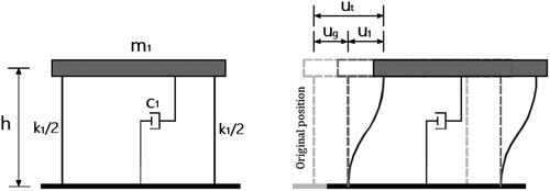
The structural stiffness and damping coefficients may be calculated using the following formulas (Abd-Elhamed, Shaban, & Mahmoud, 2018; Harris & Piersol, 2002) (1) $$k_1=\frac{4{\pi }^2{m}_1}{T_1^2}\text{and}{c}_1=2{\xi }_1\sqrt{k_1{m}_1},$$(1) where $T_1$ and $c_1$ stand for the natural period and damping ratio of the structural vibration, respectively.

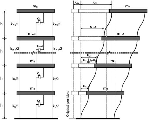
2.2. MDOF model

A planar base-excited shear frame building with $n$ degrees of freedom related to lateral displacements at each floor is taken into consideration to offer a more realistic work, as shown in Figure 2. At equally spaced narrative levels, the lumped masses $m_i\left(i=1,2,\cdots ,n\right)$ are dispersed. The parameters $k_i$ and $c_i$ stand for the $i\mathrm{th}$ floor’s stiffness and viscous damping coefficients, respectively.

Figure 2. Idealised MDOF mathematical model.

2.3. Earthquake modelling

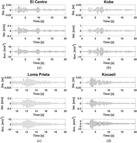
Table 1 lists a collection of four strong seismic-motion data, namely, El Centro (1940), Kobe (1995), Loma Prieta (1989), and Kocaeli (1999) (Abd-Elhamed et al., 2018). As seen in Table 1, four powerful ground movements with different peaks of ground acceleration (PGA) are shown. The earthquakes are estimated to have magnitudes ranging from 6.9 to 7.4 and site-source distances ranging from 0.6 to 43.4 km, where $M$ stands for magnitude and $D_{ss}$ for site-source distance. The time histories of acceleration for each earthquake are displayed in Figure 3.

Figure 3. Records of earthquake acceleration used for this study

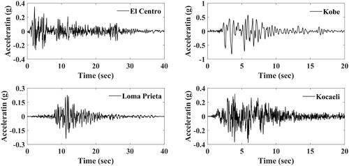
Table 1. Ground motion records used to excite building models (Abd-Elhamed et al., 2018).

Earthquake	Date	Station	PGA(g)	$M$	$D_{ss}$ (km)	Soil class
El Centro	18.05.1940	CA – Array Sta 9; Imperial Valley Irrigation District	0.341	6.9	12.2	D, C
Kobe	17.01.1995	0KJMA	0.8210	6.9	0.6	B, B
Loma Prieta	17.10.1989	Los Gatos, CA, NCJ066	0.19	6.9	43.4	B, NA
Kocaeli	17.08.1999	SKR SAKARYA	0.41	7.4	3	D, B

3. Mathematical formulation

In the next sections, the mathematical derivations of SDOF and MDOF models subjected to dynamic loads in terms of ground excitations are presented.

3.1. SDOF model

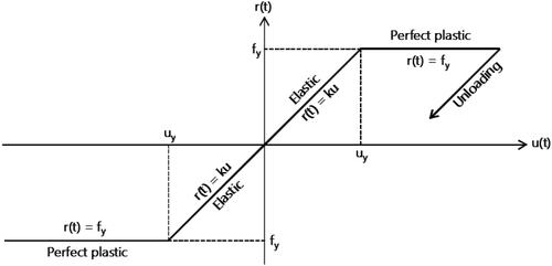
The displacement, $u_1\left(t\right),$ of the lumped mass, $m_1,$ specifies the movement of the system along a single route in the idealized SDOF model. According to Figure 4, the mathematical model is established by considering the various forces operating on $m_1$ such as inertia, $F_I(t),$ damping, $F_D(t),$ and resisting, $r_1\left(t\right),$ forces. Inevitably, the structure may respond nonlinearly and its dynamic response is in an inelastic (plastic) region. This phenomenon happens when the structure experiences abrupt and intense seismic stresses. As depicted in Figure 5, $r_1\left(t\right)$ equals $k_1{u}_1\left(t\right)$ or $\pm f_y$ in the elastic (linear state) or the plastic (nonlinear state) regions, respectively. The parameters $k_1$ and $f_y$ are the structural stiffness and the constant yield force for the structure, respectively. Thus, the SDOF’s resistive force may be stated as (2) $$r_1\left(t\right)=\delta k_1{u}_1\left(t\right)\pm \left(1-\delta \right)f_y,$$(2) where $\delta =\{\begin{array}{cc}1;& t\le t_y\\ 0;& t\ge t_y\end{array}$ and $t_y$ is the yield time at which $u_1\left(t\right)$ reaches its yield value.

Figure 4. Equilibrium of forces for SDOF model.

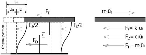
Figure 5. Idealized elastic-perfectly plastic behaviour.

The damping force is directly proportional to the lumped mass’s lateral velocity, ${\dot{u}}_1,$ and the damping coefficient, $c_1,$ of the dashpot so (3) $$F_D\left(t\right)=c_1{\dot{u}}_1\left(t\right).$$(3)

The mass of the model, $m_1;$ and its absolute acceleration, ${\ddot{u}}_t\left(t\right),$ are related to the inertial force as follows: (4) $$F_I\left(t\right)=m_1{\ddot{u}}_t\left(t\right)=m_1\left({\ddot{u}}_1\left(t\right)+{\ddot{u}}_g\left(t\right)\right).$$(4)

As a result, the idealized SDOF subjected to the ground excitation, ${\ddot{u}}_g\left(t\right),$ is nonlinearly modelled by (5) $$m_1{\ddot{u}}_1\left(t\right)+c_1{\dot{u}}_1\left(t\right)+r_1\left(t\right)=-{m_1\ddot{u}}_g\left(t\right).$$(5)

3.2. MDOF model

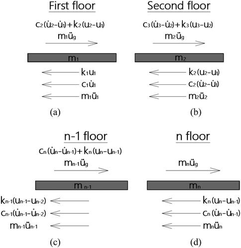
The MDOF lumped-mass structure’s equation of motion is derived by analyzing the equilibrium of forces at each lumped mass during earthquake excitation${\ddot{u}}_g\left(t\right).$ Figure 6 presents the applied external force on the first and the second floors as well as the induced internal forces due to equilibrium. After analyzing the 1st, 2nd, ${\left(n-1\right)}^{th},$ and $n^{th}$ floors by the same procedure illustrated in the idealized SDOF model, the equations of equilibrium are: (6) $$m_1{\ddot{u}}_1+c_1{\dot{u}}_1+r_1\left(t\right)-c_2\left({\dot{u}}_2{-\dot{u}}_1\right)-r_2\left(t\right)=-m_1{\ddot{u}}_g,$$(6) (7) $$m_2{\ddot{u}}_2+c_2\left({\dot{u}}_2{-\dot{u}}_1\right)+r_2\left(t\right)-c_3\left({\dot{u}}_3{-\dot{u}}_2\right)-r_3\left(t\right)=-m_2{\ddot{u}}_g,$$(7) (8) $$m_{n-1}{\ddot{u}}_{n-1}+c_{n-1}\left({\dot{u}}_{n-1}{-\dot{u}}_{n-2}\right)+r_{n-1}\left(t\right)-c_n\left({\dot{u}}_n{-\dot{u}}_{n-1}\right)-r_n\left(t\right)=-m_{n-1}{\ddot{u}}_g,$$(8) (9) $$m_n{\ddot{u}}_n+c_n\left({\dot{u}}_n{-\dot{u}}_{n-1}\right)+r_n\left(t\right)=-m_n{\ddot{u}}_g,$$(9) where the resisting force of MDOF $\left(n\ge 2\right)$ can take the form $r_n\left(t\right)=\delta k_n\left(u_n\left(t\right)-u_{n-1}\left(t\right)\right)\pm \left(1-\delta \right)f_y,\mathrm{}\delta =\{\begin{array}{cc}1;& t\le t_y\\ 0;& t\ge t_y\end{array}.$ The time $t_y$ is the yield one at which the displacement $u_n\left(t\right)-u_{n-1}\left(t\right)$ reaches its yield value. Hence, the equation of motion of MDOF building, subjected to base acceleration, can be expressed in a matrix form as follows: (10) $$\left(\begin{array}{ccccc}{m}_1& 0& \cdots & 0& 0\\ 0& m_2& \cdots & 0& 0\\ ⋮& ⋮& \ddots & ⋮& ⋮\\ 0& 0& \cdots & m_{n-1}& 0\\ 0& 0& \cdots & 0& m_n\end{array}\right)\left(\begin{array}{c}{\ddot{u}}_1\\ {\ddot{u}}_2\\ ⋮\\ {\ddot{u}}_{n-1}\\ {\ddot{u}}_n\end{array}\right)+\left(\begin{array}{ccccc}{c}_1+c_2& -c_2& \cdots & 0& 0\\ -c_2& c_2+c_3& \cdots & 0& 0\\ ⋮& ⋮& \ddots & ⋮& ⋮\\ 0& 0& \cdots & c_{n-1}+c_n& -c_n\\ 0& 0& \cdots & -c_n& c_n\end{array}\right)\left(\begin{array}{c}{\dot{u}}_1\\ {\dot{u}}_2\\ ⋮\\ {\dot{u}}_{n-1}\\ {\dot{u}}_n\end{array}\right)+\left(\begin{array}{c}{r}_1\\ r_2\\ ⋮\\ r_{n-1}\\ r_n\end{array}\right)=-\left(\begin{array}{c}{m}_1\\ m_2\\ ⋮\\ m_{n-1}\\ m_n\end{array}\right){\ddot{u}}_g,$$(10) where $u_i,$ ${\dot{u}}_i$ and ${\ddot{u}}_i\mathrm{}(i=1,2\dots ,n)$ denote displacements, velocities and accelerations for $i^{\mathrm{th}}$ storey, respectively.

4. Closed-form solutions

In order to obtain the closed-form solutions, the ground acceleration and the nonlinear term $\left(1-\delta \right)f_y,$ shown in Eq. (5)(5) $$m_1{\ddot{u}}_1\left(t\right)+c_1{\dot{u}}_1\left(t\right)+r_1\left(t\right)=-{m_1\ddot{u}}_g\left(t\right).$$(5) , are modelled using unit step functions $U\left(t-\tau \right)$ along subintervals of tiny length $\tau .$ Hence, they can be written in series forms using unit step functions as follows: (11) $$\begin{array}{c}{\ddot{u}}_g\left(t\right)=\sum _{i=1}^{\infty }{\ddot{u}}_g\left({\tau }_i\right)\left[U_i\left(t\right)-U_{i+1}\left(t\right)\right],\\ \left(1-\delta \right)f_y=\left(1-\delta \right)f_y\sum _{i=1}^{\infty }\left[U_i\left(t\right)-U_{i+1}\left(t\right)\right],\end{array}$$(11) where the unit step function is $U_i\left(t\right)=U\left(t-{\tau }_i\right)=\{\begin{array}{cc}1;& t\ge {\tau }_i\\ 0;& t<{\tau }_i\end{array}$ and ${\tau }_i=i\tau .$

Figure 6. (a) first, (b) second, (c) $n-1$ and (d) $n$ floors.

4.1. SDOF model

Inserting Eq. (11)(11) $$\begin{array}{c}{\ddot{u}}_g\left(t\right)=\sum _{i=1}^{\infty }{\ddot{u}}_g\left({\tau }_i\right)\left[U_i\left(t\right)-U_{i+1}\left(t\right)\right],\\ \left(1-\delta \right)f_y=\left(1-\delta \right)f_y\sum _{i=1}^{\infty }\left[U_i\left(t\right)-U_{i+1}\left(t\right)\right],\end{array}$$(11) into Eq. (5)(5) $$m_1{\ddot{u}}_1\left(t\right)+c_1{\dot{u}}_1\left(t\right)+r_1\left(t\right)=-{m_1\ddot{u}}_g\left(t\right).$$(5) leads to: (12) $$m_1{\ddot{u}}_1\left(t\right)+c_1{\dot{u}}_1\left(t\right)+\delta k_1{u}_1\left(t\right)=-m_1\sum _{i=1}^{\infty }{C}_{i1}\left[U_i\left(t\right)-U_{i+1}\left(t\right)\right],$$(12) where $C_{ij}={\ddot{u}}_g\left({\tau }_i\right)\pm \left(1-\delta \right)f_y/m_j.$

Knowing that the structure starts vibration from the rest and the initial velocity is zero makes the initial displacement and velocity as follows: (13) $$u_1\left(0\right)={\dot{u}}_1\left(0\right)=0.$$(13)

Applying Laplace transform on Eq. (12)(12) $$m_1{\ddot{u}}_1\left(t\right)+c_1{\dot{u}}_1\left(t\right)+\delta k_1{u}_1\left(t\right)=-m_1\sum _{i=1}^{\infty }{C}_{i1}\left[U_i\left(t\right)-U_{i+1}\left(t\right)\right],$$(12) subject to Eq. (13)(13) $$u_1\left(0\right)={\dot{u}}_1\left(0\right)=0.$$(13) and isolating $U_1\left(s\right)$ lead to: (14) $$U_1\left(s\right)=\frac{m_1}{m_1{s}^2+c_{1}s+\delta k_1}{G}_1\left(s\right),$$(14) where (15) $$G_j\left(s\right)=\sum _{i=1}^{\infty }{C}_{ij}\left[e^{-{\tau }_{i+1}s}-e^{-{\tau }_{i}s}\right],$$(15) and $s>0.$ Then, the closed-form solution of the deflection $u_1\left(t\right)$ is obtained after applying inverse Laplace transform on Eq. (15)(15) $$G_j\left(s\right)=\sum _{i=1}^{\infty }{C}_{ij}\left[e^{-{\tau }_{i+1}s}-e^{-{\tau }_{i}s}\right],$$(15) to get the exact solution: (16) $$u_1\left(t\right)=\frac{2m_1}{{\omega }_1}\sum _{i=1}^{\infty }{C}_{i1}\left[e^{-c_1\left(t-{\tau }_{i+1}\right)/2m_1}\sinh \left(\frac{{\omega }_1}{2m_1}\left(t-{\tau }_{i+1}\right)\right)U_{i+1}\left(t\right)-e^{-c_1\left(t-{\tau }_i\right)/2m_1}\sinh \left(\frac{{\omega }_1}{2m_1}\left(t-{\tau }_i\right)\right)U_i\left(t\right)\right],$$(16) where ${\omega }_1=\sqrt{c_1^2-4\delta k_1{m}_1}.$

4.2. MDOF model

In case of $n=2,$ knowing that the structure starts vibration from the rest makes the initial displacements and velocities as follows: (17) $$u_1\left(0\right)={\dot{u}}_1\left(0\right)=u_2\left(0\right)={\dot{u}}_2\left(0\right)=0.$$(17)

Substituting Eq. (11)(11) $$\begin{array}{c}{\ddot{u}}_g\left(t\right)=\sum _{i=1}^{\infty }{\ddot{u}}_g\left({\tau }_i\right)\left[U_i\left(t\right)-U_{i+1}\left(t\right)\right],\\ \left(1-\delta \right)f_y=\left(1-\delta \right)f_y\sum _{i=1}^{\infty }\left[U_i\left(t\right)-U_{i+1}\left(t\right)\right],\end{array}$$(11) into Eq. (10)(10) $$\left(\begin{array}{ccccc}{m}_1& 0& \cdots & 0& 0\\ 0& m_2& \cdots & 0& 0\\ ⋮& ⋮& \ddots & ⋮& ⋮\\ 0& 0& \cdots & m_{n-1}& 0\\ 0& 0& \cdots & 0& m_n\end{array}\right)\left(\begin{array}{c}{\ddot{u}}_1\\ {\ddot{u}}_2\\ ⋮\\ {\ddot{u}}_{n-1}\\ {\ddot{u}}_n\end{array}\right)+\left(\begin{array}{ccccc}{c}_1+c_2& -c_2& \cdots & 0& 0\\ -c_2& c_2+c_3& \cdots & 0& 0\\ ⋮& ⋮& \ddots & ⋮& ⋮\\ 0& 0& \cdots & c_{n-1}+c_n& -c_n\\ 0& 0& \cdots & -c_n& c_n\end{array}\right)\left(\begin{array}{c}{\dot{u}}_1\\ {\dot{u}}_2\\ ⋮\\ {\dot{u}}_{n-1}\\ {\dot{u}}_n\end{array}\right)+\left(\begin{array}{c}{r}_1\\ r_2\\ ⋮\\ r_{n-1}\\ r_n\end{array}\right)=-\left(\begin{array}{c}{m}_1\\ m_2\\ ⋮\\ m_{n-1}\\ m_n\end{array}\right){\ddot{u}}_g,$$(10) and applying Laplace transform on the resultant equation with the aid of Eq. (17)(17) $$u_1\left(0\right)={\dot{u}}_1\left(0\right)=u_2\left(0\right)={\dot{u}}_2\left(0\right)=0.$$(17) lead to: (18) $$\mathbf{AU}=\mathbf{B},$$(18) (19) $$\begin{array}{c}\mathbf{A}=\left(\begin{array}{cc}{\mathit{m}}_1{\mathit{s}}^2+\left({\mathit{c}}_1+{\mathit{c}}_2\right)\mathit{s}+\mathit{\delta }\left({\mathit{k}}_1+{\mathit{k}}_2\right)& -\left({\mathit{c}}_2\mathit{s}+\mathit{\delta }{\mathit{k}}_2\right)\\ -\left({\mathit{c}}_2\mathit{s}+\mathit{\delta }{\mathit{k}}_2\right)& {\mathit{m}}_2{\mathit{s}}^2+{\mathit{c}}_2\mathit{s}+\mathit{\delta }{\mathit{k}}_2\end{array}\right),\\ \mathbf{U}=\left(\begin{array}{c}{\mathit{U}}_1\left(\mathit{s}\right)\\ {\mathit{U}}_2\left(\mathit{s}\right)\end{array}\right),\mathbf{B}=\left(\begin{array}{c}{\mathit{m}}_1{\mathit{G}}_1\left(\mathit{s}\right)\\ {\mathit{m}}_2{\mathit{G}}_2\left(\mathit{s}\right)\end{array}\right).\end{array}$$(19)

The necessary condition for obtaining a unique solution for the system given in Eq. (18)(18) $$\mathbf{AU}=\mathbf{B},$$(18) is $\left|\mathit{A}\right|\ne 0$ which is satisfied. By using Cramer’s rule, the functions $U_j\left(s\right),$ $j=1,2,$ are given by: (20) $$U_j\left(s\right)=\frac{s^2+{\beta }_{j1}s+{\beta }_{j2}}{s^4+{\alpha }_1{s}^3+{\alpha }_2{s}^2+{\alpha }_{3}s+{\alpha }_4}{G}_j\left(s\right),$$(20) where (21) $$\begin{array}{c}{\beta }_{11}=\frac{c_2\left(m_1+m_2\right)}{m_1{m}_2},{\beta }_{21}=\frac{c_1}{m_1}+{\beta }_{11},{\beta }_{12}=\frac{\delta k_2\left(m_1+m_2\right)}{m_1{m}_2},\\ {\beta }_{22}=\frac{\delta k_1}{m_1}+{\beta }_{12},{\alpha }_1={\beta }_{21},{\alpha }_2=\frac{c_1{c}_2+\delta k_1{m}_1}{m_1{m}_2}+{\beta }_{12},\\ {\alpha }_3=\frac{\delta \left(c_1{k}_2+c_2{k}_1\right)}{m_1{m}_2},{\alpha }_4=\frac{{\delta }^2{k}_1{k}_2}{m_1{m}_2}.\end{array}$$(21)

Equation (20)(20) $$U_j\left(s\right)=\frac{s^2+{\beta }_{j1}s+{\beta }_{j2}}{s^4+{\alpha }_1{s}^3+{\alpha }_2{s}^2+{\alpha }_{3}s+{\alpha }_4}{G}_j\left(s\right),$$(20) is rewritten as follows: (22) $$U_j\left(s\right)=\left[\sum _{k=1}^2\frac{A_{jk}^{*}s+B_{jk}^{*}}{s^2+k_k^{*}s+h_k^{*}}\right]G_j\left(s\right),$$(22) where (23) $$\begin{array}{c}{A}_{jk}^{*}={\left(-1\right)}^k\frac{h_1^{*}{k}_2^{*}-k_1^{*}{h}_2^{*}+\left(h_2^{*}-h_1^{*}\right){\beta }_{j1}+\left(k_1^{*}-k_2^{*}\right){\beta }_{j2}}{{\left(h_1^{*}\right)}^2-\left(h_1^{*}+h_2^{*}\right)k_1^{*}{k}_2^{*}+h_1^{*}{\left(k_2^{*}\right)}^2-2h_1^{*}{h}_2^{*}+{\left(k_1^{*}\right)}^2{h}_2^{*}+{\left(h_2^{*}\right)}^2},\\ B_{jk}^{*}={\left(-1\right)}^j\frac{h_{3-k}^{*}\left(h_1^{*}-h_2^{*}\right)+\left(k_2^{*}-k_1^{*}\right)h_{3-k}^{*}{\beta }_{j1}+\left(h_2^{*}-h_1^{*}+k_{3-k}^{*}\left(k_1^{*}-k_2^{*}\right)\right){\beta }_{j2}}{{\left(h_1^{*}\right)}^2-\left(h_1^{*}+h_2^{*}\right)k_1^{*}{k}_2^{*}+h_1^{*}{\left(k_2^{*}\right)}^2-2h_1^{*}{h}_2^{*}+{\left(k_1^{*}\right)}^2{h}_2^{*}+{\left(h_2^{*}\right)}^2},\\ k_k^{*}=\frac{1}{2}{\alpha }_1+{\left(-1\right)}^{k}a,h_k^{*}=\lambda +{\left(-1\right)}^{k}b,k=1,2,\\ a=\frac{1}{2}\sqrt{8\lambda +{\alpha }_1^2-4{\alpha }_2},b=\sqrt{{\lambda }^2-{\alpha }_4},ab=\frac{1}{2}\left({\alpha }_1\lambda -{\alpha }_3\right),\\ \lambda =\frac{1}{6}\left({\alpha }_2-\sqrt[3]{2}{\left(-{\omega }_3+\sqrt{{\omega }_3^2-4{\omega }_2^3}\right)}^{-1/3}-\frac{1}{\sqrt[3]{2}}{\left(-{\omega }_3+\sqrt{{\omega }_3^2-4{\omega }_2^3}\right)}^{1/3}\right),\\ {\omega }_2={\alpha }_2^2-3{\alpha }_1{\alpha }_3+12{\alpha }_4,{\omega }_3=2{\alpha }_2^3-9{\alpha }_2\left({\alpha }_1{\alpha }_3+8{\alpha }_4\right)+27\left({\alpha }_3^2+{\alpha }_1^2{\alpha }_4\right).\end{array}$$(23)

By applying inverse Laplace transform on Eq. (22)(22) $$U_j\left(s\right)=\left[\sum _{k=1}^2\frac{A_{jk}^{*}s+B_{jk}^{*}}{s^2+k_k^{*}s+h_k^{*}}\right]G_j\left(s\right),$$(22) , the closed form solution is as follows: (24) $$u_j\left(t\right)=\sum _{i=1}^{\infty }{C}_{ij}\left[\sum _{k=1}^2\left[e^{-k_k^{*}t/2}\left[e^{k_k^{*}{\tau }_{i+1}/2}\left[f_{jk}\left(t-{\tau }_{i+1}\right)+g_{jk}\left(t-{\tau }_{i+1}\right)\right]U_{i+1}\left(t\right)-e^{k_k^{*}{\tau }_i/2}\left[f_{jk}\left(t-{\tau }_i\right)+g_{jk}\left(t-{\tau }_i\right)\right]U_i\left(t\right)\right]\right]\right],$$(24) where (25) $$\begin{array}{c}{f}_{jk}\left(T\right)=A_{jk}^{*}\cosh \left(b_{k}T\right),g_{jk}\left(T\right)=\frac{a_{jk}}{2b_k}\sinh \left(b_{k}T\right),\\ a_{jk}=2B_{jk}^{*}-k_k^{*}{A}_{jk}^{*},b_k=\frac{1}{2}\sqrt{{\left(k_k^{*}\right)}^2-4h_k^{*}},\end{array}$$(25) $T$ is a dummy variable, $j=1,2$ and $k=1,2.$

In case of $n>2,$ knowing that the structure starts vibration from the rest makes the initial displacements and velocities as follows: (26) $$u_1\left(0\right)={\dot{u}}_1\left(0\right)=u_2\left(0\right)={\dot{u}}_2\left(0\right)=\cdots =u_n\left(0\right)={\dot{u}}_n\left(0\right)=0.$$(26)

Substituting Eq. (11)(11) $$\begin{array}{c}{\ddot{u}}_g\left(t\right)=\sum _{i=1}^{\infty }{\ddot{u}}_g\left({\tau }_i\right)\left[U_i\left(t\right)-U_{i+1}\left(t\right)\right],\\ \left(1-\delta \right)f_y=\left(1-\delta \right)f_y\sum _{i=1}^{\infty }\left[U_i\left(t\right)-U_{i+1}\left(t\right)\right],\end{array}$$(11) into Eq. (10)(10) $$\left(\begin{array}{ccccc}{m}_1& 0& \cdots & 0& 0\\ 0& m_2& \cdots & 0& 0\\ ⋮& ⋮& \ddots & ⋮& ⋮\\ 0& 0& \cdots & m_{n-1}& 0\\ 0& 0& \cdots & 0& m_n\end{array}\right)\left(\begin{array}{c}{\ddot{u}}_1\\ {\ddot{u}}_2\\ ⋮\\ {\ddot{u}}_{n-1}\\ {\ddot{u}}_n\end{array}\right)+\left(\begin{array}{ccccc}{c}_1+c_2& -c_2& \cdots & 0& 0\\ -c_2& c_2+c_3& \cdots & 0& 0\\ ⋮& ⋮& \ddots & ⋮& ⋮\\ 0& 0& \cdots & c_{n-1}+c_n& -c_n\\ 0& 0& \cdots & -c_n& c_n\end{array}\right)\left(\begin{array}{c}{\dot{u}}_1\\ {\dot{u}}_2\\ ⋮\\ {\dot{u}}_{n-1}\\ {\dot{u}}_n\end{array}\right)+\left(\begin{array}{c}{r}_1\\ r_2\\ ⋮\\ r_{n-1}\\ r_n\end{array}\right)=-\left(\begin{array}{c}{m}_1\\ m_2\\ ⋮\\ m_{n-1}\\ m_n\end{array}\right){\ddot{u}}_g,$$(10) and applying Laplace transform on the resultant equation with the aid of Eq. (26)(26) $$u_1\left(0\right)={\dot{u}}_1\left(0\right)=u_2\left(0\right)={\dot{u}}_2\left(0\right)=\cdots =u_n\left(0\right)={\dot{u}}_n\left(0\right)=0.$$(26) , lead to the form of Eq. (18)(18) $$\mathbf{AU}=\mathbf{B},$$(18) whose unknowns are the functions $U_j\left(s\right),$ $j=1,2,\cdots ,n,$ given by: (27) $$U_j\left(s\right)=\left[\left(s^{2n-2}+\sum _{k=1}^{2n-2}{\beta }_{jk}{s}^{2n-2-k}\right)/\left(s^{2n}+\sum _{k=1}^{2n}{\alpha }_k{s}^{2n-k}\right)\right]G_j\left(s\right),$$(27) which is rewritten in the form: (28) $$U_j\left(s\right)=\left[\sum _{k=1}^n\frac{A_{jk}^{*}s+B_{jk}^{*}}{s^2+k_k^{*}s+h_k^{*}}\right]G_j\left(s\right).$$(28)

Similar to the procedure given in the two-DOF building model, the closed-from solution is (29) $$u_j\left(t\right)=\sum _{i=1}^{\infty }{C}_{ij}\left[\sum _{k=1}^n\left[e^{-k_k^{*}t/2}\left[e^{k_k^{*}{\tau }_{i+1}/2}\left[f_{jk}\left(t-{\tau }_{i+1}\right)+g_{jk}\left(t-{\tau }_{i+1}\right)\right]U_{i+1}\left(t\right)-e^{k_k^{*}{\tau }_i/2}\left[f_{jk}\left(t-{\tau }_i\right)+g_{jk}\left(t-{\tau }_i\right)\right]U_i\left(t\right)\right]\right]\right],$$(29) after producing the suitable formulas of ${\alpha }_k,$ ${\beta }_{jk},$ $a,$ $b,$ $\lambda ,$ $A_{jn}^{*},$ $B_{jn}^{*},$ $k_n^{*}$ and $h_n^{*}$ and using the formulas given in Eq. (25)(25) $$\begin{array}{c}{f}_{jk}\left(T\right)=A_{jk}^{*}\cosh \left(b_{k}T\right),g_{jk}\left(T\right)=\frac{a_{jk}}{2b_k}\sinh \left(b_{k}T\right),\\ a_{jk}=2B_{jk}^{*}-k_k^{*}{A}_{jk}^{*},b_k=\frac{1}{2}\sqrt{{\left(k_k^{*}\right)}^2-4h_k^{*}},\end{array}$$(25) where $j=1,2,\cdots ,n$ and $k=1,2,\cdots ,n.$

5. Results

With the use of Laplace transform, an analytical formulation of Eq. (16)(16) $$u_1\left(t\right)=\frac{2m_1}{{\omega }_1}\sum _{i=1}^{\infty }{C}_{i1}\left[e^{-c_1\left(t-{\tau }_{i+1}\right)/2m_1}\sinh \left(\frac{{\omega }_1}{2m_1}\left(t-{\tau }_{i+1}\right)\right)U_{i+1}\left(t\right)-e^{-c_1\left(t-{\tau }_i\right)/2m_1}\sinh \left(\frac{{\omega }_1}{2m_1}\left(t-{\tau }_i\right)\right)U_i\left(t\right)\right],$$(16) provided a precise solution to the dynamic equation of motion of the seismically triggered one-story shear building model illustrated in Figure 1 and subjected to the initial circumstances given in Eq. (13)(13) $$u_1\left(0\right)={\dot{u}}_1\left(0\right)=0.$$(13) . The dynamic equations of motion for the $n$-DOF construction mode system depicted in Figure 2 is similarly solved analytically and then expressed in Eq. (29)(29) $$u_j\left(t\right)=\sum _{i=1}^{\infty }{C}_{ij}\left[\sum _{k=1}^n\left[e^{-k_k^{*}t/2}\left[e^{k_k^{*}{\tau }_{i+1}/2}\left[f_{jk}\left(t-{\tau }_{i+1}\right)+g_{jk}\left(t-{\tau }_{i+1}\right)\right]U_{i+1}\left(t\right)-e^{k_k^{*}{\tau }_i/2}\left[f_{jk}\left(t-{\tau }_i\right)+g_{jk}\left(t-{\tau }_i\right)\right]U_i\left(t\right)\right]\right]\right],$$(29) . This study results in the form of structural responses are compared with precise numerical outcomes generated by Newmark’s step-by-step iteration approach via a built-in MATLAB code to confirm the accuracy of derived analytical formulations.

5.1. SDOF model

In the performed analysis, the mass, stiffness, and damping coefficient for a single-story building are assumed as $m_1=30\times {10}^3\mathrm{}\mathrm{kg},$ $k_1=1.3159\times {10}^7\mathrm{}\mathrm{N}/\mathrm{m},$ and $c_1={6.2832\times 10}^4\mathrm{kg}/\mathrm{s},$ respectively. The SDOF building model is analysed using four-ground motion records, as shown in Table 1, with varied peak ground accelerations. The comparison between the analytical and numerical results in terms of peak values of displacement, velocity, and acceleration response quantities is shown in Table 2.

Table 2. Peak structural response quantities SDOF building model.

Earthquake	Newmark’s method			Exact solutions			% Error
	$u_{\mathit{Newmark}}$	${\dot{u}}_{\mathit{Newmark}}$	${\ddot{u}}_{\mathit{Newmark}}$	$u_{\mathit{Exact}}$	${\dot{u}}_{\mathit{Exact}}$	${\ddot{u}}_{\mathit{Exact}}$	$u$	$\dot{u}$	$\ddot{u}$
El Centro	0.0158	0.3317	8.9537	0.0158	0.3328	9.0624	0.00	0.33	1.20
Kobe	0.0415	0.6798	12.6686	0.0419	0.6977	12.945	0.95	2.57	2.14
LomaPrieta	0.0239	0.4578	9.1851	0.0238	0.4593	9.248	0.42	0.33	0.68
Kocaeli	0.0191	0.4057	11.301	0.0192	0.4088	11.308	0.52	0.76	0.06

$u$ = peak displacement [m], $\dot{u}$= peak velocity [m/s], $\ddot{u}$= peak acceleration [m/s²]

Table 2 clearly shows that Eq. (16)(16) $$u_1\left(t\right)=\frac{2m_1}{{\omega }_1}\sum _{i=1}^{\infty }{C}_{i1}\left[e^{-c_1\left(t-{\tau }_{i+1}\right)/2m_1}\sinh \left(\frac{{\omega }_1}{2m_1}\left(t-{\tau }_{i+1}\right)\right)U_{i+1}\left(t\right)-e^{-c_1\left(t-{\tau }_i\right)/2m_1}\sinh \left(\frac{{\omega }_1}{2m_1}\left(t-{\tau }_i\right)\right)U_i\left(t\right)\right],$$(16) makes a very good prediction of the response characteristics for the SDOF building.

Additionally, the findings show that the percentage differences between the analytical and numerical results were estimated to be less than 3%. The time-history responses of the excited SDOF building model that were generated from a closed-form solution to the Kobe, El Centro, Loma Prieta, and Kocaeli earthquakes are shown in Figure 7 in the appropriate order.

Figure 7. Induced displacement, velocity and acceleration time-histories of the SDOF system with respect to the (a) El Centro, (b) Kobe, (c) Loma Prieta and (d) Kocaeli records.

5.2. MDOF model

To validate the reliability of the proposed analytical method to predict the seismic responses of multi-storey frame buildings, the three-story building modelled as an MDOF system as shown in Figure 2 is considered for this purpose. This building model has a uniform storey height $h=3\mathrm{m}.$ Undamped natural frequencies of the MDOF building structure are ${\tilde{\omega }}_1=5.32$rad/s, ${\tilde{\omega }}_2=13.60$rad/s, and ${\tilde{\omega }}_3=19.48$rad/s. The fundamental mode shape normalized by the modal coordinate of the load mass $m_1$ is computed as ${\varphi }_1={\left\{0.4330.7951.000\right\}}^T.$

According to Eq. (30)(30) $$c_j=\frac{2{\zeta }_1}{{\tilde{\omega }}_j}{k}_j\left(j=1,2,3\right),$$(30) , the damping coefficients of the examined structure are supposed to be proportional to the stiffness (classically damped system), i.e. (30) $$c_j=\frac{2{\zeta }_1}{{\tilde{\omega }}_j}{k}_j\left(j=1,2,3\right),$$(30) where ${\zeta }_1$ is the fundamental mode shape’ damping ratio (taken equal to 2%).

The inertial and elastic properties of the structure are given in Table 3. Whereas the peak responses at each storey level as determined by Newmark’s method and the proposed approach are listed in Table 4. The superior capacity of the proposed technique to produce extremely accurate results, even for multi-story structures, is demonstrated by the outstanding agreement between the closed-form results and the numerical findings.

Table 3. Inertial and elastic properties of the 3-DOF structure.

$i$	$m_i$ [kg]	$k_i$ [$\frac{\mathrm{N}}{\mathrm{m}}$]	$c_i$ [$\frac{\mathrm{N}.\mathrm{s}}{\mathrm{m}}$]
1	$30\times {10}^3$	$3.46\times {10}^6$	26000
2	$25\times {10}^3$	$0.9\times 3.46\times {10}^6$	23400
3	$20\times {10}^3$	$0.8\times 3.46\times {10}^6$	20800

Table 4. Peak structural response quantities three-DOF building model.

Earthquake	Newmark iteration method			Exact solutions			% Error
	$u_{\mathit{Newmark}}$	${\dot{u}}_{\mathit{Newmark}}$	${\ddot{u}}_{\mathit{Newmark}}$	$u_{\mathit{Exact}}$	${\dot{u}}_{\mathit{Exact}}$	${\ddot{u}}_{\mathit{Exact}}$	$u$	$\dot{u}$	$\ddot{u}$
1st storey
El Centro	0.0658	0.477	4.2134	0.0664	0.4592	4.2924	0.90	3.88	1.84
Kobe	0.1681	1.362	11.9236	0.1679	1.3903	11.9025	0.12	2.04	0.18
Loma Prieta	0.0454	0.3598	4.9231	0.0462	0.3638	4.8946	1.73	1.10	0.58
Kocaeli	0.0691	0.3797	5.1292	0.0694	0.3888	5.1601	0.43	2.34	0.60
2nd storey
El Centro	0.1188	0.6824	5.0637	0.1199	0.7041	5.0608	0.92	3.08	0.06
Kobe	0.3225	2.1483	13.7969	0.3301	2.1152	13.9508	2.30	1.56	1.10
Loma Prieta	0.0702	0.4179	3.8065	0.0710	0.4277	3.8557	1.13	2.29	1.28
Kocaeli	0.1233	0.6655	4.9226	0.1260	0.6865	4.9592	2.14	3.06	0.74
3rd storey
El Centro	0.1552	0.8069	7.2661	0.1570	0.8102	7.4451	1.15	0.41	2.40
Kobe	0.4600	3.1066	22.7379	0.4651	3.1376	22.9682	1.10	0.99	1.00
Loma Prieta	0.1033	0.5752	5.8431	0.1025	0.5886	5.8705	0.78	2.28	0.47
Kocaeli	0.1502	0.8747	5.6486	0.1535	0.8936	5.5755	2.15	2.12	1.31

$u$ = peak displacement [m], $\dot{u}$= peak velocity [m/s], $\ddot{u}$= peak acceleration [m/s²]

Additionally, as shown in Table 4, the biggest percentage difference between analytical and numerical findings was determined to be less than 4%, demonstrating that the suggested technique can properly forecast seismic reactions of buildings. As a result of the El Centro, Kobe, Loma Prieta, and Kocaeli earthquake records, the displacement, velocity, and acceleration time histories of the considered MDOF building are displayed in Figures 8–11, respectively.

Figure 8. Induced displacement, velocity and acceleration time-histories for first, second, and third storey of MDOF system with respect to the El Centro earthquake.

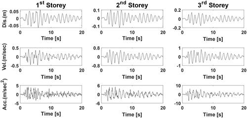
Figure 9. Induced displacement, velocity and acceleration time-histories for first, second, and third storey of MDOF system with respect to the Kobe earthquake.

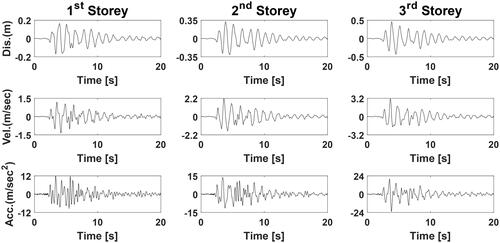
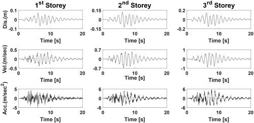
Figure 10. Induced displacement, velocity and acceleration time-histories for first, second, and third storey of MDOF system with respect to the Loma Prieta earthquake.

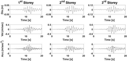
Figure 11. Induced displacement, velocity and acceleration time-histories for first, second, and third storey of MDOF system with respect to the Kocaeli earthquake.

6. Conclusion

In the current research, a closed-form analytical solution for the dynamic equations of motion of SDOF and MDOF seismically excited models are obtained using the Laplace transform. Using the Newmark numerical approach, the response quantities of interest in terms of the induced displacement, velocity, and acceleration have been determined and compared to the exact solutions. The findings of the deduced closed-form solutions and the associated numerical results are found to be in good agreement. Therefore, it is safe to apply the suggested closed-form solution to capture the reactions of seismically stimulated structures.

Disclosure statement

No potential conflict of interest was reported by the authors.

References

- Abd-Elhamed, A., & Mahmoud, S. (2019a). Simulation analysis of TMD controlled building subjected to far- and near-fault records considering soil-structure interaction. Journal of Building Engineering, 26, 100930. doi:10.1016/j.jobe.2019.100930
- Abd-Elhamed, A., & Mahmoud, S. (2019b). Seismic response evaluation of structures on improved liquefiable soil. European Journal of Environmental and Civil Engineering, 25, 1695–1717. doi:10.1080/19648189.2019.1595738
- Abd-Elhamed, A., & Tolan, M. (2022). Tuned liquid damper for vibration mitigation of seismic-excited structures on soft soil. Alexandria Engineering Journal, 61(12), 9583–9599. doi:10.1016/j.aej.2022.03.051
- Abd-Elhamed, A., Shaban, Y., & Mahmoud, S. (2018). Predicting dynamic response of structures under earthquake loads using logical analysis of data. Buildings, 8(4), 61. doi:10.3390/buildings8040061
- Ayoub, S., & Reza, E. (2022). A framework for exergy analysis of process control systems. Journal of Process Control, 109, 104–119.
- Bathe, K. J. (1996). Finite element procedures. Hoboken, NJ: Prentice-Hall, Inc.
- Carnahan, B., Lither, H. A., & Wilkes, J. O. (1969). Applied numerical methods. Wiley, New York.
- Castanon, L. J., Naredo, J. L., Zuluaga, J. R., Banuelos-Cabral, E., & Pablo, G. (2021). Laplace transform inversion through the theta algorithm for power-system EMT analysis. Electric Power Systems Research, 197, 107342. doi:10.1016/j.epsr.2021.107342
- Castaldo, P., & Tubaldi, E. (2018). Influence of ground motion characteristics on the optimal single concave sliding bearing properties for base-isolated structures. Soil Dynamics and Earthquake Engineering, 104, 346–364. doi:10.1016/j.soildyn.2017.09.025
- Chopra, A. (2007). Dynamics of structures: Theory and applications to earthquake engineering (3rd ed.). Upper Saddle River, NJ: Prentice-Hall.
- Christian, C., & Frank, R. (2021). Comparison of implicit and explicit numerical integration schemes for a bounding surface soil model without elastic range. Computers and Geotechnics, 140. doi:10.1016/j.compgeo.2021.104206.
- Dukkipati, R. V. (2010). Numerical methods. New Age International (P) Ltd., Publishers, New Delhi.
- El-Azab, M. S., Mahmoud, S., & Abd-Elhameed, A. (2011). Seismic response evaluation of buildings considering soil flexibility. Advanced Materials Research, 243, 1383–1390.
- Gangadharaiah, Y., & Sandeep, N. (2021). Engineering applications of the laplace transform. Cambridge Scholars Publishing, Cambridge.
- Geradin, M., & Rixen, D. (1997). Mechanical vibrations-theory and application to structural dynamics (2nd ed.). Wiley, New York.
- Hairer, E., & Wanner, G. (1991). Solving ordinary differential equations II, Vol. 14: Stiff and differential-algebraic problems. Berlin, Springer-Verlag, 614 p. doi:10.1007/978-3-642-05221-7
- Hareen, C. B., & Mohan, S. (2021). Evaluation of seismic torsional response of ductile RC buildings with soft first story. Structures, 29, 1640–1654. doi:10.1016/j.istruc.2020.12.031
- Harris, C. M., & Piersol, A. G. (2002). Harris’ shock and vibration handbook (ed. C. M. Harris & A. G. Piersol). McGraw-Hill Publishing, New York.
- He, J., Amer, T., Abolila, A., & Galal, A. (2022). Stability of three degrees-of-freedom auto-parametric system. Alexandria Engineering Journal, 61(11), 8393–8415. doi:10.1016/j.aej.2022.01.064
- He, C. H., Amer, T. S., Tian, D., Abolila, A. F., & Galal, A. A. (2022). Controlling the kinematics of a spring-pendulum system using an energy harvesting device. Journal of Low Frequency Noise, 0(0), 1–24. doi:10.1177/14613484221077474
- Huang, L.,Deng, L.,Li, A.,Gao, R.,Zhang, L., &Lei, W. (2021). A novel approach for solar greenhouse air temperature and heating load prediction based on Laplace transform. Journal of Building Engineering, 44, 102682 10.1016/j.jobe.2021.102682.
- Hussain, M. A., & Dutta, S. C. (2020). Inelastic seismic behaviour of asymmetric structures under bidirectional ground motion: An effort to incorporate the effect of bidirectional interaction in load resisting elements. Structures, 25, 241–255. doi:10.1016/j.istruc.2020.03.014
- James, G. (1966). Holbrook, Laplace transforms for electronic engineers (2nd ed.). Elsevier Science & Technology.
- Jia, J., Song, N., Xu, Z., He, Z., & Bai, Y. (2015). Structural damage distribution induced by Wenchuan Earthquake on 12th May, 2008. Earthquakes and Structures, 9(1), 93–109. doi:10.12989/eas.2015.9.1.093
- Joel Schiff, L. (1999). The Laplace transform: Theory and applications.
- Linus, W., Illias, H., & Arno, S. (2022). Scenario-based robustness assessment of building system life cycle performance. Applied Energy, 311. doi:10.1016/j.apenergy.2022.118606
- Mahmoud, S., Abd-Elhameed, A., & Jankowski, R. (2012). Behaviour of colliding multi-storey buildings under earthquake excitation considering soil-structure interaction. Applied Mechanics and Materials, 166, 2283–2292.
- Martí, L., & Daichao, S. (2022). Assessing the accuracy and efficiency of different order implicit and explicit integration schemes. Computers and Geotechnics, 141. doi:10.1016/j.compgeo.2021.104531
- Osama, H., & Huda, A. (2018). Computational methods based Laplace decomposition for solving nonlinear system of fractional order differential equations. Alexandria Engineering Journal, 57(4), 3549–3557. doi:10.1016/j.aej.2017.11.020
- Paz, M. (1997). Structural dynamics: Theory and computation (4th ed.). Chapman & Hall, New York.
- Rajasekaran, S. (2009). 7—Dynamic response of structures using numerical methods. In Woodhead publishing series in civil and structural engineering, structural dynamics of earthquake engineering (pp. 171–239). Woodhead Publishing, Cambridge, UK. doi:10.1533/9781845695736.1.171
- Sawant, L. S. (2018). Applications of Laplace transform in engineering fields. International Research Journal of Engineering and Technology (IRJET), 5(5), 3100–3105.
- Söderlind, G. (2006). Time-step selection algorithms: Adaptivity, control, and signal processing. Applied Numerical Mathematics, 56(3–4), 488–502. doi:10.1016/j.apnum.2005.04.026
- Xinpeng, L., & Xianqiang, Y. (2020). A variational Bayesian approach for robust identification of linear parameter varying systems using mixture Laplace distributions. Neurocomputing, 395(2020), 15–23. doi:10.1016/j.neucom.2020.01.088
- Yang, X.-S. (2016). Engineering mathematics with examples and applications. Academic Press, London.