Obtaining and Applying Public Data for Training Students in Technical Statistical Writing: Case Studies with Data from U.S. Geological Survey and General Ecological Literature

Abstract

Effective undergraduate statistical education requires training using real-world data. Textbook datasets seldom match the complexities and messiness of real-world data and finding these datasets can be challenging for educators. Consulting and industrial datasets often have nondisclosure agreements. Academic datasets often require subject area expertise beyond those of a general education or lack connections to real-world applications. Many governments, including the United States, now require the release of data from projects they directly complete or fund though grants and contracts. We show how statistical educators may find datasets and incorporate them into courses. Specifically, we use two examples from the U.S. Geological Survey (USGS) and one example from the ecology literature. We demonstrate the use of these datasets in an upper-level analysis of variance (ANOVA) class. In addition to describing how we found the datasets, we describe how to include them into course work and the course’s student assessments. We have used these datasets over multiple semesters and included student feedback from these courses. Although our examples focus on an ANOVA class, the general methods for finding data shared here could be used for statistical classes ranging from high school to graduate education. Supplementary materials for this article are available online.

Keywords:

• Earth science data
• Environmental data
• Forensic statistics
• Government data
• Undergraduate education

1 Introduction

Effective and relevant undergraduate statistics programs require explicit and repeated training and experiences with statistical communication, data wrangling, and the broad statistical modeling process. The American Statistical Association (ASA) formally recognized this as part of their Curriculum Guidelines for Undergraduate Programs in Statistical Science (2014). These guidelines highlight the importance of both developing the ability to communicate and the incorporation of real applications specifically involving the analysis of non-textbook, messy data into statistical education. These guidelines recognize four key components for statistical education: (a) the importance of data science, (b) the use of real applications of statistics to data, (c) the need for more diverse models and approaches, and (d) the ability to communicate about data and statistical model results.

As part of this process, professors and others teaching undergraduate statistics bring data into their classroom. Traditionally, most example datasets found in textbooks usually contain “tidy” data (see Wickham (2014) for a definition and discussion on “tidy” data), that may or may not be real-word data, and often clearly lend themselves to one type of analysis with minimal modeling choices (Engel 2017). These datasets allow the teachers to focus on teaching specific statistical methods, which may be appropriate in many settings. But, common “textbook” datasets, by definition, are usually commonly used examples. Thus, students may have seen datasets before or be able to easily search for existing analysis approaches for the data either using internet search engines or software help files (e.g., searching R software’s documentation or dependencies for uses of datasets). Lastly, using textbook datasets does not often allow students to see the challenges of real-world data collection and generation (textbooks often present clean data “as is” rather than describing and including discussion on the subject area creation process for data), nor the work required to generate data coupled with the often-inherent messiness of real-world data (Engel 2017; Wickham 2014). Hence, the ASA’s 2014 guidelines to address these shortcomings.

Thus, statistical educators may want to find new datasets for their courses. However, finding new datasets can be difficult. Consulting and industrial data often have nondisclosure clauses due to proprietary data (e.g., see Deming 1972 for an example statistical consulting contract in the peer reviewed literature or private discussions on the ASA’s Statistical Consulting Section forum for more recent examples). Many academic research datasets require prerequisite knowledge beyond a general college education and lack intuition (e.g., Lanie et al. 2004) or may not be applicable to broad, real-world settings (Bozeman and Boardman 2009). For example, we have used astronomy and psychology data during previous semesters, but found these datasets to require expertise beyond what could be easily covered in a short lecture. In contrast, the biology and ecology datasets we found could readily be understood by undergraduates using their intuition of the study systems. Other easily understandable datasets, such as biomedical data, can be restricted due to patient privacy concerns (Malin, Emam, and O’Keefe 2013).

This collaboration between a government research agency, the U.S. Geological Survey (USGS), and a comprehensive research university, the University of Wisconsin – La Crosse (UWL), helps to overcome many challenges in finding new data for classroom examples. Here, we share about our successes and challenges in using public data and associated published research papers drawn primarily from the USGS to support these curricular goals at UWL. This partnership helps UWL train their students using approaches currently used by natural resource managers and helps USGS to promote their data and train future statisticians and scientists for potential positions in the federal government and other agencies (see Erickson et al. 2021 for examples of current quantitative needs in natural resource management). Furthermore, the OPEN Government Data Act (2007) requires the USGS to share data, something USGS does using a lifecycle model to maintain and disseminate data (Faundeen et al. 2014; Faundeen and Hutchison 2017).

Herein, we first describe the pedagogical goals, academic context, and structure of the courses included in our study. Next, we describe how we set up the essential components for applying data to coursework, specifically data sources; required student tools; student tasks and projects; and assessments. Then, we present three case studies including assessments with round goby (Neogobius melanostomus) data, sea lamprey (Petromyzon marinus) data, and grass disease (barley and cereal yellow dwarf viruses) data.

2 Pedological Goals and Academic Context

Practicing statisticians require skills not always taught in traditional education programs, hence, the ASA’s 2014 report (American Statistical Association 2014). First, practicing statisticians require communication skills (both verbal and written) to complement their statistical and analytics work. Second, practicing statisticians work with real world, messy data. Wickham (2014) describes the theory behind “tidy” data and describes how most datasets are inherently messy unless conscious effort goes into tidying the data. Often, practicing statisticians spend a large portion of their time cleaning and formatting data prior to analysis.

Both communicating and working with real world data are hands-on experiences that cannot, based upon our experiences, be done theoretically. Hence, educators who give their students the opportunity to work with and communicate statistical model results using real-world data are giving them a valuable and rare learning experience that enhances their education. An additional benefit of using real-world datasets is that students often can relate to the datasets in a way that is not possible with textbook datasets. For example, our case studies relate directly to environmental problems in the Great Lakes, Wisconsin, and the Mississippi River basin and many students enjoy outdoor recreational activities that can be negatively impacted by aquatic invasive species).

The natural resource example datasets also fit into the general purpose of our institution. At UWL, undergraduate statistics majors have a broad statistical education that includes a wide base of courses such as general mathematics, mathematical and theoretical statistics, and computer science as well as upper level, applied statistical courses. These upper-level courses help give students the tools necessary to start their statistical careers. These are formalized through Student Learning Outcomes (SLOs; Text box 1) at UWL.

Textbox 1. Statistics program student learning outcomes (SLOs) for UWL’s undergraduate statistics major program.

Students completing this program will be able to:

1. apply appropriate statistical methods for a variety of data analysis situations

2. conduct the computational aspects for a variety of statistical procedures using statistical software, including packaged functions, data manipulation and management, and simulation.

3. effectively communicate statistical analyses orally and in writing

4. explain distribution theory and how it relates to the construction of statistical inference procedures like confidence intervals and hypothesis tests

We have used the datasets described in this article and similar datasets in multiple courses. However, we are specifically reporting results from the “Analysis of Variance (ANOVA) and Design of Experiments” course. The course is primarily for statistics majors, although advanced non-majors, statistics minors, and Master’s of Science students from other departments regularly take the course. The course covers the basics of ANOVA and necessary data collection and study design for the application of ANOVA as an analysis tool. The course requires either successful completion of a calculus-based probability and statistics course (200-level) or an introductory statistics course in addition to an applied statistical methods course (100-level + 300-level). All students entering the course should have at least a modest amount of experience using statistical software like R or SPSS. Even with these course pre-requisites in place, there is generally a broad range of student experience and skills at the outset of the course.

3 Essential Components

3.1 Data Sources

The U.S. Government maintains data catalogues for federal and voluntary nonfederal public data. These data catalogues exist following organization hierarchy and also link to a data warehouse (Figure 1). At the top of this hierarchy is data.gov, which is run by the U.S. General Services Administration. Departments, such as the U.S. Department of the Interior, host their own data catalogues, such as data.doi.gov. Within the Department of Interior, the USGS hosts their own data catalogue, data.usgs.gov. In turn, most USGS datasets are hosted (synonymously stored, posted, or warehoused) on ScienceBase.gov. Likewise, other departments have similar structures such as the U.S. Department of Commerce (https://data.commerce.gov/) that hosts agency data from both the U.S. Census Bureau (https://data.census.gov/) and the National Oceanic and Atmospheric Administration (https://data.noaa.gov/).

Fig. 1 Example of data catalogue hierarchy and linkages to a data warehouses. In this figure, arrows represent how data catalogues pull information for other sources. For example, data.gov pulls information from data.doi.gov. In theory, all data in data.doi.gov should be pulled to data.gov. However, due to database and metadata challenges, all datasets linked in one database do not always link to higher levels.

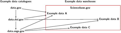
Challenges exist using both the data catalogues and data referenced by them. First, the data catalogues do not always communicate correctly with each other. Thus, data may be “hiding” at lower levels and not visible to higher catalogues. Second, data file formats vary across agencies and people. As a general observation, using a search filter for “csv” or similar data structures often helped us to sort through data to find easier to use datasets because we found these datasets to usually be easy to work with. However, the previously mentioned challenges with the data catalogues show how finding example datasets is both an art and science.

We found our example datasets for the ANOVA course primarily through the USGS data catalogue, data.usgs.gov, with some searching also done on the USGS data warehouse, ScienceBase.gov. In addition to the three examples listed here, we have used other datasets during different semesters. From these access points, we used the search feature for keywords tied to the statistical modeling topics of the course—like “one-way ANOVA” or “nested random effect.” Although key modeling terms like “nested random effect” were used by instructors to identify data sources, the choices of how the data was cleaned, analyzed, and communicated by the students for the class projects remained open to them (see examples A & B in Section 4). Although finding and selecting ideal datasets to align with course topics was not trivial, this process was more efficient than alternatives such as looking through the general, broader academic literature.

As part of our search, we looked at both the primary dataset as well as ancillary datasets when looking through USGS products (e.g., peer reviewed reports, academic journal articles). Many primary datasets (i.e., the dataset supporting the main conclusions from a product) did not lend themselves to analysis with ANOVA, but secondary or supporting datasets (e.g., water quality, study organism condition) often did lend themselves to analysis with ANOVA. Thus, when looking for example datasets, we found it helpful to look at both the primary datasets as well as ancillary datasets that might be hidden gems for our teaching needs.

Prior to assigning students a dataset, we tried to recreate the author’s results to help us anticipate the difficulty of the assignment for the students and see potential pitfalls. We always were able to recreate the qualitative results (e.g., the statistical significance and the scientific inferences did not change), but we could not always recreate specific quantitative results (e.g., degrees of freedom, test statistics, and p-values often were not identical). We often could hypothesize what the authors did with their data (e.g., authors may have dropped outliers or transformed the data such as a log-transform + 1) but could not always exactly recreate original results. We also had the students attempt to recreate the authors’ general results (e.g., analyze a dataset to answer the question the data was collected for). This helped the students learn about the importance of describing their exact methods as well as forensic statistics. Part of the students’ assignment included formatting the data for the analysis. Although usually “tidy,” the datasets we used still required some cleaning. For example, different types of laboratory control observations needed to be accounted for in the eDNA data and a column needed to be split for a random-effects model to correctly be formatted.

3.2 Tools for Setting the Context

A key benefit of using data from data.usgs.gov is the handy access to “related external resources,” in particular publications that reference the dataset. These publications proved helpful in describing a more complete context of the research project from which the data were extracted. Additionally, USGS scientists offered support in explaining project-specific details and in writing and editing project descriptions for the course through consultation with the authors and sometimes via guest lectures to the students. The USGS scientists’ direct involvement helped to share the human and soft skills part of science. For example, what challenges existed with the project that were not captured in the journal article? What external factors drove experimental design that were not formally captured in the terse language commonly used in journal articles? How did the scientists have trouble describing the dataset to partners or what tips do the USGS scientists have for sharing data and analysis results as part of their jobs? While this last resource may not be readily available to everyone, any subject matter expert (economist, ecologist, biologist, or similar) could fill an analogous role for other example datasets from different domains with publicly accessible data.

3.3 Tasks/Projects

The development of an authentic analysis and writing task requires a balance in the amount of structure provided to students. An overly structured task drifts toward the non-authentic flavor of textbook problems where students are not challenged with the messiness of data frames or the important yet often unclear choices that must be made through the statistical modeling process (e.g., Mishra et al. 2019). Too little structure can also lead to pitfalls like unclear understanding of the research context or ambiguous research questions. While we hoped to achieve an ideal balance, we generally chose to err on the side of providing too little structure with the caveat that it was up to the students to ask clarifying questions as appropriate. This helps the students experience something we both regularly experience during our own consulting. Asking probing questions must often be done for successful statistical consulting work (Kenett and Thyregod 2006) and we provided students with multiple opportunities to ask for additional information or to pose clarifying questions. For instructors seeking to provide additional scaffolding, multiple options exist. The instructors could provide “tips” such as suggesting the students test critical assumptions of analysis or, for a more Socratic method, provide the students with a list of suggested questions to ask their client. Each of the three example tasks described in Section 4 of this article, include detail on how these projects were presented to the students.

Tasks were intentionally and explicitly tied to course and program learning outcomes like SLO1 (Textbox 1): “effectively communicate statistical analyses orally and in writing” or SLO3: “apply appropriate statistical methods for a variety of data analysis situations.” However, the tasks were not linked to a particular statistical method such as using a two-factor ANOVA. Students were expected to select an appropriate method from within or even possibly outside of the topics covered in the course. In every case, there was at least one tool/topic from within the course that could be used. In assessing students work, any reasonable modeling strategy that was clearly articulated and correctly applied we accepted for full credit in the “knowledge” section of the rubric (Appendix A); even if the selected strategy was different than that used in the associated published manuscript.

Context was provided for these tasks with the intention of making it unlikely (however, not impossible) for students to stumble on the associated publication via a basic internet search. The source of each dataset was revealed at the completion of each project rather than at the outset (with one exception noted below). These associated papers served as an “answer key” of sorts. We discussed with the students that published analysis work is not always optimal, and on occasion, it is not correct. Choosing a statistical strategy that differed from the method used in the publication did not make a student’s solution wrong. Rather than automatically thinking “I didn’t do this right,” we trained the students to ask, “Can I defend the analytic choices that I made?” In our experience, new data analysts and scientists often do not realize that multiple methods may be acceptable, but the selected method needs to be tenable. Likewise, we have worked with scientists who think there is “the one correct way” to analyze data rather than many tenable methods as well as some untenable methods.

Students were allowed approximately 2 weeks from initial project assignment to first draft review. After receiving peer and instructor feedback on their initial draft, students had 1–1.5 weeks to refine their final report. Thus, each project spanned 3–4 weeks of the semester.

3.4 Assessment Plan

The assessment plan for student submissions evolved with iterations of the course. In its most recent version (Spring 2022), scoring criteria were made available to students with the assignment of each task (Appendix A). Sequential feedback from the instructor consisted of minimal marking coupled with respectful and constructive whole-class comments on the first draft and required revisions for the students. This puts the bulk of revision responsibility on students and allows for more efficient use of limited instructor time. Students also peer-reviewed their initial drafts (Appendix B). This allows for efficient use of instructor time and peer learning from other students’ pitfalls. Peer-feedback grows in value through the semester as students progress from being novice communicators to more experienced communicators.

Our assessment of student work was limited to the work presented in their writing (did not grade code directly as coding skills are emphasized elsewhere in curriculum). However, we still included messy data because we have found data cleaning, tidying, wrangling, and other types of data manipulation to be critical skills that we (as practicing statisticians) have had to deal with when working as statistical consultants. Likewise, we receive informal feedback from program alumni who tell us they spend more time cleaning data than they expected on their jobs and appreciated multiple opportunities to learn and apply these skills during projects by seeing differ types of messy data. As noted by Hadley Wickham: “Tidy datasets are all alike, but every messy dataset is messy in its own way.” Hence, seeing more types of messy data helps students gain experience working with messy data. Code files were generally submitted for reference when written conclusions were suspect.

4 Example Projects

We include three example projects because the datasets have nuanced differences. Additionally, we (as instructors) like to have variation in our example datasets rather than using the same datasets repeatedly. In approximate order of complexity, we include a summary of the datasets/projects before providing greater detail:

• The round goby fish data comes from a well-designed experiment. However, there were un-balanced sample sizes. The published paper can work as an “answer key” for students and students can match f-values as a follow-up exercise. Some modeling choices exist for the students.

• The sea lamprey data contain more complexity in structure than the round goby data. Additionally, students were required to consider nested designs (e.g., what is nesting? Individuals? Treatment tanks?). Students were required to think about the definition for a control treatment (e.g., the well water treatment? Or, a 0 lamprey stocking density?). More steps are required at the outset of analysis to tidy the key study variables.

• The infected grasses project gives students experience with “forensic statistics,” (See commentary such as Baggerly and Berry 2011). Directly, students learned how to recreate results from a published study as well as the challenges in doing so. Secondarily, students learn what details to include when consulting on papers because they have an opportunity to recreate somebody else’s project.

4.1 Round Goby Fish

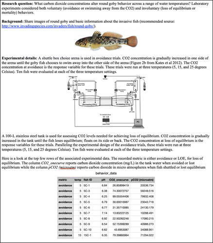
Cupp et al. (2017a) experimentally tracked carbon dioxide exposure concentrations needed to achieve avoidance or loss of equilibrium orientation (the fish equivalent of human balance) in the invasive round goby fish at three different temperatures (5, 10, and 15${}^{°}$ C). We used the resulting data (Cupp et al. 2017b) because we could readily explain the data’s structure and the well-designed experiment could easily be explained to non-biology majors. We gave students the dataset (Cupp et al. 2017b) and research questions from Cupp et al. (2017a). We shared pictures of the types of tanks used in the avoidance and loss of equilibrium trials and pictures of round goby fish to help build the contextual story for the project (Figure 2). The students were tasked with conducting an appropriate analysis and writing a statistical methods and results section for a research manuscript (Textbox 2).

Fig. 2 Example details for introducing the round goby fish task to students.

Textbox 2: Student assessment 1 for round goby data.

Based on the provided dataset and the associated research question, select and carry out an appropriate statistical analysis. Based on this work, write the statistical methods and results sections of a research paper intended for publication in a biology or ecology journal.

Methods section:

• Should note all statistical procedures used in just enough detail that another researcher could reproduce the work. Avoid too much detail (do not state ${\mathrm{H}}_0$, do not note exact code syntax, etc.)

• Note software used, name and version number.

• Note the significance level used for hypothesis tests.

• Do not include any results or conclusions in the methods section.

Results section:

• Include relevant summary statistics for the dataset (in text, table, and/or graphic form). Use your judgment to decide how the data can best be presented in a complete, yet digestible way.

• Report results of the statistical procedures noted in the methods section. State conclusions in sentence form with supporting statistical details noted in parentheses. For example: There is significant evidence that mean study time of college students somehow differs by class years (ANOVA, ${\mathrm{F}}_{3,155}=42.1,p<0.0001$). In particular, first year students study significantly more hours on average than seniors (Tukey’s HSD, p = 0.021).

The round goby dataset required decision-making for students. The students needed to think about the research question of interest in deciding strategy for analysis rather than leaning exclusively on data structure. For example, what features are in the dataset that are not narrated in the research question and explanation of the experimental design? Additionally, there was an imbalance in sample size between treatment groups with either 9 or 10 fish observed per treatment. Students had to consider the impacts of this imbalance. Students also had to think about analyzing subsections of the data or the entire dataset. Specifically, are avoidance and loss of equilibrium two separate experiments? Or can they be reasonably pooled into a single analysis? Lastly, students had to create descriptive statistics, plots, and models of potential value. Students had to think about how to communicate a complete story. For example, does a single, well-designed plot or table capture their story, or do they need multiple plots and tables? Likewise, when is it better to report a test statistic and p-value versus an estimated effect size?

For the round goby example, Cupp et al. (2017a) includes succinct statistical methods and results sections for students to benchmark their final solutions against as an “answer key” for the project. We had students think about why the F-statistics may not match exactly even if the same statistical method was applied by both the students and original authors. For this example, we specifically talked about types of sums of squares (e.g., sum of squares from sequential fitting of terms vs. fitting each term last) and how they differ when sample sizes are not perfectly balanced.

This project could be addressed using a pair of one-way ANOVA models (one for avoidance and one for LOE) or using a single two-way ANOVA model. Both methodologies are reasonable choices in this situation. The temperature setting of experimental runs (5, 15, or 25 degrees C) could be treated as either a numeric predictor variable or as a factor. There are strengths/weaknesses to each of these options. In this context, treating temperature as a factor is the better choice as the pattern in CO2 is not linear across temperatures. However, when treating temperature as a factor, we are not able to interpolate estimated CO2 values for temperatures between 5, 15, and 25 degrees C as we would be able to do if temperature were treated as a linear term.

4.2 Sea Lamprey

Schloesser et al. (2018) examined the use of environmental DNA (eDNA) for detecting the presence and possibly estimating the density of invasive sea lamprey. The lab-based experiment had a nested structure with multiple tanks holding one of four different sea lamprey densities: 0, 2, 20, and 200 sea lamprey per tank. Multiple samples were taken from each tank, with individual samples being sub-sampled multiple times using quantitative polymerase chain reaction (qPCR). The response variable was the number of copies of eDNA detected using qPCR. The resulting data (Schloesser 2017) contained a moderately complex structure. Students were required to make decisions about the data and the analysis. The overview of this assessment is shown in Figure 3. The related assignment given to students was similar to Textbox 2.

Fig. 3 Example details for introducing the sea lamprey task to students.

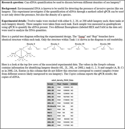
First, students had to think about how to parse the data. The identifying information on density, tank, and sample were concatenated in a single field in the raw data file (e.g., “200L-2A” for a stocking density of 200 lampreys in tank 2, sample A). Most nested statistical models require breaking this information into separate fields. Second, what statistical model correctly reflected the nested structure that was apparent in the experimental design? Third, was it acceptable to average across qPCR replicates? What is gained/lost in doing so? Fourth, how were missing values handled? Was there a difference in how missing response values and those noted as too few to count are handled? Fifth, how were various control tanks used in the analysis (well-water control, 0 sea lamprey as control, etc.)?

This project proved to be a prime example of the value in providing students with authentic data, with quirks and caveats that are not typically reflected in clean textbook exercises. In working with this dataset, no students caught the need to parse the concatenated fields in the first round of project drafts. Even when there was a sense of nesting in the description of the experimental design (with replicates nested in samples nested in tanks), the students simply fit a one-factor model and made a one-dimensional plot with the concatenated tank/sample/rep field as the only predictor variable. This was a naturally occurring data feature that students had not previously encountered and had no training in how to recognize or address. The first round of peer and instructor feedback proved essential in moving everyone toward a quality final product. The wrestling with and looking at the data from multiple angles created a sense of frustration and left the students feeling that things were not quite right. Based upon anecdotal conversations with students and alumni from our program, this feeling left a stronger and more long-lasting impression on the student’s learning than a simple note at the outset on data cleaning steps to mindlessly follow. This learning opportunity also helps the students to see an important lesson for applied statistics: “The only method to obtain experience is through experience.” That is to say, working with real problems will provide more learning opportunities, than nice textbook problems. We also have found, that as statistical practitioners, we often have learned the most when we fail and learn how to recover from initial failures. We hope examples like these help our students see how to not only gracefully fail, but also recover from setbacks and failure.

4.3 Infected Grasses Article Reproduction

Borer et al. (2010) examined the dynamics between grasses and vector-borne viruses. They released their data as supplemental material to their paper. In this case, students were given the published article (Borer et al. 2010) and associated tables/appendices at the outset. The student’s assignment was to recreate portions of the analysis from the article and produce an associated critique. This type of statistics is sometimes called “forensic statistics,” something done routinely by some medical institutes before repeating trials from other institutions and discussed by statisticians in commentaries such Baggerly and Berry (2011).

For this assignment, students received a peer-reviewed published article related to the project dataset with the initial project assignment (Textbox 3). They were tasked with recreating the primary statistical model reported in the results section of the article along with one plot and two tables from the article. The data structure for this project was notably more complex than in other assignments in the course. The students came up with many questions as they attempted to recreate the work and results. Several of these questions did not have clear answers.

This assignment gave students experience with more sophisticated data manipulation and highlighted the importance of clear and complete narration of methods. Students were not able to fully reproduce the article (nor was the instructor) based on the information provided within it. Their work attempting to recreate the results of the article informed their critique of it. The students were able to call out strengths and weaknesses in the statistical decisions and the communication of these decisions. A noteworthy observation about this dataset was that the authors published the data only within the article and supplemental materials. They did not release it as a formal data product such as a USGS data release (Faundeen et al. 2014; Faundeen and Hutchison 2017) or Zendodo (Peters et al. 2017) that require metadata, which would have assisted in recreating their results.

Textbox 3: Student assessment for forensic statistics project recreating infected grass paper.

Based on the provided research paper and associated data:

1. Reproduce the infection model fit and results (Table S4, Table S5, Figure 2b) along with related descriptive statistics. All data cleaning and wrangling should be done using R. Your reproduction work should be in a single R Markdown file that includes both R code and clarifying narration of your process. Submit both the.rmd file and the knit document.

2. Critique the research paper’s writing of statistical methods and results. Your comments should note both strengths and weaknesses. Was the paper’s described methodology adequate to guide your reproduction of their work?

3. Create a general list of guiding principles for statistical writing based off your own writing on earlier projects and your recreation/critique of this article.

Supplementary Materials

See https://github.com/bbennie/Goby for additional online supplementary materials. This repository includes example R code for the first project described in the article (round goby).

Acknowledgments

We thank H.M. Thompson for reading through an earlier version of this manuscript.

Disclosure Statement

The authors report there are no competing interests to declare.

Data Availability Statement

Example datasets have been previously published as standalone data releases (i.e., Cupp et al. 2017b; Schloesser 2017; Borer et al. 2016).

Additional information

Funding

RAE was supported by funding from the USGS Ecosystem Mission Area’s Biological Threats and Invasive Species Program.

Appendix A:

Scoring rubric used by instructor for final paper submission for student datasets analyses projects

Table

Context
8	7	6	5	4	3	2	1	0
		Writing aligns with the assigned audience, author’s voice shows credibility, assigned genre is used						Writing misaligns with the assigned audience, author’s voice lacks credibility, assigned genre is not used
Structure
10	9	8	6	5	4	2	1	0
		Writing is well-organized with methods and results cleanly segregated and sections labeled appropriately. Text, numeric summaries, and graphs complement one another well and are clearly labeled when appropriate.
Knowledge
16	14	12	10	8	6	4	2	0
		Statistical methods are selected and applied correctly. Method choices are justified/defended when appropriate. Statistical vocabulary is used correctly.
Focus
10	9	8	6	5	4	2	1	0
		Directly addresses the primary research question with a complete response. Added-value for concisely providing summary information on all available variables, even those peripheral to the core research question.
Design
8	7	6	5	4	3	2	1	0
		Effective use of tables/figures/summary statistics to communicate key features of data and analytic results. Telling a complete story in an audience-friendly way.
Conventions
8	7	6	5	4	3	2	1	0
		Correct grammar and spelling, citation of software is included, significance level is clearly stated.

Appendix B:

Prompts for Student Peer-Reviews of Statistical Projects

Paper authored by:

Paper reviewed by:

Note at least one strength of the draft

Make at least two suggestions for improving the draft

References

- American Statistical Association. (2014), Curriculum Guidelines for Undergraduate Programs in Statistical Science, Alexandria, VA: American Statistical Association.
- Baggerly, K. A., and Berry, D. A. (2011), “Reproducible Research,” AMSTAT News: The Membership Magazine of the American Statistical Association, American Statistical Association, pp. 16–17.
- Borer, E. T., Seabloom, E. W., Mitchell, C. E., and Power, A. G. (2010), “Local Context Drives Infection of Grasses by Vector-borne Generalist Viruses: Local vs. Regional Context and Infection rRisk,” Ecology Letters, 13, 810–818. DOI: 10.1111/j.1461-0248.2010.01475.x.
- Borer, E. T., Seabloom, E. W., Mitchell, C. E., and Power, A. G. (2016), “Data From: Local Context Drives Infection of Grasses by Vector-borne Generalist Viruses,” Dryad, Dataset, DOI: 10.5061/dryad.22dt8.
- Bozeman, B., and Boardman, C. (2009), “Broad Impacts and Narrow Perspectives: Passing the Buck on Science and Social Impacts,” Social Epistemology, 23, 183–198. DOI: 10.1080/02691720903364019.
- Cupp, A., Tix, J., Smerud, J., Erickson, R., Fredricks, K., Amberg, J., Suski, C., and Wakeman, R. (2017a), “Using Dissolved Carbon Dioxide to Alter the Behavior of Invasive Round Goby,” Management of Biological Invasions, 8, 567–574. DOI: 10.3391/mbi.2017.8.4.12.
- Cupp, A., Tix, J., Smerud, J., Erickson, R., Fredricks, K., Amberg, J., Suski, C., and Wakeman, R. (2017b), Using Dissolved Carbon Dioxide to Alter the Behavior of Invasive Round Goby, Reston, VA: U.S. Geological Survey Data Release. DOI: 10.5066/F7BZ650Q.
- Deming, W. E. (1972), “Code of Professional Conduct: A Personal View,” International Statistical Review/Revue Internationale de Statistique, 40, 215. DOI: 10.2307/1402763.
- Engel, J. (2017), “Statistical Literacy For Active Citizenship: A Call for Data Science Education,” Statistics Education Research Journal, 16, 44–49. DOI: 10.52041/serj.v16i1.213.
- Erickson, R. A., Burnett, J. L., Wiltermuth, M. T., Bulliner, E. A., and Hsu, L. (2021), “Paths to Computational Fluency for Natural Resource Educators, Researchers, and Managers,” Natural Resource Modeling, 34, e12318. DOI: 10.1111/nrm.12318.
- Faundeen, J., Burley, T. E., Carlino, J. A., Govoni, D. L., Henkel, H. S., Holl, S. L., Hutchison, V. B., Martín, E., Montgomery, E. T., Ladino, C., Tessler, S., and Zolly, L. S. (2014), “The United States Geological Survey Science Data Lifecycle Model,” Open-File Report, Report, Reston, VA, p. 12. DOI: 10.3133/ofr20131265.
- Faundeen, J., and Hutchison, V. (2017), “The Evolution, Approval and Implementation of the U.S. Geological Survey Science Data Lifecycle Model,” Journal of eScience Librarianship, 6, e1117. DOI: 10.7191/jeslib.2017.1117.
- Kates, D., Dennis, C., Noatch, M. R., and Suski, C. D. (2012), “Response of Native and Invasive Fishes to Carbon Dioxide: Potential for a Nonphysical Barrier to Fish Dispersal,” Canadian Journal of Fisheries and Aquatic Sciences, 69, 1748–1759. DOI: 10.1139/f2012-102.
- Kenett, R., and Thyregod, P. (2006), “Aspects of Statistical Consulting not Taught by Academia,” Statistica Neerlandica, 60, 396–411. DOI: 10.1111/j.1467-9574.2006.00327.x.
- Lanie, A. D., Jayaratne, T. E., Sheldon, J. P., Kardia, S. L. R., Anderson, E. S., Feldbaum, M., & Petty, E. M. (2004), “Exploring the Public Understanding of Basic Genetic Concepts,” Journal of Genetic Counseling, 13, 305–320. DOI: 10.1023/B:JOGC.0000035524.66944.6d.
- Malin, B. A., Emam, K. E., and O’Keefe, C. M. (2013), “Biomedical Data Privacy: Problems, Perspectives, and Recent Advances,” Journal of the American Medical Informatics Association, 20, 2–6. DOI: 10.1136/amiajnl-2012-001509.
- Mishra, P., Pandey, C., Singh, U., Keshri, A., and Sabaretnam, M. (2019), “Selection of Appropriate Statistical Methods for Data Analysis,” Annals of Cardiac Anaesthesia, 22, 297–301. DOI: 10.4103/aca.ACA_248_18.
- OPEN Data Act. (2007), OPEN Data Act, U.S. Code.
- Peters, I., Kraker, P., Lex, E., Gumpenberger, C., and Gorraiz, J. I. (2017), “Zenodo in the Spotlight of Traditional and New Metrics,” Frontiers in Research Metrics and Analytics, 2, 13. DOI: 10.3389/frma.2017.00013.
- Schloesser, N. (2017), Sea Lamprey Quantitative Environmental DNA Surveillance: Data, Reston, VA: U.S. Geological Survey Data Release. DOI: 10.5066/F7DR2TD0.
- Schloesser, N., Merkes, C. M., Rees, C., Amberg, J. J., Steeves, T., and Docker, M. (2018), “Correlating Sea Lamprey Density with Environmental DNA Detections in the Lab,” Management of Biological Invasions, 9, 483–495. DOI: 10.3391/mbi.2018.9.4.11.
- Wickham, H. (2014), “Tidy Data,” Journal of Statistical Software, 59, 1–23. DOI: 10.18637/jss.v059.i10.