Active-Learning Class Activities and Shiny Applications for Teaching Support Vector Classifiers

Abstract

Support vector classifiers are one of the most popular linear classification techniques for binary classification. Different from some commonly seen model fitting criteria in statistics, such as the ordinary least squares criterion and the maximum likelihood method, its algorithm depends on an optimization problem under constraints, which is unconventional to many students in a second or third course in statistics or data science. As a result, this topic is often not as intuitive to students as some of the more traditional statistical modeling tools. In order to facilitate students’ mastery of the topic and promote active learning, we developed some in-class activities and their accompanying Shiny applications for teaching support vector classifiers. The designed course materials aim at engaging students through group work and solidifying students’ understanding of the algorithm via hands-on explorations. The Shiny applications offer interactive demonstration of the changes of the components of a support vector classifier when altering its determining parameters. With the goal of benefiting the broader statistics and data science education community, we have made the developed Shiny applications publicly available. In addition, a detailed in-class activity worksheet and a real data example are also provided in the online supplementary materials.

KEYWORDS:

• Binary classification
• Hands-on learning
• Machine learning
• Multivariate data analysis
• Teamwork

1 Introduction

Over the past couple of decades, large and complex datasets have become easily stored and publicly available. Consequently, there has been a general trend toward using data in decision making. In the era of big data, it is vital for statistics and data science educators to equip our students with advanced modeling skills so that they are capable of turning these data into useful information. Therefore, teaching statistical modeling techniques with an emphasis on multivariate thinking has become an essential part of undergraduate statistics and data science education. In the American Statistical Association report on Curriculum Guidelines for Undergraduate Programs in Statistical Science (Horton et al. 2014), statistical modeling, including multivariate data analysis, has been identified as one of the core topics for the undergraduate statistics and data science curriculum.

One of the most important practical problems in statistics and data science is classification, where one is interested in building a statistical model, or developing a fitting algorithm, that correctly categorizes observations into different classes. There have been a number of different approaches developed so far for the task of classification, such as regression-based methods (e.g., logistic or probit regression, see Kutner, Nachtsheim, and Neter 2005) and Bayesian-based techniques (e.g., naive Bayes classifier and multivariate discriminant analysis, see James et al. 2013). Among them, support vector classifiers and support vector machines stand out as powerful practical tools which are often among the topics in a second or third course in statistics or data science, including Multivariate Data Analysis, Data Mining, Statistical Learning, and Machine Learning (Berk 2008; Izenman 2008; Hastie et al. 2009; James et al. 2013). However, support vector classifiers and support vector machines are formulated as an optimization problem under constraints. As a result, they are not as intuitive or accessible to students as some of the more traditional statistical models, such as linear regression or generalized linear regression. Consequently, teaching these methods via a pure lecture-style lesson often does not yield satisfactory learning outcomes. Active learning practice has been emphasized in undergraduate statistics education in recent decade (Armbruster et al. 2009; Freeman et al. 2014; Misseyanni et al. 2018). Many statistics educators have employed active learning into classroom teaching and received positive results (Carlson and Winquist 2011; Loux, Varner, and VanNatta 2016; Adair, Jaeger, and Price 2018; Lesser et al. 2019; Eadie et al. 2019). As statistics educators, one of our primary goals is to effectively help our students master the knowledge and skills taught in our classes. Over the past years, both of us (the authors) have engaged in developing educational tools and hands-on learning activities for teaching statistics at the undergraduate level. Through our informal assessments of integrating active learning components into our classrooms, we found that our students were uniformly positive about those activities. What is more, they seemed to have a better understanding on the related topics, as reflected during the in-class discussions as well as in the subsequent tests. In addition to involving active learning in introductory-level statistics courses, we also found that incorporating hands-on group activities and interactive demonstrations greatly facilitates students’ mastery of some more challenging concepts. Our finding also coincides with the current practice of employing active learning, that is, “learning by doing,” into statistics education in recent decades (Garfield 1993; Gnanadesikan et al. 1997; Schwartz 2013; Eadie et al. 2019). From the pedagogical research perspective, active learning has been shown to be effective in enhancing the recall of short-term and long-term information (Prince 2004; Misseyanni et al. 2018), fostering critical thinking, facilitating classroom interaction and collaboration, and engaging students to better master the knowledge. Many statistics and data science educators have contributed to this practice by sharing their innovative teaching tools (Cai and Wang 2020; Di Iorio and Vantini 2021; Wang et al. 2021), thought-provoking case studies (Wagaman 2016; Peng et al. 2021; Peterson and Ziegler 2021), and inspiring teaching experiences through various channels. We hope that our paper can serve as a valuable addition to further the effort of promoting active learning in the classroom.

The Guidelines for Assessment and Instruction in Statistics Education (GAISE College Report) (Carver et al. 2016), one of the resources statistics educators often refer to, advocates the introduction of multivariate thinking and hands-on teaching activities in undergraduate statistics education. Following their calls, we developed a number of active-learning in-class activities and some Shiny applications (Chang et al. 2022) that can be used for teaching the topic of support vector classifiers. The developed teaching materials and lesson plan aim at improving students’ understanding of the topic and promoting interactive learning environment. In addition, we hope that by sharing our work with the greater statistics and data science community, they can potentially benefit a broader audience of students beyond our own campuses.

The rest of the article is organized as follows: in Section 2 we outline basic concepts and give a general introduction of the topic on support vector classifiers. We then explain our developed teaching materials, including active-learning activities and Shiny applications, in Section 3. We conclude our article with some discussions in Section 4. An activity worksheet, its solution, and a real data example on handwriting recognition are included in the supplementary materials.

2 Background and Motivation

Binary classification is one of the most practical problems in statistics and machine learning. The goal is to correctly classify instances into two classes based on a set of attributes. It belongs to supervised learning, where the training dataset contains a variable (i.e., the response of interest) that records the true (binary) labels of the observations, and there are instances from each class (i.e., label) in the training dataset. This is in contrast to unsupervised learning, such as clustering for instance, where one aims to partition observations in a given dataset into groups based on a set of attributes without any knowledge of the true labels so that instances clustered within the same group share more in common. There are many available statistical tools for the task of binary classification, as discussed in Section 1. Among them, support vector classifiers stand out as popular techniques in statistics and machine learning.

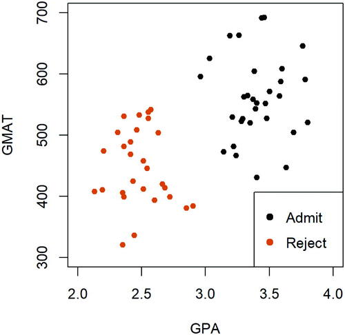
The first formal appearance of this technique can be found in Vapnik (1995) and Vapnik and Cortes (1995). It was originally motivated by a binary classification problem, where one aims to find an optimal hyperplane in ${\mathbf{R}}^k(k\ge 2)$ that correctly classifies observations into two categories. Figure 2.1 presents a simple example based on an admission dataset that contains observations of test scores on GPA (X₁) and GMAT (X₂) of n = 59 applicants from the admission office of a business school’s graduate programs (Johnson and Wichern 2014) (In this visualization, we trimmed the data by removing 5 borderline observations so that the two classes can be linearly separated. Discussion using the full dataset will be presented later). The response of interest, Y, is the admission decision, labeled as either “admit” (i.e., 1) or “reject” (i.e.,–1). From the plot, it is easy to see that the given feature space is linearly separable. That is, one can find a straight line that perfectly separates the two classes of applicants. Finding the best linear decision boundary is the goal of support vector classifiers. More discussion on support vector classifiers, including notations and formal definitions, will follow in the sections below.

Fig. 2.1 Display of an admission dataset (trimmed) for the task of binary classification.

The topic of support vector classifiers is often taught before the introduction of support vector machines. The latter tool is more technically demanding, as it first requires instructors to explain the kernel solution of a support vector classifier with the help of a linear kernel, and then extend the solution to employing a nonlinear kernel function in order to attain a nonlinear decision boundary in the feature space. In this article, we only focus on the discussion of teaching support vector classifiers, which is often covered within one 60 to 75-min class meeting.

2.1 Notations and Definitions

We first state some general definitions and technical notations, which are connected to the learning goals stated later. Consider a training sample of size n with k (quantitative) predictors, denoted as ${\mathbf{X}}_1,\dots ,{\mathbf{X}}_n$, where ${\mathbf{X}}_i=(X_{i,1},\dots ,X_{i,k})\text{ for }1\le i\le n$, and a binary categorical response Y. Our primary goal here is to identify a linear classifier, defined by a hyperplane in ${\mathbf{R}}^k$, that separates the two classes of observation as accurately as possible. Before diving into the technical details of support vector classifiers, we start with a simple scenario where the feature space is linearly separable in the sense that there exists a separating hyperplane in ${\mathbf{R}}^k$ that can perfectly classify observations in the training dataset into two groups.

Recall that a hyperplane in ${\mathbf{R}}^k$ can be generally written as (1) $${\beta }_0+{\beta }_1{X}_1+\cdots +{\beta }_k{X}_k=0.$$(1)

Mathematically speaking, the expression of a hyperplane is not unique, unless one imposes certain constraint on its coefficients. For instance, one can simply multiply a nonzero constant on both sides of the equation, for example, $a({\beta }_0+{\beta }_1{X}_1+\cdots +{\beta }_k{X}_k)=0(a\ne 0)$, and arrive at the same hyperplane. In the trivial case where the dimension of the feature space is k = 1 (i.e., a 1D feature space), a hyperplane is a single point; in a 2D space, a hyperplane is a straight line; in a 3D space, a hyperplane is simply a plane. For instance, a separating hyperplane for the admission dataset in Figure 2.1 can be written as ${\beta }_0+{\beta }_1{X}_1+{\beta }_2{X}_2=0$, where $X_1=\text{GPA}$ and $X_2=\text{GMAT}$.

In general, a hyperplane represents a linear decision boundary (i.e., a linear classifier) in the corresponding feature space. It separates the target feature space into two complementary half spaces. More specifically, observations falling to one side of the hyperplane would have their observed features satisfy ${\beta }_0+{\beta }_1{X}_1+\cdots +{\beta }_k{X}_k>0$, while data points lying on the other side correspond to ${\beta }_0+{\beta }_1{X}_1+\cdots +{\beta }_k{X}_k<0$. Hence, it is practically convenient to denote the labels of the binary categorical response as Y = 1 versus Y =–1.

Given an observation, say $({\mathbf{X}}_0,Y_0)$, its perpendicular distance to the hyperplane ${\beta }_0+{\beta }_1{X}_1+\cdots +{\beta }_k{X}_k=0$ can be written as $$d_0=\frac{Y_0({\beta }_0+{\beta }_1{X}_{0,1}+\cdots +{\beta }_k{X}_{0,k})}{\left|\right|\mathit{\beta }|{|}_2},$$where $\left|\right|\mathit{\beta }|{|}_2=\sqrt{{\sum }_{\mathcal{l}=1}^k{\beta }_{\mathcal{l}}^2}$ is the L₂ norm of $\mathit{\beta }=({\beta }_1,\dots ,{\beta }_k)$, that is, all coefficients except the intercept term. In addition, the smallest such distance in a (training) dataset is called the margin, denoted by M: $$M=\underset{{}_{i=1,\dots ,n}}{\min }{d}_i.$$

Given a separating hyperplane, any observation whose distance to the decision boundary is equal to the margin is referred to as a support vector.

2.2 Linearly Separable Case

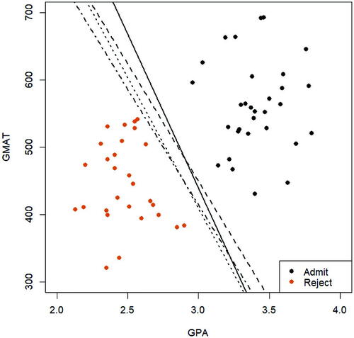
Recall the admission dataset displayed in Figure 2.1. As easily noted in the graph, this is a linearly separable feature space. In such a case, there are infinitely many separating hyperplanes that can perfectly separate the two classes of observations. Figure 2.2 displays a few such separating lines. In practice, there is a need to identify the best decision boundary under certain criterion. One possible approach is to find the separating hyperplane that yields the largest margin M, so that the two classes of observations are as “distant” as possible. A hyperplane that maximizes the margin is also more robust to data changes (James et al. 2013). As a result, such a classifier tends to produce accurate results on an independent dataset. This method is often referred to as the maximum margin classifier. Its formal definition is given below.

Fig. 2.2 Display of an admission dataset (trimmed) with a linearly separable feature space. A few possible separating lines are shown in the plot, all of which can perfectly classify the two groups of observations.

Definition 2.1.

Given a linearly separable feature space in ${\mathbf{R}}^k$ and a training sample of size n, the maximum margin classifier is a separating hyperplane that maximizes the margin. That is, the maximum margin classifier satisfies $$\begin{array}{c}({\beta }_0,{\beta }_1,\dots ,{\beta }_k)\\ =\arg \underset{{}_{{\beta }_0,\dots ,{\beta }_k}}{\max }\frac{1}{\left|\right|\mathit{\beta }|{|}_2}\underset{{}_{i=1,\dots ,n}}{\min }\left\{Y_i({\beta }_0+{\beta }_1{X}_{i,0}+\cdots +{\beta }_k{X}_{i,k})\right\}\end{array}$$

Since the expression of a hyperplane is not unique, one can rewrite the same hyperplane as $a({\beta }_0+{\beta }_1{X}_1+\cdots +{\beta }_k{X}_k)=0$ with $a=1/M$. By this trick of rescaling, the margin always equals to 1, and the solution of the maximum margin classifier is simplified to (2) $$({\beta }_0,{\beta }_1,\dots ,{\beta }_k)=\arg \underset{{}_{{\beta }_1,\dots ,{\beta }_k}}{\min }\frac{1}{2}\left|\right|\mathit{\beta }|{|}_2,$$(2) subject to $Y_i({\beta }_0+{\beta }_1{x}_{i,1}+\cdots +{\beta }_k{x}_{i,k})\ge 1$ for $i=1,\dots ,n$.

2.3 Nonlinearly Separable Case

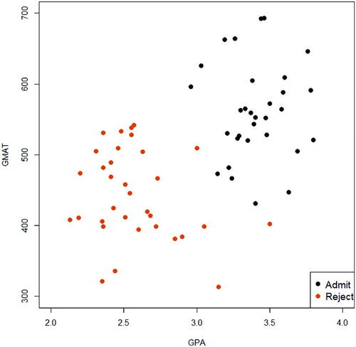
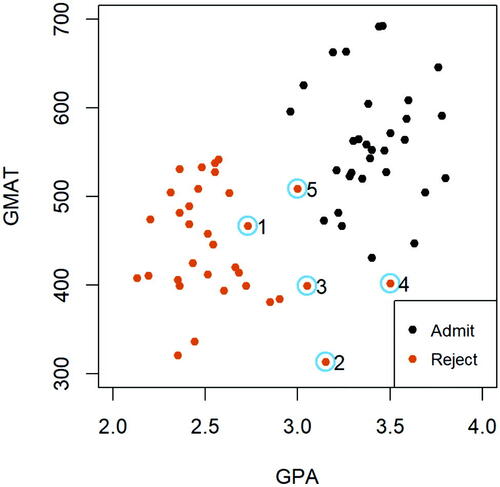
In practice, it is rarely the case that a feature space is perfectly separable by a linear decision boundary. Figure 2.3 displays the full admission dataset of size n = 64. Different from Figure 2.1, with the inclusion of five additional observations (all correspond to borderline decisions for admission that we later treated as rejections), it is clear that one can no longer identify a straight line that can perfectly separate the two classes of data points. In such cases, one has to allow some violations of the margin, which then might produce some misclassifications. This idea leads to the development of support vector classifiers, also referred to as the soft margin classifier.

Fig. 2.3 Display of the full admission dataset, where the feature space cannot be separated by a straight line.

Definition 2.2.

Given a feature space in ${\mathbf{R}}^k$ and a training sample of size n, a support vector classifier is a hyperplane, that is, ${\beta }_0+{\beta }_1{X}_1+\cdots +{\beta }_k{X}_k=0$ in ${\mathbf{R}}^k$, such that (3) $$({\beta }_0,\dots ,{\beta }_k)=\arg \underset{{}_{{\beta }_0,\dots ,{\beta }_k;{\zeta }_1,\dots ,{\zeta }_n}}{\min }\left\{\frac{1}{2}\left|\right|\mathit{\beta }|{|}_2+C_0\sum _{i=1}^n{\zeta }_i\right\},$$(3) subject to $$\begin{array}{c}{Y}_i({\beta }_0+{\beta }_1{x}_{i,1}+\cdots +{\beta }_k{x}_{i,k})\ge 1-{\zeta }_i,\\ {\zeta }_i\ge 0.\end{array}$$

The ζ_i’s parameters, also called “slack parameters” in linear programming, control whether each observation violates the margin. More specifically, if ${\zeta }_i=0$, the ith observation does not violate the margin and is correctly classified. However, when ${\zeta }_i>0$, the ith data point violates the margin, that is, its distance to the hyperplane is smaller than M which is rescaled to be 1. Furthermore, whenever ${\zeta }_i>1$, observation i is misclassified, lying on the incorrect side of the separating hyperplane.

The tuning parameter C₀ is often referred to as the “cost” parameter (see the “cost” argument in the svm() function in Section 3.6). When $C_0\to +\infty$, the overarching minimization problem in (3) would force all the slack parameters ζ_i’s to take a value of 0, and therefore the solution is reduced to the maximum margin classifier, provided that the feature space is linearly separable. On the contrary, as C₀ gets smaller, it is more likely for ζ_i’s to take positive values. As a result, there are more violations of the margin, possibly yielding a greater number of misclassified observations in the training dataset. The role of the “cost parameter” C₀ is further illustrated in our later discussion in Section 3 (see e.g., Figures 3.11–3.13) and is demonstrated in the Shiny apps we created as well.

On p. 382 of James et al. (2013) (edition 2), there is an alternative formulation for support vector classifiers. Given a dataset that is not rescaled (i.e., the margin is not rescaled to be 1), the algorithm can be described as an optimization problem under four constraints, namely, $$\underset{{}_{{\beta }_0,\dots ,{\beta }_k;{\zeta }_1,\dots ,{\zeta }_k;M}}{\max }M,$$subject to $$\begin{array}{c}\sum _{j=1}^k{\beta }_j=1,\\ Y_i({\beta }_0+{\beta }_1{x}_{i,1}+\cdots +{\beta }_k{x}_{i,k})\ge M(1-{\zeta }_i),\\ {\zeta }_i\ge 0,\\ \sum _{i=1}^k{\zeta }_i\le C.\end{array}$$

They call the tuning parameter C the “budget” which is related to the degree of violations of the margin. We chose to adopt the formulation stated in (3), since the “cost parameter” C₀ can be directly translated into the “cost” argument in the svm function in R. Our past experience also suggested that using the formulation in (3) made it easier for students to transition from mathematical formulation of the algorithm to real data implementation in R.

3 Developed Class Activities

We are teaching at two different private, four-year liberal arts colleges. We offer two courses that cover the topic of support vector classifiers: one is called Multivariate Data Analysis (textbooks used are Hastie et al. 2009 and Everitt and Hothorn 2011) and the other is Data Mining and Statistical Learning (the textbook is James et al. 2013). Both courses require students to have taken a second course in statistics (e.g., regression analysis or applied statistics) and have some mathematical background. More specifically, the first course (a 200-level course) requires students to have taken multivariable calculus, and the latter course (a 400-level course) includes both multivariable calculus and linear algebra as its mathematics prerequisites. These courses are counted as an elective toward the statistics major or minor, mathematics major or minor, and the data science major. Our class sizes are often small, capped at 20 or 25 students. However, the designed class activities and Shiny applications can be introduced to classes of moderate sizes, for example, 30–50 students. In addition, teaching the topic of support vector classifiers does not require advanced mathematics knowledge. For instance, understanding the algorithm of support vector classifiers does not require multivariable calculus or linear algebra. Hence, the developed course materials are accessible to a broader student audience with different mathematical preparations.

In the following developed class activities, we aim to accomplish the following learning goals:

1. Students will master the main concepts, such as hyperplane (linear classifier), margin, and support vector.

2. Students will thoroughly understand the mechanism of identifying a maximum margin classifier.

3. Given a support vector classifier fitted on a real dataset, students will be able to correctly identify the range for each of the parameter ζ_i’s (see Definition 2.2).

4. Students will understand the effects of the cost parameter C₀ in the algorithm of support vector classifiers given in (3).

5. Students will be able to fit a maximum margin classifier or a support vector classifier given a real data example, using the R function svm() in the e1071 package (Meyer et al. 2021).

3.1 Outline of the Lesson Plan

Prior to introducing the topic on support vector classifiers, students in our classes have been exposed to a few other techniques for binary classification, including regression-based methods (e.g., logistic regression and probit regression), linear and quadratic discriminant analysis, classification tree and ensemble methods. As a result, they are familiar with the difference between supervised leaning where the true labels are known and unsupervised learning, for example, clustering, where there are no observed labels for the observations.

The designed lesson is summarized as follows:

1. The lecture starts with a general introduction of the algorithm for support vector classifiers, as discussed in Section 2. Instructors may spend about 20 min on the motivation, background, and mathematical formulation of the algorithm.

2. Building upon a good understanding of the algorithm, the class is then divided into small groups, and every student will be distributed an activity worksheet (see the supplementary materials). They will be asked to complete the first activity in the worksheet in the case of a linearly separable feature space (see Sections 3.2 and 1 of the activity worksheet in the supplementary materials). The class may spend about 15 min on this activity.

3. Afterwards, attention is turned to a dataset that is not linearly separable. The formed small groups move on to work on the second in-class activity (see Sections 3.4 and 2 of the activity worksheet in the supplementary materials), which may take another 20 min of the class time. During the process of completing the activities, instructors may provide individual help and join the discussion of different groups.

4. In the end, the entire class shares their reflections and observations after these exercises, and the instructor may conclude the lesson by summarizing some key takeaways from the activities.

In what follows, we detail the two designed activities on maximum margin classifiers and support vector classifiers, along with demonstrations of the developed Shiny applications that accompany these hands-on exercises. A detailed activity worksheet and the data supporting the findings of this study can be found in the supplementary materials online.

3.2 Activity on Maximum Margin Classifiers

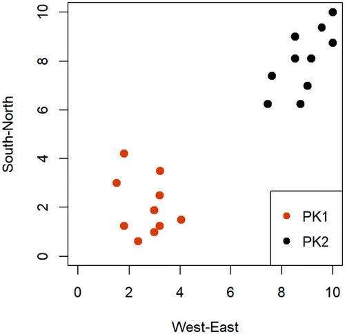
The first in-class group activity was designed with the objective of solidifying students’ understanding of basic concepts in maximum margin classifier, such as hyperplane, margin, and support vector. To engage students in active learning, we generated a dataset that represents a snapshot of static positions (i.e., X₁ and X₂ represent the geographic coordinates in a square field) of two classes of preschool children, each with 10 students, who are playing outside on a playground during recess. The response variable Y labels the class membership and is recorded as either “PK1” or “PK2”. Figure 3.1 displays the dataset, where the orange and black points indicate observations from each of the two classes. We acknowledge that this dataset is made up and not complex. There are a few motivations behind our choice of this “toy” dataset: first, since the two features in this dataset represent geographic coordinates in a square field, the distance between two students is the actual physical distance and therefore is very easy to understand. In addition, in the given context, we can motivate the proposal of a maximum margin classifier, that is, maximizing the margin, by relating to the the “social distancing” practice during the Covid-19 pandemic. We believe this connection facilitates students’ understanding of the algorithm. What is more, we want to ease students’ learning curve, so we choose to start with a simple example and help students thoroughly understand the concepts before moving to a more complex real dataset.

Fig. 3.1 Display of a preschool dataset where the feature space is linearly separable.

When presenting this dataset, instructors may raise some motivating questions as below:

• Given the static positions of the preschool children, do you think the two classes of students can be perfectly separated by a straight line (e.g., imagine stretching a long straight rope)?

• How can you express such a linear decision boundary in a two-dimensional space?

• How many such separating lines are there?

• What should we consider if we want to find the best separating line?

Next, we move on to consider a few such separating hyperplanes (i.e., straight lines in 2D), each being a candidate classifier that perfectly separates the two classes of observations. Figure 3.2 gives two examples.

Fig. 3.2 Two candidate separating lines (in blue) given the preschool dataset. Each line can perfectly separate the two classes of preschool students.

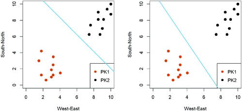
To better motivate the proposal of the maximum margin classifier, instructors may describe the margin as some sort of “social distancing” measure. Relating to the social distancing practice during the Covid-19 pandemic, it is then intuitive for one to seek a separating line that maximizes the social distance between the two classes of students. Referring back to the candidate separating lines in Figure 3.2, students are recommended to work in pairs or form small groups to answer the following questions:

1. In each plot, mark the length of the margin.

2. In each plot, circle all support vectors given the separating line.

   1. Do you think the given classifier in each panel is the maximum margin classifier? If not, how would you suggest to change the intercept and/or slope of the given separating line to achieve the maximum margin classifier?

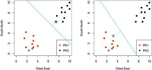
The answers to Questions #1 and #2 are presented in Figure 3.3. More information on the designed class activity and solution can be found in the supplementary materials.

Fig. 3.3 Display of the support vectors and margins given each of the separating lines for the preschool dataset (visualizations that addresses Questions 1 and 2).

Following Question #3, to further facilitate the discussion and enhance students’ understanding of the maximum margin classifier, we developed a Shiny application to illustrate the changes of the separating hyperplane, that is, a straight line in 2D, when altering its intercept and slope based on the PK dataset. We detail the functionalities of our developed Shiny application in the section below.

3.3 Shiny Application for Teaching Maximum Margin Classifiers

To facilitate students’ understanding of the basic concepts in maximum margin classifier, we developed the following Shiny application. The Shiny web applications can be found in this link. There are two selection tabs in the same web interface, namely, “Illustration of Maximum Margin Classifiers” and “Illustration of Support Vector Classifiers”. In this section we focus on introducing the first application (tab 1), and discussion of the second tab can be found in Section 3.5.

A screenshot of the first tab of Shiny application page is shown in Figure 3.4. This application displays the scatterplot of the PK dataset on the right side, overlaying a decision line with a given intercept and a slope, both of which can be selected by the users. For example, the screenshot in Figure 3.4 shows the decision line with an intercept of 8 and a slope of–0.8.

Fig. 3.4 A screenshot of the first Shiny application (tab 1). One the left-hand side, a user sets the intercept (8) and slope (–0.8) of a separating line, and the resulting decision line is displayed in the plot on the right-hand side.

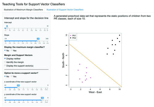
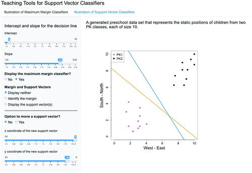
The left panel of the page provides user-friendly options to customize the display. More specifically, users may use the slider on the top of the panel to specify any values for the intercept and slope of the decision line, and the corresponding decision line will be automatically updated in the graph on the right. In addition, by selecting “Yes” for the question “Display the maximum margin classifier?”, the maximum margin classifier is also added to the scatterplot using a blue solid line, as shown in Figure 3.5.

Fig. 3.5 A comparison between a given decision line (orange) and the maximum margin classifier (blue). Given the separating line as specified in Figure 3.4, if one chooses to display the maximum margin classifier by responding “Yes” to the question on the left, the maximum margin classifier (in blue) is added to the plot.

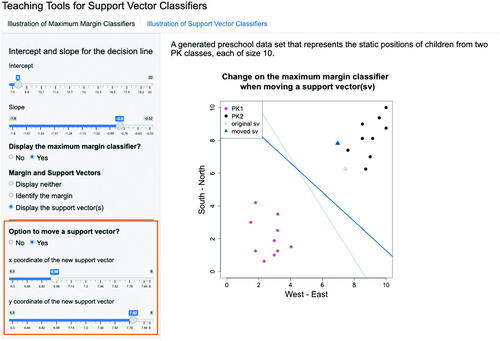
Additionally, users may also choose to compute and present the margin, and identify the support vector(s). Given a decision line with selected intercept and slope, users may check options under the selection menu “Margin and Support Vectors” to include other information in the visualization. For instance, when selecting “Identify the margin” option, the display will be updated to Figure 3.6, where the points from both categories that each is the closest to the decision line and their corresponding distances are shown. The application internally calculates the margin which is the smaller value between these two distances. In this example, the margin is shown to be 1.51. Furthermore, users may choose “Display the support vector(s)” to circle all support vectors in the plot, as shown in Figure 3.7. In both Figures 3.6 and 3.7 the selection for the question “Display the maximum margin classifier” is set to be “No”. When the selection is changed to “Yes,” the margin and support vectors for the maximum margin classifier are displayed, as seen in Figure 3.8. Finally, to illustrate the importance of support vectors in determining the maximum margin classifiers, there is an option to change the location of one support vector in the dataset. By selection “Option to move a support vector,” the user can change the x and y coordinates of one support vector. Then, the locations of both the original and new maximum margin classifiers are displayed in the plot, as shown in Figure 3.9. It is important to emphasize to students that in practice one cannot possibly move around any data point. This app feature only aims to demonstrate the dependency of a maximum margin classifier on its support vectors. In real life applications, one cannot alter any observations to achieve a different maximum margin classifier.

Fig. 3.6 Given the separating line as specified in Figure 3.4, if one checks the “Identify the margin” option from the selection menu on the left, the margin of the chosen separating line is calculated and presented on top of the graph window. Note that the option for “Display the maximum margin classifier?” is selected as “No”.

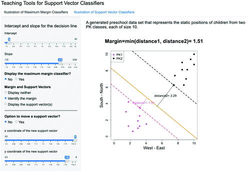
Fig. 3.7 Given the separating line as specified in Figure 3.4, if one chooses to “Display the support vector(s)”, the support vector is circled in the graph and the corresponding margin is calculated and presented. Note that the option for “Display the maximum margin classifier?” is selected as “No”.

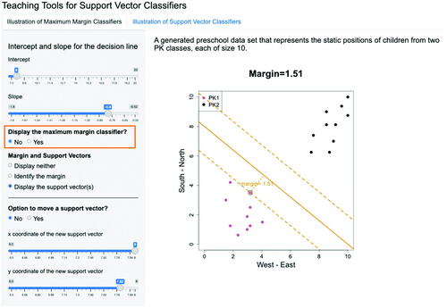
Fig. 3.8 Given the separating line as specified in Figure 3.4, after choosing “Display the maximum margin classifier”, the maximum margin classifier is displayed and the largest margin is calculated and presented in the graph. The difference between Figures 3.7 and 3.8 is whether the maximum margin classifier is displayed or not, as highlighted in the orange box.

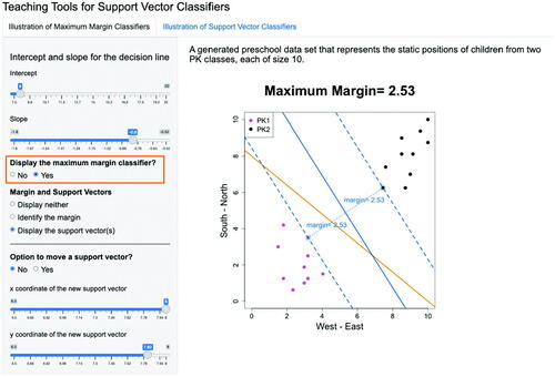
Fig. 3.9 Illustration of reliance of a maximum margin classifier on its support vectors. Here we choose to “Display the maximum margin classifier” and allows one to move one of the support vectors by checking the“Option to move a support vector”. Then, users can move the location of a support vector using the sliders to see how its position impacts the resulting maximum margin classifier. The original maximum margin classifier before moving the support vector is in light blue color and the new updated maximum margin classifier after moving the support vector is in darker blue color.

During a regular class session, instructors may incorporate the Shiny application into teaching by encouraging students to explore different combinations of the slope and the intercept of the decision line. The goal of this self-exploration is to guide them to discover a decision line that is as close to the maximum margin classifier as possible. Without revealing the true maximum margin classifier, the instructor can then direct the students to check the option “Identify the margin” and ask them to think whether the line they identified has the maximum margin in the updated graph. Given the same graph, the instructor may also ask the students to circle the support vectors and then compare their results to the answer by selecting “Display the support vector(s)”. Students can then display the maximum margin classifier by choosing “Yes” under the question “Display the maximum margin classifier?” and compare their decision line to the true maximum margin classifier. In the end, students may explore how the maximum margin classifier changes when altering the location of one support vector by selecting “Option to move a support vector” by using the sliders to determine the x and y coordinates of the new support vector.

3.4 Activity on Support Vector Classifiers

Next, we discuss active-learning in-class exercises for teaching support vector classifiers. In practice, we often need to deal with a classification dataset that cannot be perfectly separated by a linear decision boundary. For instance, Figures 3.10 displays the previously considered admission dataset after adding five extra points to the “Reject” group, circled and marked in the plot. As easily seen in the scatterplot, by including these five additional observations, there does not exist a straight line (i.e., a hyperplane in ${\mathbf{R}}^2$) that can perfectly distinguish observations between the two classes. Consequently, if we still wish to fit a linear classifier, we need to allow certain number of misclassifications.

Fig. 3.10 The full admission dataset. The difference between the full data and the trimmed data (Figure 2.1) is the inclusion of five observations, as circled in the graph.

Recall the optimization algorithm of a support vector classifier expressed in (3). As introduced earlier, the cost parameter C₀ controls the degree of violations of the margin. The three panels in Figure 3.11 present three different solutions of a support vector classifier, each based on a different value for the cost parameter C₀. After displaying these plots, the instructor may raise the following questions and encourage students to discuss them in small groups. In particular, we marked and labeled all support vectors in Figures 3.12 and 3.13 to ease the discussions within each student group.

Fig. 3.11 Display of support vector classifiers with three different cost parameters (i.e., 0.5, 1, and 10) based on the full admission dataset.

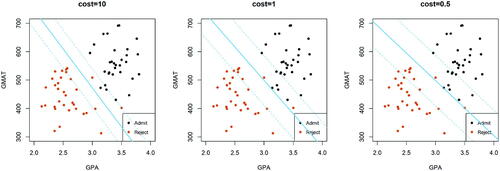
1. According to the Figure 3.11, what’s the effect of the cost parameter C₀ for a support vector classifier? Summarize your observations.

2. In Figures 3.12 and 3.13, the solid blue line represents the support vector classifier given the cost parameter value, and the dashed parallel lines have distance to the decision boundary equal to the margin. All support vectors in each plot are marked and labeled. Given a support vector, say observation i, can you point out the range of values for its corresponding tuning parameter ζ_i? That is, is ${\zeta }_i=0,0<{\zeta }_i<1$, or ${\zeta }_i>1$?

3. Following Question 2, what should be the value of ζ_i when point i is misclassified?

Fig. 3.12 Display of the support vector classifier using cost parameter $C_0=10$ based on the full admission dataset.

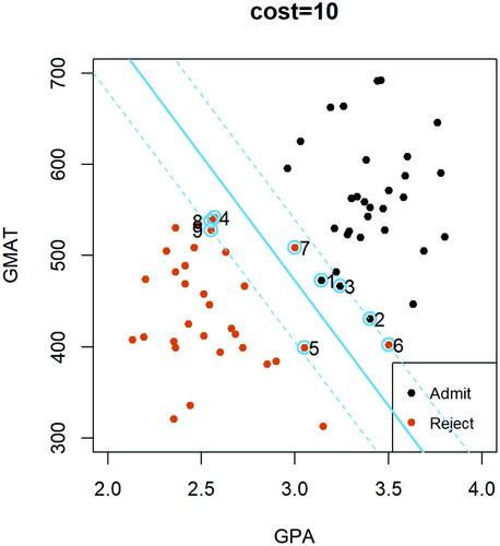
Fig. 3.13 Display of the support vector classifier with cost parameter $C_0=1$ based on the full admission dataset.

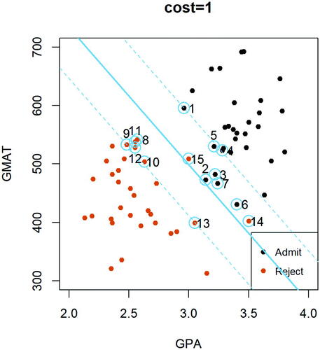
As can be seen in Figure 3.11, with a relatively small value for the cost parameter, for example, $C_0=0.5$, it is quite challenging to pin point all support vectors in the plot. Therefore, we created the following Shiny application based on the admission dataset that can be used during the small-group discussion in class when considering various values for the cost parameter C₀.

3.5 Shiny Application for Teaching Support Vector Classifiers

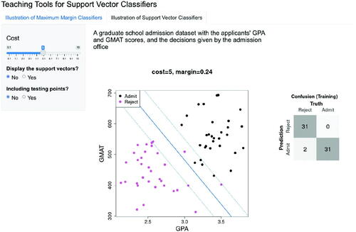
To enhance students’ understanding of support vector classifiers, we developed a second Shiny application which is accessible through a tab, called “Illustration of Support Vector Classifiers,” within the same interface of the app shown in Section 3.3. This app provides an interactive demonstration of the changes of the linear decision boundary, margin, margin lines, support vectors, number of violations of margin, and the number of misclassifications when altering the cost parameter of a support vector classifier. For example, in Figure 3.14, when setting the cost parameter to be 5 via the selection interval, the app shows the calculated margin (i.e., 0.24), as well as the margin lines which are displayed by the dashed blue lines on both sides of the support vector classifier.

Fig. 3.14 A screenshot of the second Shiny application based on the full admission dataset. Here we choose to set the cost parameter value to be 5, as specified using the sliding bar on the left, and not to display the support vectors. The resulting support vector classifier (solid blue line) and margin lines (dashed blue lines) are displayed in the graph. In addition, the confusion matrix is shown on the right.

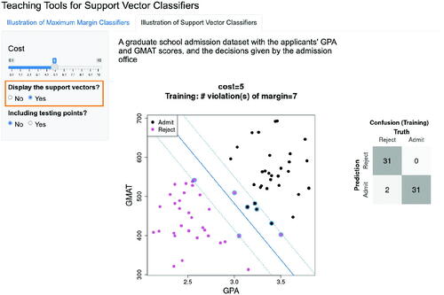
As an added feature, when selecting “Yes” for the question “Display the support vectors?”, all support vectors are circled within the same plot (see Figure 3.15). In addition, the corresponding confusion table for the classifier given the chosen cost parameter value is displayed on the right of the graph, and the number of observations that violate the margin are calculated and summarized on the top of the graph. Figure 3.15 shows that when the cost parameter equals 5, there are a total number of 7 observations that lie between the two margin lines, among which 2 are misclassified.

Fig. 3.15 Display of the same support vector classifier with cost parameter equal to 5, as shown in Figure 3.14. Here we choose to include the support vectors in the plot, by checking “Yes” for the question “Display support vectors?”. Consequently, all the support vectors are circled in the plot.

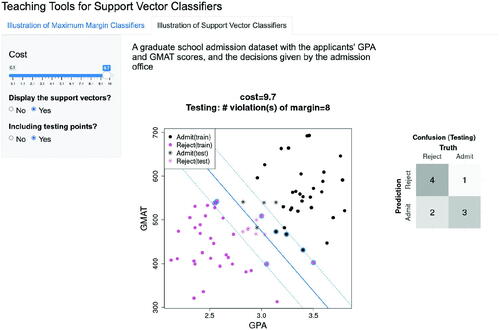
The app also has a functionality to evaluate the performance of a support vector classifier on a testing set with different values of the cost parameter. When selecting “Yes” for the question “Including testing points?”, 10 testing points are added to the plot (see Figure 3.16). The confusion table is then updated to present the results for the validation set. For instance, when the cost parameter equals 5, there are a total number of 9 testing observations that lie between the two margin lines, among which 2 are misclassified. As the cost parameter increases to 9.7 (see Figure 3.17), the number of misclassifications increases to 3. This observation reveals that the performance of a support vector classifier on an independent dataset does not necessarily improve as the cost parameter value increases.

Fig. 3.16 Display of the same support vector classifier with cost parameter equal to 5, as shown in Figure 3.14. Here we choose to include 5 test points, denoted by black or red asterisk in the plot. The classification results on the test points are reflected in the test confusing matrix on the right.

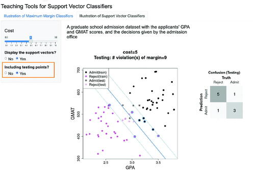
Fig. 3.17 Illustration of the effect of the cost parameter on classification performance in the test sample. Here we set the cost parameter to 9.7, instead of 5. The corresponding separating line (solid blue line) and margin lines (dashed blue lines) are updated in the graph. With a larger value of the cost parameter compared to Figure 3.16, although the number of violations of margin is down from 9 to 8, as shown on top of the graph, the test misclassification error increases as shown in the test confusion matrix.

3.6 R Implementations

By now, students should have a thorough understanding of the algorithms for the maximum margin classifiers and support vector classifiers. At the end of the lesson, if time permits, instructors may introduce the function(s) that can be used to fit such a linear classifier in R (or other statistical languages or software) (R Core Team 2022). (If the class time is already fully unitized after the in-class activities, the discussion on R implementations may be covered in a subsequent lesson.) In the following, we employ the R function svm() and illustrate its functionalities based on a real dataset that involves a higher-dimensional feature space. The function svm() is contained in the package e1071(Meyer et al. 2021) and is one of the available R functions that can be used to fit a support vector classifier or a support vector machine. We acknowledge that there are other available libraries and functions for employing support vector machines in R. For instance, the “kernlab” package (Karatzoglou, Smola, and Hornik 2022) can be considered for this purpose too. We chose e1071 due to the fact that this is a package that our students had used in the past and were familiar with. In addition, this package is also considered in the textbook we chose for our classes.

To get started, one first needs to require the e1071 package, and then can apply the function to fit a support vector classifier following the syntax shown below:

library(e1071)

svm(x, y, data, kernel="linear", cost)

Here, x represents a n × k data matrix of the observed features in the (training) dataset (k: the number of features; n: the sample size), y is a $n\times 1$ vector of labels, defined as a factor, and the “cost” argument specifies the cost parameter C₀ in (3). Given a linearly separable feature space, one may set C₀ to a sufficiently large number, and the function fits a maximum margin classifier. Given a feature space that is not linearly separable, one may tune the cost parameter by cross-validation using the function tune(). Since we focus on the discussion of support vector classifiers in this lesson, the kernel function is set to be linear. Extension to employing a nonlinear kernel to fit a support vector machine often cannot be discussed within the same class meeting, and therefore we omit the topic of support vector machines in this article.

To better demonstrate how to apply the svm() function to fit a support vector classifier in practice, we consider a real data example on handwriting recognition of digits 4 and 6. In our classes, we present this example using a computer and encourage our students to try things out using their individual computational notebooks at the same time. A detailed discussion of the real data example can be found in the supplementary materials online.

Support vector machines, with a nonlinear kernel function, are often discussed after introducing support vector classifiers. Although this paper only focuses on linear classification and support vector classifiers, we want to point out that the transition to the topic of support vector machines is through the kernel expression of the solution of support vector classifiers and by employing a nonlinear kernel function. The R implementation for support vector machines is similar as discussed in the article, except that the user needs to adjust the choice of the kernel function through the “kernel” argument in svm.

We acknowledge that there are other popular programming languages that can be used to fit support vector classifiers or support vector machines. For instance, in Python one may use the svm.SVC() function in the sklearn package to fit a support vector classifier.

4 Summary

This article introduces active-learning in-class activities and the accompanying Shiny applications for teaching support vector classifiers. The developed course materials aim at enhancing students’ understanding of the basic concepts and key components of the algorithm. The designed in-class activities can be completed through collaborative teamwork in small groups, which further promotes active learning and in-class participation. The developed course materials, including the activity worksheet, the real data example, and the accompanying Shiny applications, are all publicly available online. In a future project, we are interested in evaluating the efficacy and teaching outcomes of implementing the developed teaching materials.

As we are in the era of big data and fast-developing technologies, equipping our undergraduate students with advanced data analysis techniques becomes pressingly necessary and unquestionably crucial for their future successes. As undergraduate statistics and data science educators, we have been working hard to integrate more contemporary modeling tools into our classrooms. When teaching such advanced topics, such as support vector classifiers and support vector machines, to our eager students with background, it is important to make them accessible to and engage everyone. With that in mind, we echo the advocate of active learning, and hope that more statistics educators may join us in the undergraduate statistics community. Our developed learning tools serve as a little step to make modeling techniques, such as support vector classifiers, more accessible to a broader audience. And, we will continue our efforts in this direction and keep developing more open-resource teaching materials in the future.

Supplementary Materials

The online supplementary materials include a class activity worksheet, its solution, and a real data example on handwriting recognition.

Disclosure Statement

No potential conflict of interest was reported by the author(s).

Data Availability Statement

The datasets used in the activities and the R code used to create all figures in this article are openly available in Github https://github.com/xizhen-cai/ActiveLearning_SVM/.

References

- Adair, D., Jaeger, M., and Price, O. M. (2018), “Promoting Active Learning When Teaching Introductory Statistics and Probability Using a Portfolio Curriculum Approach,” International Journal of Higher Education, 7, 175–188. Available at https://eric.ed.gov/?id=EJ1175058. DOI: 10.5430/ijhe.v7n2p175.
- Armbruster, P., Patel, M., Johnson, E., and Weiss, M. (2009), “Active Learning and Student-Centered Pedagogy Improve Student Attitudes and Performance in Introductory Biology,” CBE–Life Sciences Education, 8, 203–213. DOI: 10.1187/cbe.09-03-0025.
- Berk, R. A. (2008), Statistical Learning from a Regression Perspective (Vol. 14), Cham: Springer.
- Cai, X., and Wang, Q. (2020), “Educational Tool and Hands-on Active-Learning Class Activity for Teaching Agglomerative Hierarchical Clustering,” Journal of Statistics Education, 28, 280–288. DOI: 10.1080/10691898.2020.1799727.
- Carlson, K. A., and Winquist, J. R. (2011), “Evaluating an Active Learning Approach to Teaching Introductory Statistics: A Classroom Workbook Approach,” Journal of Statistics Education, 19. DOI: 10.1080/10691898.2011.11889596.
- Carver, R., Everson, M., Gabrosek, J., Horton, N., Lock, R., Mocko, M., Rossman, A., Roswell, G. H., Velleman, P., Witmer, J., and Wood, B. (2016), Guidelines for Assessment and Instruction in Statistics Education (GAISE) College Report 2016,” The American Statistical Association. Available at https://www.amstat.org/docs/default-source/amstat-documents/gaisecollege_full.pdf.
- Chang, W., Cheng, J., Allaire, J. J., Sievert, C., Schloerke, B., Xie, Y., Allen, J., McPherson, J., Dipert, A., and Borges, B. (2022), shiny: Web Application Framework for R. R package version 1.7.4. Available at https://CRAN.R-project.org/package=shiny.
- Di Iorio, J., and Vantini, S. (2021), “How to Get Away with Statistics: Gamification of Multivariate Statistics,” Journal of Statistics and Data Science Education, 29, 241–250. DOI: 10.1080/26939169.2021.1997128.
- Eadie, G., Huppenkothen, D., Springford, A., and McCormick, T. (2019), “Introducing Bayesian Analysis With M&M’s: An Active-Learning Exercise for Undergraduates,” Journal of Statistics Education, 27, 60–67. DOI: 10.1080/10691898.2019.1604106.
- Everitt, B., and Hothorn, T. (2011), An Introduction to Applied Multivariate Analysis with R (1st ed.), New York: Springer.
- Freeman, S., Eddy, S. L., McDonough, M., Smith, M. K., Okoroafor, N., Jordt, H., and Wenderoth, M. P. (2014), “Active Learning Increases Student Performance in Science, Engineering, and Mathematics,” Proceedings of the National Academy of Sciences, 111, 8410–8415. DOI: 10.1073/pnas.1319030111.
- Garfield, J. (1993), “Teaching Statistics Using Small-Group Cooperative Learning,” Journal of Statistics Education, 1, 1–9. DOI: 10.1080/10691898.1993.11910455.
- Gnanadesikan, M., Scheaffer, R. L., Watkins, A. E., and Witmer, J. A. (1997), “An Activity-Based Statistics Course,” Journal of Statistics Education, 1, 1–16. DOI: 10.1007/978-1-4757-3843-8.
- Hastie, T., Tibshirani, R., Friedman, J. H., and Friedman, J. H. (2009), The Elements of Statistical Learning: Data Mining, Inference, and Prediction (Vol. 2), New York: Springer.
- Horton, N., Chance, B., Cohen, S., Grimshaw, S., Hardin, J., Hesterberg, T., Hoerl, R., Malone, C., Nichols, R., and Nolan, D. (2014), “Curriculum Guidelines for Undergraduate Programs in Statistical Science,” Available at https://www.amstat.org/asa/files/pdfs/EDU-guidelines2014-11-15.pdf.
- Izenman, A. (2008), Modern Multivariate Statistical Techniques. Regression, Classification and Manifold Learning, New York: Springer.
- James, G., Witten, D., Hastie, T., and Tibshirani, R. (2013), An Introduction to Statistical Learning, New York: Springer.
- Johnson, R. A., and Wichern, D. W. (2014), Applied Multivariate Statistical Analysis (Vol. 6), Noida: Pearson.
- Karatzoglou, A., Smola, A., and Hornik, K. (2022), kernlab: Kernel-Based Machine Learning Lab. R package version 0.9-31. Available at https://CRAN.R-project.org/package=kernlab
- Kutner, M. H., Nachtsheim, C. J., and Neter, J. (2005), Applied Linear Statistical Models (5th ed.), Boston: McGraw-Hill Irwin.
- Lesser, L. M., Pearl, D. K., Weber III, J. J., Dousa, D. M., Carey, R. P., and Haddad, S. A. (2019), “Developing Interactive Educational Songs for Introductory Statistics. Journal of Statistics Education, 27, 238–252. DOI: 10.1080/10691898.2019.1677533.
- Loux, T. M., Varner, S. E., and VanNatta, M. (2016), “Flipping an Introductory Biostatistics Course: A Case Study of Student Attitudes and Confidence,” Journal of Statistics Education, 24, 1–7. DOI: 10.1080/10691898.2016.1158017.
- Meyer, D., Dimitriadou, E., Hornik, K., Weingessel, A., and Leisch, F. (2021), e1071: Misc Functions of the Department of Statistics, Probability Theory Group (Formerly: E1071), TU Wien. R package version 1.7–9. Available at https://CRAN.R-project.org/package=e1071
- Misseyanni, A., Lytras, M., Papadopoulou, P., and Marouli, C. (2018), Active Learning Strategies in Higher Education: Teaching for Leadership, Innovation, and Creativity (1st ed.), Bingley: Emerald.
- Peng, R. D., Chen, A., Bridgeford, E., Leek, J. T., and Hicks, S. C. (2021), “Diagnosing Data Analytic Problems in the Classroom,” Journal of Statistics and Data Science Education, 29, 267–276. DOI: 10.1080/26939169.2021.1971586.
- Peterson, A. D., and Ziegler, L. (2021), “Building a Multiple Linear Regression Model with LEGO Brick Data,” Journal of Statistics and Data Science Education, 29, 297–303. DOI: 10.1080/26939169.2021.1946450.
- Prince, M. (2004), “Does Active Learning Work? A Review of the Research,” Journal of Engineering Education, 93, 223–231. DOI: 10.1002/j.2168-9830.2004.tb00809.x.
- R Core Team. (2022), R: A Language and Environment for Statistical Computing. Vienna, Austria: R Foundation for Statistical Computing. https://www.R-project.org/.
- Schwartz, T. A. (2013), “Teaching Principles of One-Way Analysis of Variance Using M&M’s Candy,” Journal of Statistics Education, 21, 1–13. DOI: 10.1080/10691898.2013.11889662.
- Vapnik, V. (1995). The Nature of Statistical Learning Theory, New York: Springer.
- Vapnik, V., and Cortes, C. (1995), “Support Vector Networks,” Machine Learning, 20, 273–297. DOI: 10.1007/BF00994018.
- Wagaman, A. (2016), “Meeting Student Needs for Multivariate Data Analysis: a Case Study in Teaching an Undergraduate Multivariate Data Analysis Course,” The American Statistician, 70, 405–412. DOI: 10.1080/00031305.2016.1201005.
- Wang, S. L., Zhang, A. Y., Messer, S., Wiesner, A., and Pearl, D. K. (2021), “Student-Developed Shiny Applications for Teaching Statistics,” Journal of Statistics and Data Science Education, 29, 218–227. DOI: 10.1080/26939169.2021.1995545.