A Geant4-based Monte Carlo study of a benchtop multi-pinhole X-ray fluorescence computed tomography imaging

Abstract

Background

X-ray fluorescence (XRF) computed tomography (XFCT) has shown promise for molecular imaging of metal nanoparticles such as gold nanoparticles (GNPs) and benchtop XFCT is under active development due to its easy access, low-cost instrumentation and operation.

Purpose

To validate the performance of a Geant4-based Monte Carlo (MC) model of a benchtop multi-pinhole XFCT system for quantitative imaging of GNPs.

Methods

The MC mode consisted of a fan-beam x-ray source (125 kVp), which was used to stimulate the emission of XRF from the GNPs, a phantom (3 cm in diameter) which included six or nine inserts (3 mm in diameter), each of which contained the same (1 wt. %) or various (0.08–1 wt. %) concentrations of GNPs, a multi-pinhole collimator which could acquire multiple projections simultaneously and a one-sided or two-sided two-dimensional (2D) detector. Various pinhole diameters (3.7, 2, 1, 0.5 and 0.25 mm) and various particle numbers (20, 40, 80 and 100 billion) were simulated and the results for single pinhole and multi-pinhole (9 pinholes) imaging were compared.

Results

The image resolution for a 1 mm multi-pinhole was between 0.88 and 1.38 mm. The detection limit for multi-pinhole operation was about 0.09 wt. %, while that for the single pinhole was about 0.13 wt. %. For a fixed number of pinholes, noise increased with decreasing number of photons.

Conclusion

The MC mode could acquire 2D slice images of the object without rotation and demonstrated that a multi-pinhole XFCT imaging system could be a potential bioimaging modality for nanomedical applications.

Keywords:

• Geant4
• Monte Carlo simulation
• multi-pinhole
• X-ray fluorescence computed tomography
• gold nanoparticles
• bioimaging modality

Introduction

X-ray fluorescence (XRF) analysis is a highly sensitive technique capable of quantifying and identifying an element of interest such as Au by collecting fluorescent X-ray photons emitted from the sample specimen.^1,2 In combination with computed tomography (CT), X-ray fluorescence CT (XFCT) technique is traditionally associated with a synchrotron X-ray source.^3,4 Benchtop XFCT, which uses polychromatic diagnostic X-rays as a source,⁵ has been proposed as an imaging modality for metal probes such as gold nanoparticles (GNPs) due to its easy access, low-cost instrumentation and operation. Focusing on K-Shell XFCT, Jones et al showed that benchtop XFCT (105 kVp and cone-beam X-ray source) was capable of detecting GNPs in solution at concentrations as low as 0.5 wt.%.⁶ Feng et al analytically proved the relationship between image quality and the concentration of GNPs for monochromatic XFCT with a pencil-beam setup.⁷ Traditionally, long parallel collimators have been placed in front of the detector elements to acquire the XRF photons.⁸ However, the large size of the parallel collimator, which is difficult to miniaturize, affects image resolution. Recent simulations and experimental studies, most of them based on using a monochromatic X-ray source, have indicated that image quality may be improved using a pinhole-based system.^9–12 A pinhole collimator and a slit collimator were used to detect iron, zinc and bromine in solutions by Fu et al.¹⁰ Sasaya et al used a dual-energy XFCT pinhole system to perform a three-dimensional (3D) reconstruction.⁹ A multi-pinhole system designed to maximize fluorescence was also proposed by Sasaya et al.¹³ These researchers validated the performance of the multi-pinhole system and showed its potential in XFCT. Meng et al reported on a multi-pinhole system that scanned slice-by-slice and a multi-slit system that scanned line-by-line,¹⁴ and the Monte Carlo (MC) data reflected the performances of the system geometries. Jung et al¹⁵ described an MC study on pinhole imaging without rotation and reconstruction. The MC simulations with polychromatic X-rays were performed to demonstrate the feasibility of the system. A previous study¹⁶ showed that Geant4-based MC simulations matched the experimental data very well.

In this study, a Geant4-based model was developed for multi-pinhole imaging of GNPs using a fan beam of polychromatic X-rays. Various pinhole diameters (3.7, 2, 1, 0.5 and 0.25 mm), GNP concentrations (1, 0.5, 0.3, 0.2, 0.1, 0.08 wt.%) and particle numbers (20, 40, 80 and 100 billion) were simulated, and the results for single pinhole and multi-pinhole (nine pinholes) imaging were compared. The MC model for the multi-pinhole XFCT system was evaluated quantitatively in terms of image quality by calculation of the full-width- at-half-maximum (FWHM),¹⁷ the contrast-to-noise ratio (CNR)^18,19 and the limit of detection (LOD).²⁰

Materials and methods

MC model

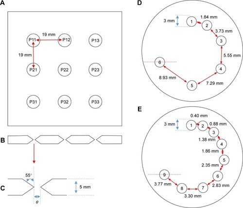
The MC model, as outlined in Figure 1, was developed using the Geant4 toolkit (Release 10.04). Source spectra (shown in Figure 2A), which was used directly as a fan beam in the simulations, was generated in advance by using electrons (125 kVp) to hit the tungsten target. The source was filtered by a 0.8 mm thick beryllium window and a 1.8 mm thick tin foil.¹⁶ A polymethyl methacrylate (PMMA) phantom was scanned 15 cm away from source. Detectors were placed at 90° with respect to the incident beam axis and 10 cm away from the phantom. The detector included a 263×263 crystal whose size was 0.25×0.25 mm and the center-to-center distance was 0.45 mm. A multi-pinhole collimator (Figure 3A–C), which consisted of a 5 mm thick lead plate and nine pinholes (aligned in three rows containing three pinholes each) was placed between the phantom and the detector. The pinhole was designed to have a cone-shaped profile with an acceptance angle of 110°, which was selected to cover the object; its center-to-center distance was 1.9 cm, which was chosen to avoid projection overlaps.

Figure 1 Schematic for the current MC model with the system components.

Note: The red arrows signify the emission of XRF photons from the phantom, which strike the detectors.

Abbreviations: MC, Monte Carlo; XRF, X-ray fluorescence.

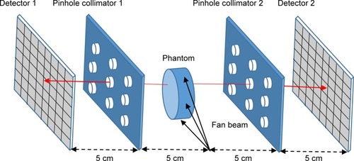
Figure 2 (A) Source spectra and (B) XRF and scattered photon spectrum.

Notes: The XRF and scattered photon spectrum were measured from the crystal positioned at the 69th row (from top) and the 128th column (from left); the multi-pinhole size was 3.7 mm. The red line is a third order polynomial fit of the spectrum from 50 keV to 100 keV.

Abbreviation: XRF, X-ray fluorescence.

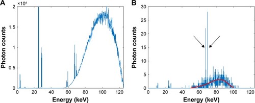
Figure 3 Layout of multi-pinhole collimator and PMMA phantoms.

Notes: (A) Perpendicular view of the lead plate containing nine pinholes; (B) cross-section of the lead plate containing the centers of the pinholes; (C) cross-section of a pinhole; (D) phantom with six inserts and (E) phantom with nine inserts.

Abbreviation: PMMA, polymethyl methacrylate.

Phantoms

Three PMMA phantoms (3 cm in diameter, 0.5 cm in height) were used in the simulations: 1) phantom (I) (Figure 3D) contained six GNPs inserts (1 wt.% concentration) with adjacent separations of 1.84, 3.73, 5.55, 7.29 and 8.93 mm; 2) phantom (II) (Figure 3E) contained nine GNPs inserts (1 wt.% concentration) with adjacent separations of 0.40, 0.88, 1.38, 1.86, 2.35, 2.83, 3.30 and 3.77 mm; and 3) phantom (III) (Figure 3D) contained six inserts with various concentrations of GNPs (1, 0.5, 0.3, 0.2, 0.1 and 0.08 wt.%). All the inserts were designed with a 3 mm diameter and a radial distance of 1 cm.

Data acquisition and processing

The MC simulations were performed in a multi-thread mode using the high-performance computing cluster at The University of Texas MD Anderson Cancer Center. Twenty to 100 billion photons were used in the simulations. The particle interactions and transportations were modeled using the Penelope low energy electromagnetic physics list, which included photon transport, the photoelectric effect, Compton scattering and Rayleigh scattering.

The central layers of the phantoms were scanned. For a fixed photon number (100 billion), the changed pinhole diameters in the simulations being 1, 2 and 3.7 mm for phantom (I) scans; 1, 0.5 and 0.25 mm for phantom (II) scans and 1 and 2 mm for phantom (III) scans. Only detector 1 was used (one-sided detector) for these simulations. For phantom (II), a pinhole diameter of 1 mm was tested with both detectors 1 and 2 being used (two-sided detector). There was a 0.95 mm offset between the centers of detector 1 and 2 and the scan was performed with 100 billion photons. The photon number was then reduced to 20, 40 and 80 billion to do the simulations without offset. The crystals recorded all photon information (energy and counts), which passed through them. Figure 2B shows the XRF and scattered photon spectrum measured from the crystal positioned at the 69th row (from top) and the 128th column (from left), the multi-pinhole size being 3.7 mm. A third order polynomial (a built-in function of MATLAB, the fitting formula was p(x) = p₁x³ + p₂x² + p₃x + p₄) was fitted from 50 to 100 keV to estimate the Compton background (the red line in Figure 2B). The XRF signal (67.0 and 68.8 keV) was extracted by calculating the difference between the measured signal (indicated by the black arrow in Figure 2B) and the polynomial fit. The projection, which could be divided into nine sub-projections and was related to each of the nine pinholes, was acquired by extracting the XRF signal intensity from each crystal. Only one projection (no rotation) was obtained in all simulations. The image could be reconstructed from the whole projection or from each sub-projection.

For all simulations, the maximum-likelihood expectation maximization (MLEM)^8,21,22 was used to do the reconstructions:

$f_i^{m+1}=\frac{f_i^{m+1}}{{\displaystyle {\sum }_j{M}_{i,j}}}\times {\displaystyle {\sum }_j{M}_{i,j}}\frac{p_j}{{\displaystyle {\sum }_j{M}_{i,j}{f}_i^m}}$(1)

where $f_i^m$ is the ith pixel intensity of the reconstructed image f in the mth iteration. p_j is the element of projection p and describes the XRF signal detected by the jth detector. M_i,j is the element of the system matrix M and represents the probability that a fluorescence photon will be created by the pixel f_i and detected in the projection element p_j. The attenuation correction based on an apriori attenuation coefficient of PMMA²³ at the intensity-weighted mean energy of the excitation beam (85 keV) and at an XRF photon energy (68 keV) was used to build the system matrix:

$M_{i,j}=\frac{\exp (-{\displaystyle {\int }_A^B{\mu }_{beam(l_1)}d{l}_1})exp(-{\displaystyle {\int }_A^C{\mu }_{gold(l_2)}d{l}_2})}{{\left|d\right|}^2}$(2)

where μ_beam and μ_gold are the respective attenuation coefficients of the source photons and the gold K_α photons. l₁ is the segment of the entering object point A toward pixel point B and l₂ is the segment of pixel point B toward exiting object point C. d is the distance from the pixel point B to the detector.

For ease of visual comparison of the reconstructed images, the pixel size was reduced from 0.45×0.45 mm to 0.225×0.225 mm using bilinear interpolation (a built-in function of MATLAB).

Image analysis

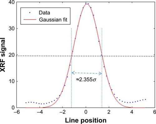
The FWHM¹⁷ was calculated along the red dash lines indicated in Figure 3D and E to compare the spatial resolution of phantom (I) and (II), respectively. Figure 4 shows the Gaussian fit to the line in phantom (I) (the multi-pinhole size is 1 mm), where the FWHM was calculated as 2.355σ (σ is the SD of the fitting Gaussian function).

Figure 4 FWHM of phantom (I) with 1 mm multi-pinhole size.

Abbreviations: FWHM, full-width-at-half-maximum; XRF, X-ray fluorescence.

The CNR^18,19 was determined by calculating the ratio of the difference between the mean values of each region of interest (ROI) with the background and the SD of the background:

$CNR=\frac{{\overline{\overrightarrow{f}}}_{ROI}-{\overline{\overrightarrow{f}}}_{BK}}{\sqrt{{\sigma }^{2}BK}}$(3)

where ${\overline{\overrightarrow{f}}}_{ROI}$ and ${\overline{\overrightarrow{f}}}_{BK}$ are the mean values of the ROI and the background, respectively, and σ_BK is the standard variance of the background.

The LOD was calculated by using the following equation:

$LOD={\overline{\overrightarrow{f}}}_{BK}+3.29{\sigma }_{BK}$(4)

Results

Comparison of multi-pinholes of different sizes

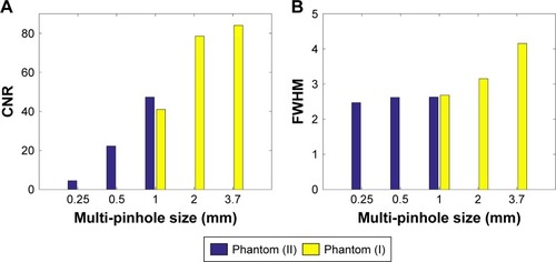
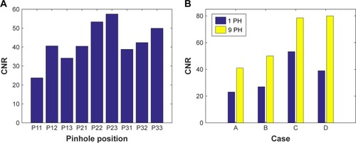
Figure 5 shows the reconstructed images for phantom (I) and (II) with various sizes of multi-pinhole, and Figure 6 presents the corresponding CNR (Figure 6A) and FWHM (Figure 6B). For phantom (I), the resolution (FWHM) increased with decrease in size of multi-pinhole, but noise increased so that the CNR decreased. Inserts 2 and 3 (labels shown in Figure 3D) in the reconstructed image with a 3.7 mm multi-pinhole were connected, whereas the inserts with a 2 mm multi-pinhole were separated. Inserts 1 and 2 in the reconstructed image with a 2 mm multi-pinhole size were connected, whereas the inserts with a 1 mm multi-pinhole were separated. The resolution of the system using the 2 mm multi-pinhole was between 1.84 and 3.73 mm, while that at 3.7 mm was between 3.73 and 5.55 mm. For phantom (II), the resolution (FWHM) remained the same for images formed for the three different sizes of multi-pinhole; inserts 3 and 4 (labels shown in Figure 3E) were separated, whereas inserts 1, 2 and 3 were connected. The resolution of this system with a 1 mm multi-pinhole was between 0.88 and 1.38 mm. Meanwhile, the CNR decreased with decrease in size of multi-pinhole. As expected, reconstructions for phantom (I) and (II) with a 1 mm multi-pinhole gave almost the same CNR and FWHM.

Figure 5 Reconstructed images of (upper) phantom (I) and (lower) phantom (II) with (A) 3.7 mm, (B) 2 mm, (C and D) 1 mm, (E) 0.5 mm and (F) 0.25 mm multi-pinhole. Note: Results are shown for the XFCT setup with 100 billion particles and a one-sided detector.

Abbreviation: XFCT, X-ray fluorescence computed tomography.

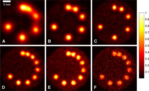
Figure 6 (A) CNR and (B) FWHM of reconstructed images in Figure 5.

Abbreviations: CNR, contrast-to-noise ratio; FWHM, full-width-at-half-maximum.

Comparison of single pinholes and multi-pinholes

Figure 7 depicts the projection of phantom (I) with a 2 mm multi-pinhole. The channels corresponding to the individual pinholes (labels shown in Figure 3A) are clearly separated, and the images do not overlap. The projection shows the structure for a two-dimensional (2D) slice, but the image is noisy and the resolution is poor. Figure 8 presents images that were reconstructed from individual sub-projections in Figure 7, and the image quality would seem to depend on the pinhole position. Figure 9A shows the corresponding CNR, which demonstrates that the CNR depends on the pinhole position.

Figure 7 Projection for phantom (I).

Note: Results are shown for the XFCT setup with a multi-pinhole size of 2 mm, 100 billion particles and a one-sided detector.

Abbreviation: XFCT, X-ray fluorescence computed tomography.

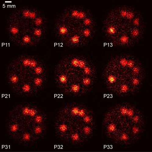
Figure 8 Reconstructed images for phantom (I) acquired using individual sub-projections.

Note: Results are shown for the XFCT setup with a multi-pinhole size of 2 mm, 100 billion particles and a one-sided detector.

Abbreviation: XFCT, X-ray fluorescence computed tomography.

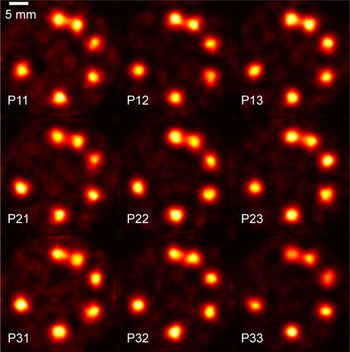
Figure 9 CNR of reconstructed images in (A) Figure 8 and (B) Figure 10.

Abbreviation: CNR, contrast-to-noise ratio.

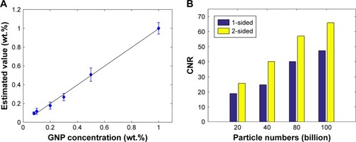
Reconstructed images of phantom (I) and (III) and the corresponding CNRs with different numbers of pinhole are shown in Figures 9B and 10, respectively. As expected, for a given pinhole size, resolution remained the same, while noise increased with decreasing number of pinholes. As shown in Figure 10B and D, the 0.08 wt.% regions are not clearly visible in the images for the nine pinholes’ configurations using both the 1 and 2 mm apertures; however, the 0.08 wt.% and the 0.1 wt.% regions are not clearly visible when the number of pinholes is reduced to 1. In Figure 11A the average estimated concentration of GNPs in the individual GNP regions is plotted against the actual GNP concentrations for the multi-pinhole in Figure 10B. The relationship between the estimated and actual values is sufficiently linear. Table 1 lists the LOD values as presented in Figure 10B and D. The LOD remained the same for different pinhole diameters, while the LOD values were affected by the number of pinholes (~0.13 wt.% for single pinhole and ~0.09 wt.% for nine pinholes). Overall, the results for the nine-pinhole configurations were much better (higher CNR, lower LOD and less artifacts) than that for a single pinhole.

Table 1 LOD (wt.%) for single pinhole and multi-pinhole configurations with different diameters

	1 PH	9 PH
1 mm	0.132	0.088
2 mm	0.129	0.085

Note: Results are shown for the XFCT setup with Phantom (III), 100 billion particles and one-sided detector.

Abbreviations: LOD, limit of detection; PH, pinhole; XFCT, X-ray fluorescence computed tomography.

Figure 10 Reconstructed images for single pinhole and multi-pinhole configurations.

Notes: (A) Phantom (I) with multi-pinhole size of 1 mm, (B) phantom (III) with multi-pinhole size of 1 mm, (C) phantom (I) with multi-pinhole size of 2 mm and (D) phantom (III) with multi-pinhole size of 2 mm employing (upper) one pinhole in the center and (lower) nine pinholes. Results are shown for the XFCT setup with 100 billion particles and one-sided detector.

Abbreviation: XFCT, X-ray fluorescence computed tomography.

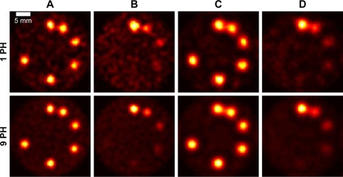
Figure 11 (A) Relationship between the concentration of GNPs estimated using multi-pinhole XFCT (1 mm diameter) and the actual concentration of GNPs by phantom (III), (B) CNR of reconstructed images in Figure 12.

Abbreviations: GNP, gold nanoparticle; XFCT, X-ray fluorescence computed tomography; CNR, contrast-to-noise ratio.

Comparison for different numbers of particles

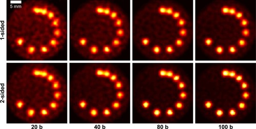
Further studies were then performed for the two-sided detector. Data for the offset configuration and 100 billion particles were reconstructed, and it was found that the resolution of the system was essentially the same as that for the one-sided detector. Figure 12 shows the reconstructed images for phantom (II) with different numbers of particles, and Figure 11B presents the corresponding CNR. As expected, image quality and CNR decreased with a decrease in the numbers of particles. The results for the two-sided detector with 20 and 40 billion particles were the same as those using the one-sided detector with 40 and 80 billion photons, respectively.

Figure 12 Reconstructed images for Phantom (II) obtained using (upper) one-sided and (lower) two-sided detectors with 20, 40, 80 and 100 billion particles.

Note: Results are shown for the XFCT setup with multi-pinhole size of 1 mm.

Abbreviations: b, billion; XFCT, X-ray fluorescence computed tomography.

Discussion

It has been shown that a multi-pinhole benchtop XFCT imaging system can acquire data efficiently and may be feasible for imaging and quantification of GNP-loaded PMMA phantoms. The trade-off between pinhole size and photon counts was investigated, and the performance in the simulations of different sizes of multi-pinhole and different concentrations of GNPs was evaluated. The larger size of multi-pinhole acquired more photon counts but at the same time negatively impacted image resolution, while a smaller size of multi-pinhole ensured higher image resolution but suffered from a lower intensity XRF signal and hence more particles would be needed, which would result in an increased dosage. The image resolution (FWHM) was between 0.88 and 1.38 mm, 1.84 and 3.73 mm, and 3.73 and 5.55 mm for 1, 2 and 3.7 mm sized multi-pinholes, respectively, which clearly approximates to the corresponding multi-pinhole sizes. Image resolution was affected by both the size of the multi-pinhole and the crystal center-to-center distance. The crystal center-to-center distance was 0.45 mm in the simulations, and setting the multi-pinhole size to less than 0.45 mm could not increase the resolution. This fact was supported quantitatively by the results for the 1 mm, 0.5 mm and 0.25 mm multi-pinhole sizes as shown in Figure 6B, whose FWHMs were almost the same.

In Figure 8, the background regions for P11, P21, P31, P13, P23 and P33 were noisier than those of the other pinholes, and this can be explained in terms of X-ray scattering, primarily Compton scattering.

According to a previous study,¹⁶ the CdTe response function could be used to match experimental data with the Geant4 simulated data. In order to save simulation time, the present simulations substituted air for the crystal material and recorded the photons that passed through the crystal. Other detector response functions could be investigated to match the experimental data with the simulated data when the crystal material is not CdTe. This issue is outside the scope of the current study but may be investigated in the future.

Simulations with different numbers of photon particles were compared and results showed that image quality would be less noisy with more photon particles (or dose), which provides a solution to the trade-off between dose/number of photon particles and image quality. One-sided and two-sided detections were compared and results indicated that the two-sided detector could obtain the same image quality as the one-sided detector by using half the number of photon particles.

The current multi-pinhole system can provide a projection (direct 2D slice image) of the object without rotation, and the projection displayed the structure of the 2D slice of the object. However, the size of the multi-pinhole is not small enough to obtain point-to-point information between the 2D slice of the object and the projection. An iterative reconstruction algorithm based on system information was used in the present study to obtain a more accurate structure (less noisy and higher resolution) than the projection. The current multi-pinhole configuration could acquire 3D images by scanning the object layers sequentially. In the future, a cone beam and other multi-pinhole modes¹⁴ could be evaluated in further simulations.

Conclusion

A Geant4-based MC model of a benchtop multi-pinhole XFCT system has been developed and validated. The image resolution of multi-pinhole system with different sizes of multi-pinhole was tested and the performances of multi-pinhole and single pinhole systems were compared. For a PMMA phantom, image resolution between 0.88 and 1.38 mm was obtained for a multi-pinhole of 1 mm, and the multi-pinhole configuration had a higher CNR and fewer artifacts than that of a single pinhole. The multi-pinhole XFCT system could detect a concentration of GNPs in solution of about 0.09 wt.%, which is lower than that for the single pinhole configuration (about 0.13 wt.%). The Geant4-based MC technique has potential for use in a multi-pinhole configuration with polychromatic X-rays and will be used to optimize experimental setups for future development of a multi-pinhole XFCT system.

Acknowledgments

This work was supported in part by the National Natural Science Foundation of China (grant no 61401049) and the Fundamental Research Funds for the Central Universities (grant nos 2018CDGFGD0008 and 10611CDJXZ238826) and the China Scholarship Council.

Disclosure

The authors report no conflicts of interest in this work.