Spatio-temporal variability of CO and O₃ in Hyderabad (17°N, 78°E), central India, based on MOZAIC and TES observations and WRF-Chem and MOZART-4 models

Abstract

This article is based on the study of the seasonal and interannual variability of carbon monoxide (CO) and ozone (O₃) at different altitudes of the troposphere over Hyderabad, India, during 2006–2010 using Measurement of OZone and water vapour by Airbus In-Service Aircraft (MOZAIC) and observation from Tropospheric Emission Spectrometer (TES) aboard NASA's Aura satellite. The MOZAIC observations show maximum seasonal variability in both CO and O₃ during winter and pre-monsoon season, with CO in the range (100–200)±13 ppbv and O₃ in the range (50–70)±9 ppbv. The time-series of MOZAIC data shows a significant increase of 4.2±1.3 % in the surface CO and 6.7±1.3 % in the surface O₃ during 2006–2010 in Hyderabad. From MOZAIC observations, we identify CO and O₃ profiles that are anomalous with respect to the monthly mean and compare those with Weather Research Forecast model coupled with Chemistry (WRF-Chem) and Model for OZone and Related Tracers, version 4 profiles for the same day. The anomalous profiles of WRF-Chem are simulated using three convection schemes. The goodness of comparison depends on the convection scheme and the altitude region of the troposphere.

• MOZAIC
• WRF-Chem
• CO
• O₃

1. Introduction

CO and O₃ are trace gases that play a very important role in the Earth's atmospheric chemistry. CO is important in the context of climate change, as it indirectly affects the radiative forcing by affecting concentrations of greenhouse gases such as O₃ and methane (CH₄) (Wigley et al., 2002). In the troposphere, O₃ is a greenhouse gas because of strong absorption of infrared (IR) radiation centred at 9.6 µm and hence contributes to global warming (Gauss et al., 2003).

O₃ is formed in the troposphere through photochemical reactions in the presence of precursors, which include nitrogen oxides (NO_x≡NO+NO₂), CO and volatile organiccompounds (VOCs). The major sources of emission of NO_x are biomass burning, biogenic sources, fossil fuel combustion and lightning (Sauvage et al., 2007; Monks et al., 2009). In addition to this, many anthropogenic activities such as combustion of biofuels, fossil fuels and biomass burning contribute to the emissions of CO, CH₄, NO_x and VOCs in Asia (Cooper et al., 2010; Lamarque et al., 2010; Sahu, 2012). The major loss of tropospheric O₃ is due to the photolysis followed by reaction with water vapour (H₂O). The lifetime of O₃ varies from days to months in the troposphere (Wang et al., 1998; Law, 2010). The metastable oxygen, O(¹D), created by O₃ photolysis, reacts with H₂O and produces OH radicals: This reaction is considered as one of the major sources of OH in the atmosphere. In troposphere, the OH radicals react with CO, CH₄ and VOCs (Fishman et al., 1979), thereby controlling pollution in the troposphere.

The major sources of atmospheric CO include incomplete combustion of fossil fuels and biomass burning (Khalil and Rasmussen, 1994; Holloway et al., 2000; Seinfeld and Pandis, 2006; Duncan et al., 2007). The lifetime of atmospheric CO ranges from weeks to months (Duncan et al., 2007) and thus has an important impact on regional and global air quality as a pollutant which can affect remote regions of the atmosphere (Srivastava and Sheel, 2013).

Various emission inventories have been developed to estimate the contributions of the major sources of CO (Granier et al., 2011). The estimated range of anthropogenic emission among these inventories ranged from 500 to 600 Tg/yr in 2000, with a negative global trend of about 4 % for the last decade (2000–2010) as estimated by the Monitoring Atmospheric Composition and Climate CityZen (MACCity) inventory (Granier et al., 2011). The emissions calculated by this inventory are based on a projection of the future emissions RCP8.5, corresponding to a radiative forcing of 8.5°W in 2100. An increasing trend is found in most of these emission inventories in the regional budget of CO for China and India due to the rapid urbanisation and industrial growth (Ohara et al., 2007; Granier et al., 2011). In India, an increment of about 50–80 Tg/yr has been estimated in anthropogenic CO emissions for the period 1998–2010 (Granier et al., 2011).

Long-term measurements of CO have helped to characterise the spatial and temporal variability and estimate the global and regional budget of CO (Emmons et al., 2000; Duncan et al., 2007). Such measurements are however sparse over South Asia, where long-term vertical profile measurements of CO are crucial to study the effect of long-range transport on the seasonality and interannual variability of CO in the free troposphere (Sheel et al., 2014). Such measurements are available from satellite-based instruments (Worden et al., 2013), which, however, have low resolution and accuracy in the lower troposphere. Thus, vertical profile observations from MOZAIC are valuable. Earlier, we highlighted the roles of long-range transport and biomass burning in the distribution of O₃ and CO over Bangkok using MOZAIC observations (Sahu et al., 2013). Based on MOZAIC observations and models, we have also seen that in Hyderabad, the Planetary Boundary Layer (PBL) CO is predominantly influenced by strong winds from adjoining regions and by elevated local emissions (Sheel et al., 2014). In the free troposphere, we found the seasonal variability was affected by long-range transport associated with the Intertropical Convergence Zone and biomass burning. The interannual variations were mainly due to transition from El Niño to La Niña conditions (Sheel et al., 2014).

In this work, we analyse the vertical profiles of CO and O₃ from MOZAIC and TES observations in Hyderabad with an objective to study the seasonal and interannual variability during 2006–2010. We then compare the observations with the profiles simulated by Weather Research Forecast model coupled with Chemistry (WRF-Chem) and Model for OZone and Related Tracers (MOZART)-4 (Model for OZone And Related Tracers) models.

2. Description of site and local meteorology

Hyderabad (17°27′N and 78°28′E) is situated in the southern peninsular state of Andhra Pradesh in India. The city covers an area of 625 km² with a height of around 545 m above the mean sea level. Hyderabad is the fifth largest city of India, with a population of about seven million people (2011 census). Rapid urbanisation in conjunction with industrialisation has encouraged migration into this city, leading to increasing trend in the number of vehicles as well as industries. Hyderabad has the third largest bus station facility in Asia, with 72 platforms for 89 buses to transport passengers at a time. The number of vehicles in the city reached 2.4 million (www.hyderabad.trafficpolice.co.in/) by March 2011.

An increase in a high-capacity coal thermal power plant in Hyderabad and the increased number of vehicles are the main factors of trace gases emissions: mainly CO (www.appcb.ap.nic.in) and NO_x emissions (Prasad et al., 2006, 2011; Gummeneni et al., 2011). The city is influenced by urban emissions and also by the surrounding rural and suburban regions biomass burning transport.

Hyderabad has a tropical wet and dry climate, with a mixture of wet and dry weather during the hot pre-monsoon period from March to May, the monsoon season from June to September with a total rainfall of about 800 mm, a post-monsoon season (October and November) with well-balanced weather and a dry winter (December to February).

The daily mean surface temperature in Hyderabad varies from a minimum of typically 15 °C in December to a maximum of about 35 °C in May and is rarely beyond these two extremes (Sheel et al., 2014). The temperature does not exhibit any significant interannual variation.

3. WRF-Chem model

In the present study, version 3.2 of the WRF-Chem model is used for the simulation of CO and O₃ in Hyderabad. The model domain is centred at 17°N, 78°E (Hyderabad) and covers South India at 15 km spatial resolution with 50 grid points in both east–west and north–south directions.

The WRF model is a mesoscale non-hydrostatic meteorological model that includes several options for the parameterisations of PBL, land surface and cloud processes (www.wrf-model.org).

Anthropogenic emissions of CO, NO_x, SO₂, non-methane volatile organic compounds (NMVOC), PM10, PM2.5, BC and OC are taken from the Reanalysis of Tropospheric Chemical Composition (RETRO) [http://www.retro.enes.org/index.shtml, Schultz et al. (2007)] and the Emissions Database for Global Atmospheric Research (EDGAR)v4 (http://edgar.jrc.ec.europa.eu, year: 1970–2005) database. The RETRO emissions are representative of the year 2000. EDGAR v4 provides global anthropogenic emissions of greenhouse gases and air pollutants by country. The biogenic emissions of trace species are calculated using the Model of Emissions of the Gases and Aerosols from Nature (MEGAN) (Guenther et al., 2006).

The initial and boundary conditions for the chemical species are updated every 6 h, based on MOZART-4 (Emmons et al., 2010). The physics included for the WRF-Chem run are: the Noah Land Surface Model (Chen and Dudhia, 2001), the Mellor-Yamada Nakanishi-Niino boundary layer scheme (Nakanishi and Niino, 2006), WRF single-moment (wind speedM) 5-class scheme, the Goddard shortwave radiation scheme (Chou et al., 1998) and the rapid radiative transfer model (RRTM) long-wave radiation scheme (Mlawer et al., 1997). The gas-phase chemistry model used is the Regional Acid Deposition Model, version 2 (RADM2) (Stockwell et al., 1990) which includes 57 chemical species and 158 gas-phase reactions, of which 21 are photolytic. The Secondary Organic Aerosol Model (SORGAM) (Schell et al., 2001) for the carbonaceous secondary fraction.

We perform the simulation with Mellor–Yamada–Janjić (MYJ) PBL scheme (Janjić, 1990) and three different cumulus parameterisation schemes: Kain–Fritsch (Kain and Fritsch, 1990; Kain, 2004), Betts–Miller–Janjić (Betts and Miller, 1986) and Grell–Dévényi (Grell and Dévényi, 2002) ensembles.

4. MOZART (version 4)

In the present work, we use version 4 of MOZART. It is an off-line three-dimensional global chemical transport model which includes comprehensive tropospheric chemistry, simulating 85 gas-phase species, 12 bulk aerosol species, 157 gas-phase and 39 photolysis reactions (Emmons et al., 2010; Srivastava and Sheel, 2013).

MOZART-4 model diagnoses convective mass fluxes using the shallow and mid-level convective transport formulation of Hack et al. (1994) and deep convection scheme of Zhang and MacFarlane (1995). The boundary layer vertical diffusion is based on the parameterisation of Holstlag and Boville (1993). Brasseur et al. (1998) formulation is taken for wet deposition. Advective transport as described in Horowitz et al. (2003) incorporates the flux-form semi-Lagrangian transport algorithm of Lin and Rood (1996).

The simulation from MOZART-4 for this work is driven by meteorological fields from the NASA GMAO GEOS-5 model. These anthropogenic emissions are based on David Streets’ inventory (www.cgrer.uiowa.edu/arctas/emission.html) for ARCTAS and fire emissions from FINN-v1 (Wiedinmyer et al., 2011). These results are at 1.9×2.5 degrees with 56 levels.

5. Observations

5.1. MOZAIC

The MOZAIC provides in situ observation of vertical atmospheric profiles of CO and O₃ along with the simultaneous observations of meteorological parameters such as relative humidity (RH), wind speed, wind direction and temperature. The MOZAIC Project was initiated in 1993 to study the variability of the chemical composition in the atmosphere (Marenco et al., 1998).

For the measurement of CO, a Thermo Environmental Instrument (Model 48CTL) based on the gas filter correlation technique was used. The IR radiation absorption at a wavelength of 4.67µm was used for the detection of CO. MOZAIC has measurement precision of ±5 ppbv (signal noise), ±5 % (calibration) and minimum detection limit of 10 ppbv were achieved for a 30-s integration time.

A dual-beam ultraviolet absorption instrument from Thermo-Electron (Model 49–103) having a detection limit of 2 ppbv is used to perform the O₃ measurement. The upper limit of the estimated error in measurement was to be ±(2.0 ppbv+2 %) (Thouret et al., 1998a, b). Thouret et al. (1998b) provides a detailed description of O₃ sampling procedure, measurement technique, calibration, instrument validation and quality testing.

The flight observations provide the vertical profile data during both take-off and landing of the aircraft. CO and O₃ measurements are taken every 30 s from take-off to landing. Raw data (30 s time resolution) are averaged over 150 m height intervals. Profiles are defined as the part of the flight between ground level and the first pressure-stabilised cruising level, usually up to about 300 hPa (200 hPa) with regard to the ascent (descent) profile. Thus, the profile data extend to a maximum of 12 km altitude, due to the predefined cruise altitude by international air traffic regulations. The measuring aircraft does not ascend/descend vertically above a location but that it follows a well-defined flight path before reaching cruise altitude. Below about 4 km, this may not be far from the city, but at higher altitudes, it may extend horizontally to some 200 km from the destination.

5.2. TES/AURA data for O₃ and CO

The TES was launched in July 2004 aboard the Earth Observing System (EOS) Aura satellite. Data were obtained from Giovanni online data system, developed and maintained by the NASA Goddard Earth Sciences Data and Information Services Center (GES DISC). TES is nadir viewing in a polar-orbiting Sun-synchronous orbit with a local crossing time of 01:45 and 13:45 (Zhang et al., 2010). TES has a vertical resolution of approximately 6 km with a high sensitivity between 700 hPa and 300 hPa (Worden et al., 2004). We use available data for the period covering 2006–2010 in this study. The level three data used were pre-processed and all negative values were filtered out. Previous comparisons with in situ measurements show that TES has a positive bias of 5.3 ppbv for O₃ at 500 hPa (Zhang et al., 2010). In the case of CO, the TES CO retrievals have been found to be consistent with those from MOPITT (Luo et al., 2007a) and within 15 % of aircraft data (Luo et al., 2007b; Lopez et al., 2008).

6. Methodology

In this section we discuss the methodologies adopted to evaluate the TES observations and model simulations with respect to MOZAIC in situ observations. To assess the comparison between model simulation and observation we have calculated the mean bias by taking MOZAIC observations as a reference. The formula used here to calculate the mean bias is as follows:1 where o_i and m_i represent the observed and modelled species concentrations, respectively. N is the total number of data pairs. The MOZAIC CO and O₃ observed profiles are interpolated to those altitudes at which TES, WRF-Chem and MOZART-4 profiles are available. The mean bias is calculated for different altitude regions of the troposphere by dividing it into distinct layers (0–2, 2–4, 4–6, 6–8 and 8–10 km).

We have studied interannual variability at different tropospheric altitude regions by subtracting the climatological CO and O₃ amount (hereafter we refer it as SM) from corresponding monthly mean (MM) of CO and O₃ yielding monthly mean anomalies (MMA) (Petropavlovskikh et al., 2005) such as:2 Here, the climatology is computed as mean value of both CO and O₃ data selected for each of the 12 calendar months over the entire 2006–2010 period. This method provides adequate information for analysis of long-term CO and O₃ changes and anomalies (departures from the mean) by accounting empirically for seasonal oscillations in the data. The interannual changes in CO and O₃ from TES and MOZAIC observations are estimated using linear regression model followed by a p value test against the significance level (α) of 0.05 (Piegorsch, 2002). The p≤0.05 is generally interpreted as statistically significant.

7. Results and discussion

The in situ observations of MOZAIC provide very accurate measurement of atmospheric CO, O₃ and meteorological parameters such as temperature, water vapour mixing ratio, wind speed and wind direction. This offers an opportunity to study the seasonal, interannual variability as well as the various scientific aspects of chemical transport models to predict the concentration of the atmospheric chemical species.

We have analysed 5 years of MOZAIC in situ data in Hyderabad from 2006 to 2010 with approximately more than 800 total observations. In this section, we discuss the seasonal and interannual variability of CO and O₃ in Hyderabad based on MOZAIC and TES observations. The TES observations are evaluated with respect to MOZAIC data in terms of mean bias and vertical resolution. We also discuss the CO and O₃ profiles simulated from WRF-Chem and MOZART-4 model in comparison to MOZAIC observations and uncertainties associated with them. The year 2009 is chosen for this study, since in this particular year, we have more number of MOZAIC observations compared to other years.

7.1. Seasonal and interannual variability

7.1.1. Seasonal variability based on MOZAIC and TES observations

The average CO and O₃ profiles obtained from MOZAIC measurements and TES observations for the period 2006–2010 in Hyderabad for four seasons are shown in Figs. 1 and 2. The seasons are namely December, January, February (DJF); March, April, May (MAM); June, July, August (JJA); and September, October, November (SON). It may be noted from the MOZAIC monthly average profiles in Fig. 1 that the variation in CO concentration is 100–200, 100–180, 100–110 and 100–140 ppbv, respectively, in DJF, MAM, JJA and SON with an average standard deviation of ~±13 ppbv throughout the troposphere. However, the variation in O₃ concentration (Fig. 2) is ~50, 60–70, 30–50 and 40–50 ppbv, respectively, in DJF, MAM, JJA and SON with all having an average deviation of ~±9 ppbv throughout the troposphere. The high value of CO in DJF and MAM season is due to the heavy biomass burning that comes out from forest fires and crop burning (agricultural fires) during this period of time (Venkataraman et al., 2006), which is also resulting in the high value of O₃ during the same period as CO being one of its precursor.

Fig. 1 Mean vertical profiles of CO of MOZAIC and TES observations are plotted along with standard deviation for different seasons (DJF, MAM, JJA and SON) during a 5-yr period (2006–2010). N represents the total number of profiles.

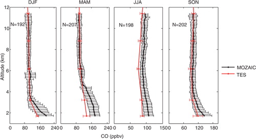
Fig. 2 Mean vertical profiles of O₃ of MOZAIC and TES observations are plotted along with standard deviation for different seasons (DJF, MAM, JJA and SON) during a 5-yr period (2006–2010). N represents the total number of profiles.

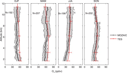
The average profiles of CO and O₃ retrieved from TES observations are also shown in Figs. 1 and 2. CO and O₃ obtained from TES retrieval are evaluated between 2–8 and 8–10 km altitude region (Table 1). We focus only on 2–8 km altitude region due to high sensitivity of TES between 700 and 300 hPa.

Table 1. Mean bias between TES and MOZAIC observations for four seasons DJF, MAM, JJA and SON is calculated at different tropospheric altitude regions

	Mean bias for CO (ppbv)		Mean bias for O3 (ppbv)
Time	2–8 km	8–10 km	2–8 km	8–10 km
DJF	27.9	0.8	−8.6	−7.0
MAM	31.8	−2.3	−11.0	−0.6
JJA	17.9	10.1	−9.7	−3.1
SON	19.4	2.8	−5.3	3.3

The mean bias is calculated between MOZAIC and TES observation for CO and O₃ using eq. (1) (shown in Table 1).It may be noted from Table 1 that mean bias ranges between 18–32 ppbv for CO and −5 – −11 ppbv for O₃. It may also be noted from Figs. 1 and 2 and Table 1, the vertical profiles of O₃ from TES are much better compared to CO in terms of mean bias and standard deviation. This can be explained on the basis of the two very important measures of retrieval which are total degrees of freedom (DOF) and total bits. Total DOF is the trace of the averaging kernel which may be interpreted as a number of statistically independent elements of the estimate. The total bits indicate the reduction in error volume for the retrievals. Worden et al. (2004) estimated DOF and total bits for TES retrieved CO and O₃ are 0.7, 4.9 and 0.8, 8.5, respectively, which shows the sensitivity of O₃ retrieval better compared to CO. Further, the TES retrieval of O₃ is better in autumn (SON) compared to the other seasons which is due to the least contamination of IR radiance by clouds in this particular season. It is also important to note that in this type of comparison between TES or other space-borne instrument versus aircraft observations, whether fresh plumes and stratospheric influence remains an issue.

7.1.2. Interannual variability based on MOZAIC and TES observations

The interannual variability in CO and O₃ is studied at different tropospheric altitude regions using eq. (2). The MOZAIC observations are used to calculate the changes in CO and O₃ concentration during the 5-yr period in the three different tropospheric layers (0–2, 2–8 and 8–10 km). However, the interannual variability in CO and O₃ concentration from TES observation is studied in 2–8 km region due to high sensitivity of TES in this particular region.

The interannual changes estimated from MOZAIC and TES observations for both CO and O₃ along with the associated standard deviations are given in Figs. 3 and 4 and Table 2. It can be seen from Figs. 3 and 4 that the near-surface (0–2 km) tropospheric CO and O₃ over Hyderabad shows significant increase of 4.3±1.4 and 6.7±1.4 % per annum, respectively, during 2006–2010 with p value 0.003 and 0.0001 respectively. However, in the 2–8 km region, both MOZAIC and TES show a decrease at the rate of −2.0±0.7 and −1.6±0.4 % per annum respectively in CO (Fig. 3) with p value 0.006 and 0.007 respectively, in addition, no significant interannual change is observed in O₃ (Fig. 4) in the same region from both MOZAIC and TES observations. It may also be noted that in the 8–10 km tropospheric layer, no significant decrease is observed for CO (Fig. 3); however O₃ (Fig. 4) shows a decrease with −2.7±0.8 % per annum with p value 0.004.

Fig. 3 Monthly mean anomalies of CO are shown over Hyderabad in the three tropospheric layers with MOZAIC (0–2, 2–8 and 8–10 km) and TES (2–8 km) observations. N and p represent the total number of MOZAIC profiles and p value, respectively.

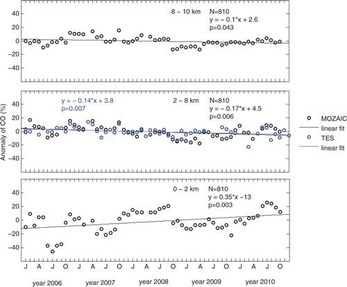
Fig. 4 Monthly mean anomalies of O₃ are shown over Hyderabad in the three tropospheric layers with MOZAIC (0–2, 2–8 and 8–10 km) and TES (2–8 km) observations. N and p represents the total number of MOZAIC profiles and p value, respectively.

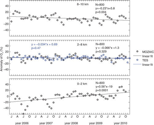
Table 2. Changes in CO and O₃ obtained from MOZAIC observations with respect to the year 2006 in Hyderabad

Hyderabad (17.3°N, 78.4800°E)
Tropospheric Layers (km)	Changes in CO (% with respect to 2006)	Changes in O3 (% with respect to 2006)
0–2	+4.2±1.3	+6.7±1.3
2–8	−2.0 (−1.6)±0.7 (0.4)	−0.7 (0.3)±0.7 (0.4)
8–10	−1.2±0.48	−2.7±0.8

Change in CO and O₃ with TES observations are shown in 2–8 km layer in bracket along with the MOZAIC observations.

Some of the facts that support the in situ observations obtained from MOZAIC in Hyderabad are discussed here. One of the major factor that could lead to an increase in the near-surface level (0–2 km) of CO and O₃ mixing ratios over the Hyderabad is the increase in anthropogenic emissions in the past decade (Beig and Brasseur, 2006; Ghude et al., 2013). Ghude et al. (2013) reported the increase of NO_x emissions by more than approximately 65 % in Hyderabad; however, the world's CO concentration has declined during the same period. It is also interesting to note the reported trends (Granier et al., 2011) from comparing several global and regional emission inventories. They have shown a very slight decrease in global anthropogenic CO emissions (around 1 %) from 1990 to 2010, with larger decreases for Europe and the USA (~3 % yr⁻¹). However, they show increases for India (~1.5 % yr⁻¹) and China (~3 % yr⁻¹) for 2006 to 2010.

Power stations, road transport, industries, use of coal for domestic purposes and burning of fossil fuels are the major sources of air pollution in the city (Gurjar et al., 2004; Kulkarni et al., 2010). It has been found that the urban and vehicular population of Hyderabad was 2.5 and 0.08 million in 1981, whereas in 2011 it has reached up to 6.8 (source: www.iipsenvis.nic.in) and 0.3 million (source: www.mospi.nic.in), respectively. The rapid growth of urban and vehicular pollution in Hyderabad is the result of speedy increase in economic activities after 1990s. In a recent study, Sahu et al. (2014) compared their results with sector-specific estimation as that of Ohara et al. (2007) for 2000. They estimated that the NO_x emission in 2009 was 5.4 Tg yr⁻¹ which is quite high compared to the estimation made for 2000 by Ohara et al. (2007). They studied the Indian on-road emission inventories to check out the emission distribution of each vehicle category and their relative contribution of emission from different technological distributed age groups like 5, 10, 15 and 20 yr, respectively, for the base year 2009. They have shown that the reason behind the increase of NO_x emission was due to the increase in the number of old vehicle (10–20 yr) segment with time. Similarly, it has been shown that the CO estimation of 10.2 Tg yr⁻¹ in 2009 was just 30 % higher than the estimation made for 2000. They argued that the main reason could be due to the rise in personal vehicles as well as two-wheeler segments in recent time. Girach and Nair (2014) have also shown the increasing trend in total CO emission from India over 2000–2008 that were estimated from EDGAR version-4.2 inventory and REAS (Regional Emission inventory in ASia) version-2.1 inventory (Kurokawa et al., 2013).

In the present study, we have also analysed the anthropogenic emission data of CO and NO_x for Hyderabad during 2005–2010 using MACCity global emission inventory (Granier et al., 2011). The MACCity (MACC/CityZen) emission dataset is the extension of the ACCMIP (Atmospheric Chemistry and Climate – Model Intercomparison Project) historical emissions dataset (Lamarque et al., 2010) as well as the RCPs [Representation Concentration Pathways, van Vuuren et al. (2011)] emission dataset for the MACC and CityZEN projects. As part of two projects funded by the European Commission, MACC and CityZen, the ACCMIP and the RCPs emissions dataset have been adapted and extended on a yearly basis for the period 1990–2010. The anthropogenic emission data of MACCity include a lot of sources such as transportation, energy, solvent, waste, industries, residential, agricultural waste, agriculture and ships. It has been found that the CO and NO_x emission in Hyderabad has increased significantly. It was 148 000 tons for CO and 3800 tons for NO_x in 2005, whereas at the end of year 2010 it reached up to 154 000 tons for CO and 4280 tons for NO_x.

7.2. Comparison of MOZAIC profiles with WRF-Chem and MOZART-4 Model Simulation

This study is divided in two parts. Firstly, we analyse the monthly average CO and O₃ vertical profiles from MOZAIC observations, and WRF-Chem and MOZART-4 models for approximately each alternative month of year 2009 (January, March, June, August and November). Secondly, we study the anomalous profiles of CO and O₃ from MOZAIC observations for the months mentioned above and compared with the corresponding temporarily and spatially collocated profiles of WRF-Chem and MOZART-4 models.

7.2.1. Comparison of monthly average profiles of CO and O₃ of MOZAIC with WRF-Chem and MOZART-4 Model Simulation

The monthly average profiles of CO and O₃ observed from MOZAIC observations are analysed by dividing the months into monsoon and pre-monsoon category. We consider January, March and November as pre-monsoon months in general and June and August are considered as monsoon months.

The monthly average variation in CO profiles is shown in Fig. 5. It may be noted from Fig. 5, that CO variation in pre-monsoon and monsoon months ranges (90–270) ±17 ppbv and (100–200) ±15 ppbv, respectively. Figure 6 shows the monthly average variation in O₃ profiles, and it can be seen that the monthly average variation in O₃ concentration in pre-monsoon and monsoon months ranges (30–80) ±11 ppbv and (20–90) ±14 ppbv, respectively.

Fig. 5 Monthly mean profiles of CO along with standard deviation are plotted for different months of the year 2009 for MOZAIC observations and WRF-Chem and MOZART-4 simulations. N represents the total number of profiles of that particular month.

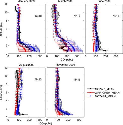
Fig. 6 Monthly mean profiles of O₃ along with standard deviation are plotted for different months of the year 2009 for MOZAIC observations and WRF-Chem and MOZART-4 simulations. N represents the total number of profiles of that particular month.

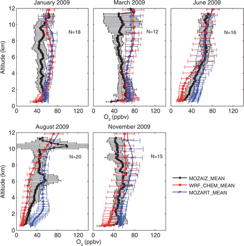
Figure 5 also shows the monthly average profiles simulated from WRF/Chem and MOZART-4 models. We have calculated the mean bias (Table 3) to compare the MOZAIC observed monthly average profiles with those simulated from WRF-Chem and MOZART-4 models using eq. (1). Both the models have reproduced observed variability in CO and O₃ for pre-monsoon and monsoon monthly averaged profiles. It may be noted from Table 3, in the near-surface tropospheric layer (0–2 km), the mean bias in CO between WRF-Chem (MOZART-4) and MOZAIC in pre-monsoon and monsoon monthly average profiles is ~52.5 (35.7) and 46.4 (17.6) ppbv respectively; however, in the mid to the high level of troposphere (2–10 km), it is ~7.2 (6.5) and 16.6 (16.3) ppbv, respectively. Similarly, the mean bias in the near-surface tropospheric layer (0–2 km) in O₃ between WRF-Chem (MOZART-4) and MOZAIC in pre-monsoon and monsoon monthly averaged profiles is ~9.3 (6.1) and 6.4 (11.4) ppbv, respectively; however, in the mid to the high level of troposphere (2–10 km), it is ~13.2 (15.6) and 9.4 (8.2) ppbv, respectively.

Table 3. Mean bias is calculated for monthly average WRF-Chem and MOZART-4 simulated CO and O₃ with respect to MOZAIC observations for different months of the year 2009.

	Mean Bias with WRF-Chem (MOZART-4) for CO (ppbv)
Time	0–2 km	2–4 km	4–6 km	6–8 km	8–10 km
Jan 2009	53.6 (−26.9)	31.0 (−3.7)	7.8 (12.0)	7.0 (6.9)	−4.4 (2.1)
March 2009	−49.6 (−71.7)	−0.9 (−23.2)	5.2 (−1.3)	6.8 (0.5)	2.4 (−2.2)
Jun 2009	49.3 (23.3)	40.7 (11.8)	28.8 (6.2)	17.4 (1.3)	14.1 (5.2)
Aug 2009	43.6 (12.0)	16.8 (−11.4)	9.0 (−28.2)	0.1 (−31.9)	−6.5 (−34.4)
Nov 2009	54.5 (−8.6)	5.1 (−9.8)	4.9 (4.1)	5.9 (5.6)	5.3 (7.4)
	Mean Bias with WRF-Chem (MOZART-4) for O3 (ppbv)
	0–2 km	2–4 km	4–6 km	6–8 km	8–10 km
Jan 2009	3.9 (−3.5)	−12.5 (−11.5)	−19.7 (−17.2)	−21.4 (−20.9)	−10.9 (−15.7)
March 2009	−12.1 (−8.3)	−5.1 (−7.6)	−12.3 (−11.6)	−23.9 (−21.9)	−27.2 (−21.8)
Jun 2009	7.8 (−11.3)	15.0 (−10.7)	7.6 (−6.4)	2.4 (1.5)	1.8 (−0.3)
Aug 2009	5.0 (−11.5)	10.0 (−22.9)	15.8 (−13.0)	20.9 (−2.9)	−1.8 (−8.3)
Nov 2009	11.9 (−6.7)	6.2 (−8.9)	4.6 (−9.9)	−2.9 (−15.5)	−12.6 (−25.7)

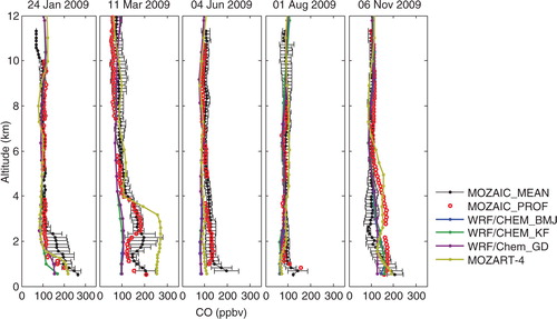
7.2.2. Comparison of anomalous profiles of CO and O₃ of MOZAIC with WRF-Chem and MOZART-4 Model Simulation

In the previous section we have compared the monthly averaged profiles of CO and O₃ of MOZAIC with WRF-Chem and MOZART-4 simulations. We have also extended the simulation study in the case of few anomalous profiles of CO and O₃ that are obtained from MOZAIC observations. We refer these profiles anomalous due to their very high or low value compared to the corresponding monthly average profiles of CO and O₃ of MOZAIC (Figs. 7 and 8). The anomalous profiles are also divided into pre-monsoon and monsoon category. We consider 24 January, 11 March and 6 November 2009 profiles as pre-monsoon profiles and 4 June and 1 August 2009 profiles as monsoon profiles.

Fig. 7 The monthly mean MOZAIC CO profiles (MOZAIC_MEAN) for 5 months of the year 2009 are shown along with the standard deviation. The anomalous profile observed by MOZAIC for a particular month is shown along with the spatially and temporarily collocated profile simulated by WRF-Chem using BMJ, KF and GD convection schemes and MOZART-4 model.

We have calculated the mean bias [eq. (2)] for CO and O₃ simulated from WRF-Chem and MOZART-4; mean bias is also calculated for meteorological variables simulated from WRF-Chem with respect to the MOZAIC observations using eq. (2). In addition, we have calculated the mean bias for CO and O₃ simulated from different convection schemes of WRF-chem model since mesoscale models like WRF-Chem are unable to explicitly resolve convective cloud formation when the grid resolution is coarser than about 10 km. Thus model simulations using grid resolutions of 10 km or larger require parameterisation of cumulus clouds. The goal of cumulus parameterisation is to determine the collective effects of cumulus clouds, rather than to resolve how a single cloud affects the vertical profile (Arakawa and Schubert, 1974). In the present study, simulations with 15 km grid resolution have been compared using three different cumulus parameterisation schemes: Kain-Fritsch, Betts-Miller-Janjić and Grell-Dévényi ensembles that use MYJ PBL scheme for all convection schemes. The MYJ scheme determines eddy diffusion coefficients from prognostically calculated turbulent kinetic energy (TKE) (Hu et al., 2010).

The turbulent diffusion coefficient is diagnosed in MYJ PBL scheme and passed to a separate subroutine to compute the vertical mixing of chemical species. As a result, only local mixing is considered for chemical species while non-local mixing and entrainment processes are not considered for chemical species included in WRF-Chem even though they are considered for meteorological variables.

The KF cumulus parameterisation scheme (Kain and Fritsch, 1990; Kain, 2004) uses the Lagrangian parcel method and satisfies sub-grid scale convection through a mass-flux approach. It involves three important steps. First, it identifies whether instability exists and then determines if existing instability will lead to cloud growth. It then calculates properties of the convective clouds. The accomplishment of these tasks takes place over several steps, first by identifying potential source layers, or updraft source layers (USLs). The second compares the temperature of the environment (T_env) with that of parcel (T_par). If T_par<T_env(negative buoyancy), a temperature perturbation is assigned to the parcel based on the strength of the vertical motion which typically increases T_par by 1–2 K. Again if T_par is still less than T_env, the base of the USL is moved up one model level and the process is repeated. If T_par is warmer than T_env, the parcel is released at its lifting condensation level (LCL) based on its original unperturbed temperature and vertical motion profile. Finally, the KF closure assumption is based on a Convective Available Potential Energy (CAPE) removed process. The updraft and environment mass fluxes are rearranged in the mass column until 90 % of the CAPE over a time period which is typically between 0.5 and 1 h long (Kain, 2004). The removal of CAPE is performed by rearranging the mass in a column using the updraft, downdraft and environmental mass fluxes.

The Betts-Miller-Janjic (BMJ) cumulus parameterisation scheme is the extension of the Betts–Miller scheme (Betts and Miller, 1986). Similar to the KF scheme, BMJ is triggered when a parcel of air ascends a certain distance, as well as having positive CAPE. The BMJ scheme then adjusts the atmospheric temperature and moisture profile toward a reference structure of temperature and moisture profile by using deep and shallow convection. The reference structures are pre-monsoon-determined profiles of temperature and moisture inside the cumulus scheme.

The GD ensemble cumulus parameterisation scheme (Grell and Dévényi, 2002) is ideal for high resolution (ARW WRF User's Guide, 2009). The scheme employs a variety of mass-flux and closure assumptions, feedback assumptions and trigger functions at each grid point; the various closure assumptions include vertical advection of moisture, vertical velocity and CAPE removal, similar to that in KF. The feedback assumptions include perturbations based on cloud size and entrainment strength and detrainment from updrafts. The difference in static control (cloud properties) is combined with differences in dynamic control (the modulation of the convection by the environment) which are based on CAPE, vertical velocity and moisture convergence. Using ensemble and data assimilation techniques, the GD scheme statistically determine the best approach to ingest back to the model.

Table 4 gives the mean bias calculated for CO and O₃ for WRF-Chem (using BMJ, KF and GD convection schemes) and MOZART-4 simulations. In the two pre-monsoon (24 January 2009, 6 November 2009) and one monsoon (4 June 2009) anomalous profiles, WRF-Chem reproduces the observed variability in CO and O₃ throughout the troposphere in good agreement compared to the remaining two anomalous profiles each from pre-monsoon (11 March 2009) and monsoon (1 August 2009). In the 11 March 2009 profile, both the models have large bias in CO (>70 ppbv) in the surface region (0–2 km); however, the KF scheme of WRF-Chem has approximately 6 ppbv less bias in CO in the surface region compared to the MOZART-4 and the other WRF-Chem convection schemes. Furthermore, both the profiles (11 March and 1 August 2009) have large bias in O₃ in the 6–8 km altitude region with all WRF-Chem convection schemes and MOZART-4 model; however, MOZART-4 model has less bias in O₃ in the 11 March 2009 profile at 6–8 km altitude region compared to the WRF-Chem. It may also be noted that in these two anomalous profiles the maximum mean bias with WRF-Chem in O₃ in 6–8 km altitude region is approximately 100 % higher compared to the maximum bias of remaining profiles which is 22 ppbv in 24 January 2009 anomalous profile in 4–6 km altitude region.

Table 4. Mean bias in O (CO) for the anomalous profiles of the year 2009 is calculated at different layers of the troposphere

24 Jan 2009
	WRF-Chem
Altitude (km)	BMJ	KF	GD	MOZART-4
0–2	−5.8 (19.8)	−5.8 (19.8)	−0.2 (5.6)	−7.8 (−14.2)
2–4	−21.8 (19.4)	−21.9 (19.4)	−22.1 (21.5)	−28.6 (17.3)
4–6	−22.7 (3.0)	−22.7 (3.1)	−22.3 (3.0)	−19.1 (0.4)
6–8	−5.6 (9.8)	−5.6 (9.8)	−5.7 (9.5)	−6.5 (4.3)
8–10	−16.3 (3.2)	−16.2 (3.2)	−17.1 (3.7)	−13.9 (10.0)
11 March 2009
0–2	−4.1 (37.8)	−7.0 (37.7)	−6.3 (35.1)	−31.4 (−75.3)
2–4	7.8 (77.0)	8.5 (76.8)	13.1 (70.0)	−20.1 (−76.7)
4–6	−18.7 (13.8)	−23.2 (15.1)	−22.6 (14.3)	−12.2 (−20.3)
6–8	−44.4 (0.1)	−45.4 (0.2)	−45.7 (0.1)	−22.9 (0.1)
8–10	−33.7 (−13.4)	−33.9 (−13.4)	−32.8 (−13.4)	−18.2 (−29.7)
4 June 2009
0–2	5.6 (36.1)	7.3 (34.5)	4.9 (34.0)	−6.9 (20.7)
2–4	5.2 (27.9)	6.9 (26.2)	7.2 (26.6)	−5.1 (19.5)
4–6	0.1 (5.2)	−0.4 (5.1)	−0.8 (5.1)	4.3 (12.0)
6–8	−12.8 (2.2)	−12.3 (2.5)	−10.8 (2.7)	23.3 (6.1)
8–10	−20.6 (13.6)	−19.3 (14.1)	−19.8 (13.3)	0.6 (9.5)
1 Aug 2009
0–2	5.1 (15.7)	6.4 (18.9)	5.7 (15.3)	−2.4 (17.0)
2–4	10.0 (−7.7)	12.1 (−2.1)	13.5 (−3.1)	−9.0 (−8.3)
4–6	16.9 (1.4)	14.1 (3.1)	19.1 (1.6)	10.8 (−10.9)
6–8	38.6 (5.1)	31.0 (7.4)	31.1 (6.6)	32.3 (−23.4)
8–10	14.0 (5.0)	14.3 (6.8)	9.6 (2.2)	4.9 (−2.8)
6 Nov 2009
0–2	−5.3 (16.2)	−9.6 (14.2)	−11.3 (39.7)	−23.6 (16.9)
2–4	6.1 (34.0)	8.8 (30.5)	2.7 (27.9)	−5.4 (11.7)
4–6	−3.0 (25.1)	6.7 (21.5)	−4.4 (24.2)	8.7 (−23.3)
6–8	−7.5 (19.5)	−8.4 (20.0)	−4.4(17.5)	11.3 (3.6)
8–10	4.5 (6.5)	1.7 (9.8)	2.7 (9.4)	−17.6 (17.8)

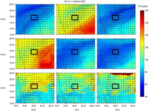
We can explain these two large discrepant profiles (11 March and 1 August 2009) by looking at the meteorological parameters corresponding to them. The meteorology plays a very important role in these profiles since these are at night time (21 GMT) and the advantage of WRF-Chem model is that it simulates meteorological parameters along with the chemical species concentration. The meteorological parameters such as temperature, water vapour mixing ratio, wind speed and wind direction corresponding to all anomalous profiles are simulated with WRF-Chem and compared with the MOZAIC observations (Figs. 9, 10 and 11). Table 5 presents the mean bias calculated for the meteorological parameters at the different regions of the troposphere. It may be noted that the mean bias in temperature, water vapour mixing ratio and wind speed between WRF-Chem simulations and MOZAIC observations varies from 0.0 to 2 K, 0.0 to 4.6 mg/kg and 0 to 6.7 m/s, respectively. Temperature simulations from WRF-Chem model are much more accurate compared to the water vapour mixing ratio, wind speed and wind direction. The WRF-Chem underestimates the water vapour mixing ratio simulation (Fig. 9) in almost each profile. The wind speed simulation (Fig. 10) from WRF-Chem is also in acceptable limit of accuracy except in pre-monsoon profile (11 March 2009) where there is overestimation of wind speed at the level of high troposphere (9–12 km). Figure 11 shows the wind direction plots of WRF-Chem simulations along with MOZAIC observations. It may be noted from Fig. 11 that the uncertainty in WRF-Chem simulation of wind direction is very high between 4 and 6 km altitude region in pre-monsoon profile (11 March 2009). The WRF-Chem simulation shows that the wind direction is north-west and south-west direction (ranging from 225 to 350 degrees) whereas the observations from MOZAIC data show that the wind direction is in north-east direction (ranging from 20 to 80 degrees). In addition, we have also shown the wind direction plots overlaid on O₃ simulation of 6, 12 and 18 ZMT, respectively, of WRF-Chem at 2, 6 and 8 km altitude region in Fig. 12. The figure shows that the winds from north–west and south–west directions are transporting the O₃ over the Hyderabad region (shown in red square) at 6 and 8 km altitude. However, no such transport can be seen in CO over Hyderabad (Fig. 13) at different altitudes.

Fig. 9 MOZAIC observed temperature (bottom x-axis labels) and water vapour mixing ratio (top x-axis labels) profiles are plotted along with WRF-Chem simulation corresponding to CO and O₃ anomalous profiles.

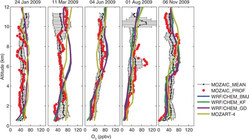
Fig. 10 MOZAIC observed and WRF-Chem simulated wind speed profiles are plotted corresponding to anomalous CO and O₃ profiles.

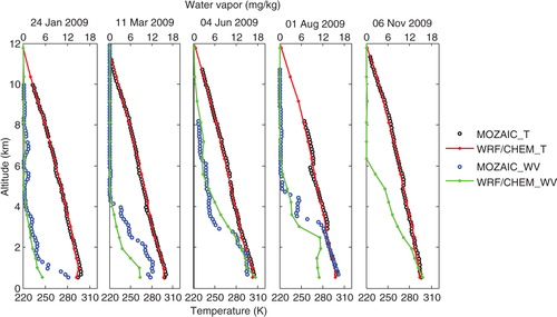
Fig. 11 Wind direction corresponding to anomalous CO and O₃ profiles obtained from MOZAIC observation and WRF-Chem simulations are plotted against altitude.

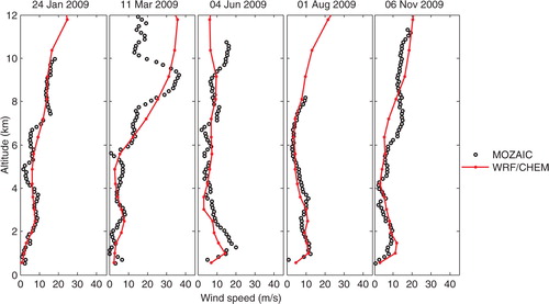
Fig. 12 WRF-Chem winds are plotted overlaid on O₃ (ppbv) at 2, 6 and 8 km altitude region at 6, 12 and 18 GMT. The O₃ over Hyderabad lies inside the box in the figure.

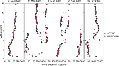
Fig. 13 WRF-Chem winds are plotted overlaid on CO (ppbv) at 2, 6 and 8 km altitude regions at 6, 12 and 18 GMT. The CO over Hyderabad lies inside the box in the figure.

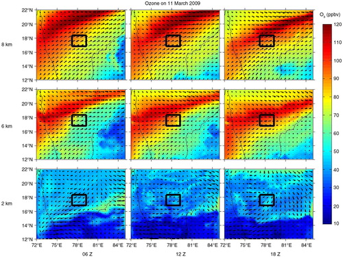
Table 5. Mean bias is calculated for WRF-Chem with respect to MOZAIC observations for temperature, water vapour mixing ratio and wind speed at different altitude region

Mean bias
Temperature (K)
Date	0–2 km	2–4 km	4–6 km	6–8 km	8–10 km
24 Jan 2009	1.9	−0.7	−0.6	0.3	−0.2
11 March 2009	0.4	0.0	−1.2	−0.2	0.6
4 June 2009	0.5	0.6	0.5	1.5	0.0
1 Aug 2009	0.5	1.2	−0.9	2.0	0.4
6 Nov 2009	1.4	−0.7	−0.1	−0.1	1.6
Water vapour mixing ratio (mg/kg)
24 Jan 2009	2.8	0.8	0.5	0.0	0.0
11 March 2009	4.6	3.0	0.1	0.0	0.0
4 June 2009	3.0	3.1	0.1	0.1	0.1
1 Aug 2009	0.1	−2.0	−0.4	−0.5	−0.3
Wind speed (m/s)
24 Jan 2009	0.6	1.1	−2.3	−1.9	0.4
11 March 2009	−1.6	−0.5	0.8	−2.3	1.5
4 June 2009	3.2	2.7	−1.6	0.3	−1.4
1 Aug 2009	0.2	0.0	0.9	0.3	0.8
6 Nov 2009	−2.0	−1.4	0.8	6.7	−0.4

In the monsoon profile (1 August 2009), there is uncertainty in wind direction (Fig. 11) between 5 and 7 km altitude region as well as an inversion in temperature in the MOZAIC temperature profile (Fig. 9) at the level of mid-troposphere (~6–7 km) which breaks at the altitude of ~7 km. The inversion in the temperature causes the high mixing of O₃ in MOZAIC profile at this altitude region (Fig. 8). However, the temperature inversion feature is completely missing in the WRF-Chem temperature profile and hence in the corresponding O₃ profile.

Fig. 8 The monthly mean MOZAIC O₃ profiles (MOZAIC_MEAN) for 5 months of the year 2009 are shown along with the standard deviation. The anomalous profile observed by MOZAIC for a particular month is shown along with the spatially and temporarily collocated profile simulated by WRF-Chem using BMJ, KF and GD convection schemes and MOZART-4 model.

The emission inventories have several sectors contributing to the emissions, but there are some sectors not included in one or two inventories. Due to these differences, the total emissions and associated uncertainties for the region are variable. In the present study, a simple grid-mapping program, ‘prep-chem-sources’ is used in the WRF-Chem model for global emission data. The ‘prep-chem-sources’ is an emission data generator package to provide gridded emission fluxes (kg/m²). We have used RETRO and EDGAR global inventories to generate the anthropogenic emission fluxes, whereas the biogenic emissions of trace species are calculated using MEGAN. Schultz et al. (2007) report several uncertainties associated with the RETRO emissions. These uncertainties include omission of specific sectors (e.g., railway traffic or cement manufacturing), underestimation of CO combustion emissions and NO_x ship traffic emissions, and the lack of weekly and diurnal profiles of emissions. For the Southeast Asia region, the RETRO seasonal cycle is based on the long-term O₃ Simulation and European Operational Smog (LOTOS-EUROS). Kurokawa et al. (2013) has shown that there is very little seasonal cycle for anthropogenic emissions of NO_x and black carbon over India, which is a region similar to Southeast Asia in terms of climate. Similarly for EDGAR, based on the detailed accounting of the emission control measures that have been put into operation after 1990, Cofala et al. (2007) identify large discrepancies in the transport sectors. EDGAR tends to estimate higher emissions from industry and the domestic sector, and lower emissions from transport, especially from non-road sources. In the MEGAN emissions, soil NO_x emissions are estimated to be uncertain, and these uncertainties could add to model-observation discrepancies during summer where heavy precipitation events are shown to induce strong pulses of NO_x (Ghude et al., 2010). Lightning NO_x emissions were not included in the simulations but are suggested to contribute very little to NO_x emissions over the Indian region (Ghude et al., 2010).

We analysed the CO and O₃ vertical profiles with WRF-Chem and MOZART-4 models which include both monthly averaged and anomalous profiles by taking MOZAIC observations as a reference. It has been found that both the models have reproduced CO and O₃ profiles within acceptable limits. We found the advantage with the simulations made by WRF-Chem over MOZART-4 in terms of meteorology that is coupled with chemistry in WRF-Chem model. We explain the two anomalous profiles (11 March and 1 August 2009) with the help of their meteorological parameters corresponding to them, which are simulated from WRF-Chem model.

This study is also a prototype of the simulations made using different convection schemes of WRF-Chem. It has been shown that a particular convection scheme can reproduce CO or O₃ profile better compared to other convection schemes. For example, in 24 January 2009 anomalous profile (Figs. 7 and 8), WRF-Chem reproduces CO and O₃ better by ~15 and 6 ppbv, respectively, with GD convection scheme in the near-surface tropospheric layer (0–2 km) compared to other convection schemes. It may be said that if we have prior determined conditions that qualify one of the convection schemes, it will result in a better simulation of chemical species.

8. Conclusion

The tropospheric CO and O₃ variability based on the MOZAIC and TES observations as well as WRF-Chem and MOZART-4 simulations have been studied in Hyderabad, India. The seasonal variability corresponding four different seasons have been discussed based on MOZAIC observations and TES retrieval. It is noted that the vertical profiles of O₃ retrieved from TES observations have less mean bias and standard deviation compared to CO profiles. It is also noted that TES retrieval of O₃ in autumn (SON) season is better compared to the other seasons with respect to MOZAIC observations. The time-dependent changes from MOZAIC and TES observations are analysed by taking differences of the smoothed monthly anomaly of CO and O₃. Table 2 summarises the interannual changes in the different regions of the troposphere. The near-surface (0–2 km) tropospheric CO and O₃ over Hyderabad shows a very significant increase from 2006 to 2010 with the MOZAIC observations. In 2–8 km tropospheric layer, both MOZAIC and TES have shown a very small decrease in CO; however, no significant interannual decrease is observed in O₃ in the same tropospheric layer from both the observations. In the 8–10 km tropospheric layer, MOZAIC observations have not shown any significant decrease in CO; however, very small decrease is found in O₃.

The WRF-Chem model simulates the meteorological variables as well as the chemical species. Therefore, the dynamics associated with CO and O₃ variability is also discussed using the meteorological parameters such as temperature, water vapour mixing ratio, wind speed and wind direction. Further, the CO and O₃ profiles have been reproduced using different convection schemes available within the WRF-Chem simulation. It has been found that the accuracy of different convection schemes differs in different regions of the troposphere.

The present work attempted to study the anomalous profiles of CO and O₃ obtained from the in situ observations of MOZAIC during 2009 using different convection schemes available in the WRF-Chem model. This study can also be extended using a different PBL scheme available within the WRF-Chem model since different PBL schemes present different kinds of mixing in the PBL which will impact the simulations further.

9. Acknowledgements

The authors acknowledge the strong support of the European Commission, Airbus and the Airlines (Lufthansa, Air-France, Austrian, Air Namibia, Cathay Pacific, Iberia and China Airlines so far) who carry the MOZAIC or IAGOS equipment and perform the maintenance since 1994. In its last 10 years of operation, MOZAIC has been funded by INSU-CNRS (France), Météo-France, Université Paul Sabatier (Toulouse, France) and Research Center Jëlich (FZJ, Jëlich, Germany). IAGOS has been additionally funded by the EU projects IAGOS-DS and IAGOS-ERI. The MOZAIC-IAGOS database is supported by ETHER (CNES and INSU-CNRS), now renamed as AERIS. The authors acknowledge the HPC facility of Physical Research Laboratory for running the model.

References

- Arakawa A. , Schubert W. H . Interaction of a cumulus cloud ensemble with the large-scale environment, Part I. J. Atmos. Sci. 1974; 31: 674–701. DOI: http://dx.doi.org/10.1175/1520–0469 .
- Beig G. , Brasseur G. P . Influence of anthropogenic emissions on tropospheric ozone and its precursors over the Indian tropical region during a monsoon. Geophys. Res. Lett. 2006; 33: L07808. DOI: http://dx.doi.org/10.1029/2005GL024949 .
- Betts A. K. , Miller M. J . A new convective adjustment scheme. Part II: single column tests using GATE wave, BOMEX, ATEX and arctic air-mass data sets. Q. J. Roy. Meteorol. Soc. 1986; 112(473): 693–709. DOI: http://dx.doi.org/10.1002/qj.49711247308 .
- Brasseur G. P. , Hauglustaine D. A. , Walters S. , Rasch P. J. , Müller J.-F. , co-authors . MOZART, a global chemical transport model for ozone and related chemical tracers: 1. Model description. J. Geophys. Res. Atmos. 1998; 103(D21): 28265–28289. DOI: http://dx.doi.org/10.1029/98JD02397 .
- Chen F. , Dudhia J . Coupling an advanced land-surface/hydrology model with the Penn State/NCAR MM5 modeling system, part I: model description and implementation. Mon. Weather Rev. 2001; 129: 569–585. DOI: http://dx.doi.org/10.1175/1520–0493 .
- Chou M.-D. , Suarez M. J. , Ho C.-H. , Yan M. M.-H. , Lee K.-T . Parameterizations for cloud overlapping and shortwave single-scattering properties for use in general circulation and cloud ensemble models. J. Clim. 1998; 11: 202–214. DOI: http://dx.doi.org/10.1175/1520–0442(1998) .
- Cofala J. , Amann M. , Klimont Z. , Kupiainen K. , Höglund-Isaksson L . Scenarios of global anthropogenic emissions of air pollutants and methane until 2030. Atmos. Environ. 2007; 41(38): 8486–8499. DOI: http://dx.doi.org/10.1016/j.atmosenv.2007.07.010 .
- Cooper O. R. , Parrish D.D. , Stohl A. , Trainer M. , Nédélec P. , co-authors . Increasing springtime ozone mixing ratios in the free troposphere over western North America. Nature. 2010; 463: 344–348. DOI: http://dx.doi.org/10.1038/nature08708 .
- Duncan B. N. , Logan J. A. , Bey I. , Megretskaia I. A. , Yantosca R. M. , co-authors . Global budget of co, 1988–1997: source estimates and validation with a global model. J. Geophys. Res. Atmos. 2007; 112: D22301. DOI: http://dx.doi.org/10.1029/2007JD008459 .
- Emmons L. K. , Hauglustaine D. A. , Müller J-F. , Carroll M. A. , Brasseur G. P. , co-authors . Data composites of airborne observations of tropospheric ozone and its precursors. J. Geophys. Res. 2000; 105: 20497–20538.
- Emmons L. K. , Walters S. , Hess P.G. , Lamarque J-F. , Pfister G.G. , co-authors . Description and evaluation of the Model for Ozone and Related chemical Tracers, version 4 (MOZART-4). Geosci. Model Dev. 2010; 3: 43–67. DOI: http://dx.doi.org/10.5194/gmd–3–43–2010 .
- Fishman J. , Solomon S. , Crutzen P. J . Observational and theoretical evidence in support of a significant in situ photochemical source of tropospheric ozone. Tellus. 1979; 31: 432–446.
- Gauss M. , Myhre G. , Pitari G. , Prather M. J. , Isaksen I. S. A. , co-authors . Radiative forcing in the 21st century due to ozone changes in the troposphere and the lower stratosphere. J. Geophys. Res Atmos. 2003; 108: D9. DOI: http://dx.doi.org/10.1029/2002JD002624 .
- Ghude S. D. , Lal D. M. , Beig G. , van der A., R. , Sable D . Rain-induced soil NOx emission from India during the onset of the summer monsoon: a satellite perspective. J. Geophys. Res. Atmos. 2010; 115: D16304. DOI: http://dx.doi.org/10.1029/2009JD013367 .
- Ghude S. D. , Pfister G. G. , Jena C. , van der A., R. J. , Emmons L. K. , co-authors . Satellite constraints of nitrogen oxide (NOx) emissions from India based on OMI observations and WRF-Chem simulations. Geophys. Res. Lett. 2013; 40: 1–6. DOI: http://dx.doi.org/10.1029/2012GL053926 .
- Girach I. , Nair P. R . Carbon monoxide over Indian region as observed by MOPITT. Atmos. Environ. 2014; 99: 599–609.
- Granier C. , Bessagnet B. , Bond T. , D'Angiola A. , Denier van der Gon H. , co-authors . Evolution of anthropogenic and biomass burning emissions of air pollutants at global and regional scales during the 1980–2010 period. Clim. Change. 2011; 9(1): 163–190.
- Grell G. A. , Dévényi D . A generalized approach to parameterizing convection combining ensemble and data assimilation techniques. Geophys. Res. Lett. 2002; 29(14): 38–1–38–4. DOI: http://dx.doi.org/10.1029/2002GL015311 .
- Guenther A. , Karl T. , Harley P. , Wiedinmyer C. , Palmer P. I. , Geron C . Estimates of global terrestrial isoprene emissions using MEGAN (Model of Emissions of Gases and Aerosols from Nature). Atmos. Chem. Phys. 2006; 6: 3181–3210. DOI: http://dx.doi.org/10.5194/acp–6–3181–2006 .
- Gummeneni S. , Yusup Y. B. , Chavali M. , Samadi S. Z . Source apportionment of particulate matter in the ambient air of Hyderabad city, India. Atmos. Res. 2011; 101: 752–754.
- Gurjar B. R. , van Aardenne J. A. , Lelieveld J. , Mohan M . Emission estimates and trends (1990–2000) for megacity Delhi and implications. Atmos. Environ. 2004; 38(33): 5663–5681. DOI: http://dx.doi.org/10.1016/j.atmosenv.2004.05.057 .
- Hack J. J. , Boville B. A. , Kiehl J. T. , Rasch P. J. , Williamson D. L . Climate statistics from the National Center for Atmospheric Research Community Climate Model CCM2. J. Geophys. Res. Atmos. 1994; 99: 20785–20813. DOI: http://dx.doi.org/10.1029/94JD01570 .
- Holloway T. , Levy I. H. , Kasibhatla P . Global distribution of carbon monoxide. J. Geophys. Res. 2000; 105: 12123–12112.
- Holstlag A. , Boville B. A . Local versus nonlocal boundary-layer diffusion in a global climate model. J. Clim. 1993; 6: 1825–1842.
- Horowitz L. W. , Walters S. , Mauzerall D. L. , Emmons L. K. , Rasch P. J. , co-authors . A global simulation of tropospheric ozone and related tracers: description and evaluation of MOZART, version 2. J. Geophys. Res. Atmos. 2003; 108: 4784. DOI: http://dx.doi.org/10.1029/2002JD002853 .
- Hu X.-M. , Nielsen-Gammon J. W. , Zhang F. Q . Evaluation of three planetary boundary layer schemes in the WRF model. J. Appl. Meteorol. Climatol. 2010; 49(9): 1831–1844. DOI: http://dx.doi.org/10.1175/2010jamc2432.1 .
- Janjić Z. I . The step-mountain coordinate: physical package. Mon. Weather Rev. 1990; 118: 1429–1443. DOI: http://dx.doi.org/10.1175/1520–0493(1990) .
- Kain J. S . The Kain–Fritsch convective parameterization: an update. J. Appl. Meteorol. 2004; 43: 170–181.
- Kain J. S. , Fritsch J. M . A one-dimensional entraining/detraining plume model and its application in convective parameterization. J. Atmos. Sci. 1990; 47: 2784–2802.
- Khalil M. A. K. , Rasmussen R. A . Global decrease in atmospheric carbon monoxide. Nature. 1994; 370: 639–641.
- Kulkarni P. S. , Ghude S. D. , Bortoli D . Tropospheric ozone (TOR) trend over three major inland Indian cities: Delhi, Hyderabad and Bangalore. Ann. Geophys. 2010; 28(10): 1879–1885. DOI: http://dx.doi.org/10.5194/angeo-28-1879-2010 .
- Kurokawa J. , Ohara T. , Morikawa T. , Hanayama S. , Janssens-Maenhout G. , co-authors . Emissions of air pollutants and greenhouse gases over Asian regions during 2000–2008: regional emission inventory in ASia (REAS) version 2. Atmos. Chem. Phys. 2013; 13(21): 11019–11058. DOI: http://dx.doi.org/10.5194/acp-13-11019-2013 .
- Lamarque J.-F. , Bond T.C. , Eyring V. , Granier C. , Heil A. , co-authors . Historical (1850–2000) gridded anthropogenic and biomass burning emissions of reactive gases and aerosols: methodology and application. Atmos. Chem. Phys. 2010; 10(15): 7017–7039. DOI: http://dx.doi.org/10.5194/acp-10-7017-2010 .
- Law K . More ozone over North America. Nature. 2010; 463: 307–308.
- Lin S. J. , Rood R. B . Multidimensional flux-form semi-Lagrangian transport scheme. Mon. Weather Rev. 1996; 124: 2046–2070.
- Lopez J. P. , Luo M. , Christensen L. E. , Loewenstein M. , Jost H. , co-authors . TES carbon monoxide validation during two AVE campaigns using the ARGUS and ALIAS instruments on NASA's WB-57F. J. Geophys. Res. 2008; 113: D16S47. DOI: http://dx.doi.org/10.1029/2007JD008811 .
- Luo M. , Rinsland C. P. , Rodgers C. D. , Logan J. A. , Worden H. , co-authors . TES carbon monoxide validation with DACOM aircraft measurements during INTEX-B 2006. J. Geophys. Res. 2007a; 112: D24S48. DOI: http://dx.doi.org/10.1029/2007JD008803 .
- Luo M. , Rinsland C. P. , Rodgers C. D. , Logan J. A. , Worden H. , co-authors . Comparison of carbon monoxide measurements by TES and MOPITT: influence of a priori data and instrument characteristics on nadir atmospheric species retrievals. J. Geophys. Res. 2007b; 112: D09303. DOI: http://dx.doi.org/10.1029/2006JD007663 .
- Marenco A. , Thouret V. , Nédélec P. , Smit H. , Helten M. , co-authors . Measurement of ozone and water vapour by airbus in-service aircraft: the MOZAIC airborne program, an overview. J. Geophys. Res. Atmos. 1998; 103: 25631–25642. DOI: http://dx.doi.org/10.1029/98JD00977 .
- Mlawer E. J. , Taubaman S. J. , Brown P. D. , Iacono M. J. , Clough S. A . Radiative transfer for inhomogeneous atmosphere: RRTM, a validated correlated-k model for the longwave. J. Geophys. Res. 1997; 102(D14): 16663–16682. DOI: http://dx.doi.org/10.1029/97JD00237 .
- Monks P. S. , Granier C. , Fuzzi S. , Stohl A. , Williams M. L. , co-authors . Atmospheric composition change – global and regional air quality. Atmos. Environ. 2009; 43(33): 5268–5350.
- Nakanishi M. , Niino H . An improved Mellor-Yamada Level-3 model: its numerical stability and application to a regional prediction of advection fog, boundary layer meteorology. Atmos. Environ. 2006; 119: 397–407. DOI: http://dx.doi.org/10.1007/s10546–005–9030–8 .
- Ohara T. , Akimoto H. , Kurokawa J. , Horii N. , Yamaji K. , co-authors . An Asian emission inventory of anthropogenic emission sources for the period 1980–2020. Atmos. Chem. Phys. Discuss. 2007; 7: 6843–6902. DOI: http://dx.doi.org/10.5194/acpd–7–6843–2007 .
- Petropavlovskikh I. , Ahn C. , Bhartia P. K. , Flynn L. E . Comparison and covalidation of ozone anomalies and variability observed in SBUV(/2) and Umkehr Northern midlatitude ozone profile estimates. Geophys. Res. Lett. 2005; 32: L06805. DOI: http://dx.doi.org/10.1029/2004GL022002 .
- Piegorsch W. W . Tables of P-values for T-and Chi-Square Reference Distributions. 2002; Technical Report no. 194. Department of Statistics, University of South Carolina, Columbia, SC.
- Prasad A. K. , Singh R. P. , Kafatos M . Influence of coal based thermal power plants on aerosol optical properties in the Indo-Gangetic basin. Geophys. Res. Lett. 2006; 33: L05805. DOI: http://dx.doi.org/10.1029/2005GL023801 .
- Prasad A. K. , Singh R. P. , Kafatos M . Influence of coal-based thermal power plants on the spatial-temporal variability of tropospheric NO2 column over India. Environ. Monit. Assess. 2011; 184: 1891–1907.
- Sahu L. K . Volatile organic compounds and their measurements in the troposphere. Curr. Sci. 2012; 102(10): 1645–1649.
- Sahu L. K. , Sheel V. , Kajino M. , Gunthe S. S. , Thouret V. , co-authors . Characteristics of tropospheric ozone variability over an urban site in Southeast Asia: a study based on MOZAIC and MOZART vertical profiles. J. Geophys. Res. Atmos. 2013; 118(15): 8729–8747. DOI: http://dx.doi.org/10.1002/jgrd.50662 .
- Sahu S. K. , Beig G. , Parkhi N . Critical emissions from the largest on-road transport network in South Asia. Aerosol Air Qual. Res. 2014; 14: 135–144.
- Sauvage B. , Martin R. V. , van Donkelaar A. , Ziemke J. R . Quantification of the factors controlling tropical tropospheric ozone and the south Atlantic maximum. J. Geophys. Res. 2007b; 112: 11309.
- Schell B. , Ackermann I. J. , Hass H. , Binkowski F. S. , Ebel A . Modeling the formation of secondary organic aerosol within a comprehensive air quality model system. J. Geophys. Res. 2001; 106: 28275–28293. DOI: http://dx.doi.org/10.1029/2001JD000384 .
- Schultz M. , Rast S. , van het Bolscher M. , Pulles T. , Pereira J. , co-authors . Reanalysis of the Tropospheric Chemical Composition Over the Past 40 Years, a Long-Term Global Modeling Study of Tropospheric Chemistry Funded Under the 5th EU Framework Programme. 2007. Technical Report, EU-Contract No. EVK2-CT-2002-00170, 184. Online at: http://retro.enes.org/reports/D1–6_final.pdf .
- Seinfeld J. H. , Pandis S. N . From Air Pollution to Climate Change, Atmospheric Chemistry and Physics. 2006; New York. Atmospheric Chemistry and Physics: Wiley.
- Sheel V. , Sahu L. K. , Kajino M. , Deushi M. , Stein O. , Nedelec P . Seasonal and interannual variability of carbon monoxide based on MOZAIC observations, MACC reanalysis, and model simulations over an urban site in India. J. Geophys. Res. Atmos. 2014; 119: 9123–9141. DOI: http://dx.doi.org/10.1002/2013JD021425 .
- Srivastava S. , Sheel V . Study of tropospheric CO and O3 enhancement episode over Indonesia during autumn 2006 using the Model for Ozone and Related chemical Tracers (MOZART-4). Atmos. Environ. 2013; 67: 53–62. DOI: http://dx.doi.org/10.1016/j.atmosenv.2012.09.067 .
- Stockwell W. R. , Middleton P. , Chang J. S. , Tang X . The second generation regional acid deposition model chemical mechanism for regional air quality modeling. J. Geophys. Res. 1990; 95: 16343–16367. DOI: http://dx.doi.org/10.1029/JD095iD10p16343 .
- Thouret V. , Marenco A. , Logan J. A. , Nédélec P. , Grouhel C . Comparisons of ozone measurements from the MOZAIC airborne program and the ozone sounding network at eight locations. J. Geophys. Res. 1998b; 103: 25695–25720.
- Thouret V. , Marenco A. , Nédélec P. , Grouhel C . Ozone climatologies at 9–12 km altitude as seen by the MOZAIC airborne program between September 1994 and August 1996. J. Geophys. Res. 1998a; 103: 25653–25680.
- van Vuuren D. P. , Edmonds J. , Kainuma M. , Riahi K. , Thomson A. , co-authors . The representative concentration pathways: an overview. Clim. Change. 2011; 109(1–2): 5–31. DOI: http://dx.doi.org/10.1007/s10584-011-0148-z .
- Venkataraman C. , Habib G. , Kadamba D. , Shrivastava M. , Leon J.-F. , co-authors . Emissions from open biomass burning in India: Integrating the inventory approach with high-resolution Moderate Resolution Imaging Spectroradiometer (MODIS) active-fire and land cover data. Global Biogeochem. Cycles. 2006; 20: GB2013. DOI: http://dx.doi.org/10.1029/2005GB002547 .
- Wang Y. , Jacob D. J. , Logan J. A . Global simulation of tropospheric O3–NOx–hydrocarbon chemistry: 3. Origin of tropospheric ozone and effects of nonmethane hydrocarbons. J. Geophys. Res. Atmos. 1998; 103: 10757–10767. DOI: http://dx.doi.org/10.1029/98JD00156 .
- Wiedinmyer C. , Akagi S. K. , Yokelson R. J. , Emmons L. K. , Al-Saadi J. A. , co-authors . The Fire INventory from NCAR (FINN): a high resolution global model to estimate the emissions from open burning. Geosci. Model Dev. 2011; 4(3): 625–641. DOI: http://dx.doi.org/10.5194/gmd–4–625–2011 .
- Wigley T. M. L. , Smith S. J. , Prather M. J . Radiative forcing due to reactive gas emissions. J. Clim. 2002; 15: 2690–2696.
- Worden H. M. , Deeter M. N. , Frankenberg C. , George M. , Nichitiu F. , co-authors . Decadal record of satellite carbon monoxide observations. Atmos. Chem. Phys. 2013; 13: 837–850. DOI: http://dx.doi.org/10.5194/acp–13–837–2013 .
- Worden J. , Kulawik S. S. , Shephard M. W. , Clough S. A. , Worden H. , co-authors . Predicted errors of tropospheric emission spectrometer nadir retrievals from spectral window selection. J. Geophys. Res. Atmos. 2004; 109(D9): D09308, DOI: http://dx.doi.org/10.1029/2004JD004522 .
- Zhang G. J. , MacFarlane N. A . Sensitivity of climate simulations to the parameterization of cumulus convection in the Canadian climate centre general circulation model. Atmos. Ocean. 1995; 33: 407–446.
- Zhang L. , Jacob D. J. , Liu X. , Logan J. A. , Chance K. , co-authors . Intercomparison methods for satellite measurements of atmospheric composition: application to tropospheric ozone from TES and OMI. Atmos. Chem. Phys. 2010; 10: 4725–4739. DOI: http://dx.doi.org/10.5194/acp–4710–4725–2010 .