The False Positive Risk: A Proposal Concerning What to Do About p-Values

Figures & data

Fig. 1 Plot of FPR against normalized effect size, with power kept constant throughout the curves by varying n. The dashed blue line shows the FPR calculated by the p-less-than method. The solid blue line shows the FPR calculated by the p-equals method. This example is calculated for an observed p-value of 0.05, with power kept constant at 0.78 (power calculated conventionally at p = 0.05), with prior probability P(H₁) = 0.5. The sample size needed to keep the power constant at 0.78 varies from n = 1495 at effect size = 0.1, to n = 5 at effect size = 2.0 (the range of plotted values). The dotted red line marks an FPR of 0.05, the same as the observed p-value. Calculated with Plot-FPR-v-ES-constant-power.R, output file: FPR-vs-ES-const-power.txt (supplementary material).

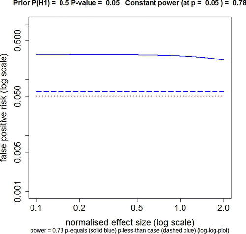
Fig. 2 FPR plotted against n, the number of observations per group for a two independent sample t-test, with normalized true effect size of 1 standard deviation. The FPR is calculated by the p-equals method, with a prior probability P(H₁) = 0.5 (Equation A6(A6) $$\text{FPR}=\frac{1}{1+L_{10}\frac{P\left({\mathrm{H}}_1\right)}{1-P\left({\mathrm{H}}_1\right)}}$$(A6) ). Log–log plot. Calculations for four different observed p-values, from top to bottom these are: p = 0.05 (blue), p = 0.01 (green), p = 0.001 (red), p = 0.0001 (orange). The power of the tests varies throughout the curves. For example, for the p = 0.05 curve, the power is 0.22 for n = 4 and power is 0.9999 for n = 64 (the extremes of the plotted range). The minimum FPR (marked with gray-dashed lines) is 0.206 at n = 8. This may be compared with the FPR of 0.27 at n = 16, at which point the power is 0.78 (as in Colquhoun, (2014), (2017)). Values for other curves are given in the print file for these plots (Calculated with Plot-FPR-vs-n.R. Output file: Plot-FPR-vs-n.txt. supplementary material).

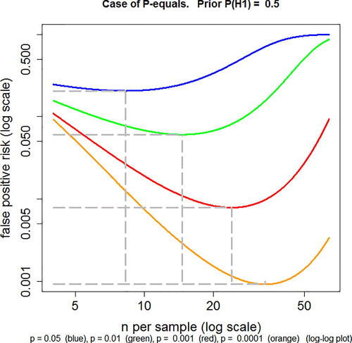
Table 1 Calculations done with web calculator http://fpr-calc.ucl.ac.uk/, or with R scripts (see the appendix).

			Minimum FPR (mFPR)			False positive risk, FPR with
			prior = 0.5			prior = 0.1
Observed	Likelihood	Prior for	Colquhoun	Sellke–Berger	Goodman	Colquhoun	Sellke–Berger	Goodman
p-value	ratio: (H1/H0)	FPR = 0.05	value	value	value	value	value	value
0.05	2.8	0.87	0.27	0.29	0.227	0.76	0.79	0.725
0.025	6.1	0.76	0.14	0.20	0.140	0.60	0.69	0.593
0.01	15	0.55	0.061	0.11	0.068	0.37	0.53	0.395
0.005	29	0.40	0.034	0.067	0.037	0.24	0.39	0.259
0.001	100	0.16	0.0099	0.018	0.0088	0.082	0.14	0.074

NOTES: Column 1: The observed p-value.

Column 2: Likelihood ratios (likelihood for there being a real effect divided by likelihood of null hypothesis). Calculated for a well-powered (0.78) experiment, as in Equation (A5)(A5) $$L_{10}=\frac{L\left({\mathrm{H}}_1\right)}{L\left({\mathrm{H}}_0\right)}=\frac{\text{Prob}\left(\text{data}\right|H_1)}{\text{Prob}\left(\text{data}\right|H_0)}=\frac{y_1}{2y_0}$$(A5) and Colquhoun (2017).

Column 3: The prior probability of there being a real effect, P(H₁), that it would be necessary to postulate in order to achieve an FPR (FPR) of 5%. Calculated for a well-powered (0.78) experiment as in Equation (A7)(A7) $$P\left({\mathrm{H}}_1\right)=\frac{(1-\text{FPR})}{(1-\text{FPR}+L_{10}\text{FPR})}$$(A7) . (The reverse Bayes approach: Colquhoun (2017)).

Columns 4–6: The minimum FPR, that is, the FPR that corresponds to prior probability of P(H₁) = 0.5, calculated by three methods, Colquhoun value (calculated for a well-powered (0.78) experiment as in Equations (A5)(A5) $$L_{10}=\frac{L\left({\mathrm{H}}_1\right)}{L\left({\mathrm{H}}_0\right)}=\frac{\text{Prob}\left(\text{data}\right|H_1)}{\text{Prob}\left(\text{data}\right|H_0)}=\frac{y_1}{2y_0}$$(A5) and (A6)(A6) $$\text{FPR}=\frac{1}{1+L_{10}\frac{P\left({\mathrm{H}}_1\right)}{1-P\left({\mathrm{H}}_1\right)}}$$(A6) and Colquhoun (2017). Sellke–Berger value: calculated as in Equations (A8)(A8) $$L_{10}=\frac{1}{-\mathit{ep}\hspace{0.17em}\text{log}\hspace{0.17em}\left(p\right)}$$(A8) and (A6)(A6) $$\text{FPR}=\frac{1}{1+L_{10}\frac{P\left({\mathrm{H}}_1\right)}{1-P\left({\mathrm{H}}_1\right)}}$$(A6) . Goodman value, calculated as in Equations (A9)(A9) $$L_{10}=\frac{1}{2\hspace{0.17em}\text{exp}\hspace{0.17em}(-z^2/2)}$$(A9) and (A6)(A6) $$\text{FPR}=\frac{1}{1+L_{10}\frac{P\left({\mathrm{H}}_1\right)}{1-P\left({\mathrm{H}}_1\right)}}$$(A6) .

Columns 7–9. As columns 4–6, but for an implausible hypothesis with prior probability, P(H₁) = 0.1.

Fig. 3 Comparison of three approaches to calculation of FPR in the case of a simple alternative hypothesis. Solid blue line: the p-equals method for t-tests described in Colquhoun (2017), and Equations (A5)(A5) $$L_{10}=\frac{L\left({\mathrm{H}}_1\right)}{L\left({\mathrm{H}}_0\right)}=\frac{\text{Prob}\left(\text{data}\right|H_1)}{\text{Prob}\left(\text{data}\right|H_0)}=\frac{y_1}{2y_0}$$(A5) and (A6)(A6) $$\text{FPR}=\frac{1}{1+L_{10}\frac{P\left({\mathrm{H}}_1\right)}{1-P\left({\mathrm{H}}_1\right)}}$$(A6) . Dashed blue line: the Sellke–Berger approach, using Equations (A8)(A8) $$L_{10}=\frac{1}{-\mathit{ep}\hspace{0.17em}\text{log}\hspace{0.17em}\left(p\right)}$$(A8) and (A6)(A6) $$\text{FPR}=\frac{1}{1+L_{10}\frac{P\left({\mathrm{H}}_1\right)}{1-P\left({\mathrm{H}}_1\right)}}$$(A6) . Dotted blue line: the Goodman approach, calculated using Equations (A9)(A9) $$L_{10}=\frac{1}{2\hspace{0.17em}\text{exp}\hspace{0.17em}(-z^2/2)}$$(A9) and (A6)(A6) $$\text{FPR}=\frac{1}{1+L_{10}\frac{P\left({\mathrm{H}}_1\right)}{1-P\left({\mathrm{H}}_1\right)}}$$(A6) . Dotted red line is where points would lie if FPR was equal to the p-value. This example is calculated for n = 16, normalized effect size = 1 and prior probability P(H₁) = 0.5. Log–log plot. Calculated with Plot-FPR-vs-Pval + Sellke-Goodman.R (supplementary material).

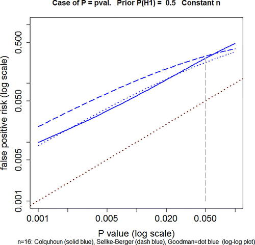
Table 2 Response in hours extra sleep (compared with controls) induced by (–)-hyoscyamine (A) and (–)-hyoscine (B). From Cushny and Peebles (1905).

Drug A yA	Drug B yB
+0.7	+1.9
−1.6	+0.8
−0.2	+1.1
−1.2	+0.1
−0.1	−0.1
+3.4	+4.4
+3.7	+5.5
−0.8	+1.6
0.0	+4.6
+2.0	+3.4

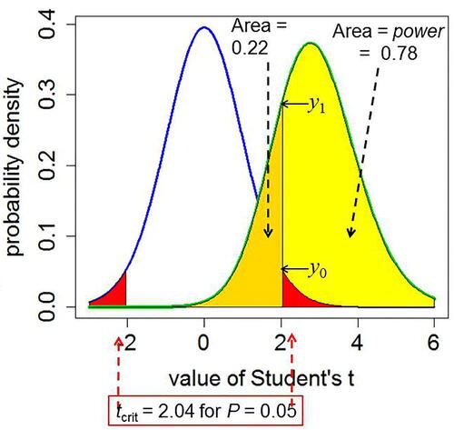
Fig. A1 Definitions for a null hypothesis significance test: reproduced from Colquhoun (2017). A Student’s t-test is used to analyze the difference between the means of two groups of n = 16 observations. The t value, therefore, has 2(n – 1) = 30 d.f. The blue line represents the distribution of Student’s t under the null hypothesis (H₀): the true difference between means is zero. The green line shows the noncentral distribution of Student’s t under the alternative hypothesis (H₁): the true difference between means is 1 (1 SD). The critical value of t for 30 d.f. and p = 0.05 is 2.04, so, for a two-sided test, any value of t above 2.04, or below –2.04, would be deemed “significant.” These values are represented by the red areas. When the alternative hypothesis is true (green line), the probability that the value of t is below the critical level (2.04) is 22% (gold shaded): these represent false negative results. Consequently, the area under the green curve above t = 2.04 (shaded yellow) is the probability that a “significant” result will be found when there is in fact a real effect (H₁ is true): this is the power of the test, in this case 78%. The ordinates marked y₀ (= 0.526) and $y_1(=0.290)$ are used to calculate likelihood ratios for the p-equals case.

Colquhoun, D. (2014), “An Investigation of the False Discovery Rate and the Misinterpretation of p-values,” Royal Society Open Science, 1, 140216, available http://rsos.royalsocietypublishing.org/content/1/3/140216

 PubMed Web of Science ®Google Scholar

Colquhoun, D. (2017), “The Reproducibility of Research and the Misinterpretation of P Values,” Royal Society Open Science, 4, 171085, available at http://rsos.royalsocietypublishing.org/content/4/12/171085.

 PubMed Web of Science ®Google Scholar

Cushny, A. R., & Peebles, A. R. (1905), “The Action of Optical Isomers: II. Hyoscines,” The Journal of Physiology, 32, 501–510, available at https://physoc.onlinelibrary.wiley.com/doi/abs/10.1113/jphysiol.1905.sp001097 DOI: 10.1113/jphysiol.1905.sp001097.

 PubMedGoogle Scholar