An Introduction to Second-Generation p-Values

Figures & data

Fig. 1 Illustration of a point null hypothesis, H₀; the estimated effect that is the best supported hypothesis, $\widehat{H}=\widehat{\theta }$; the confidence interval (CI) for the estimated effect [${\text{CI}}^{-},{\text{CI}}^{+}$]; and the interval null hypothesis $[H_0^{-},H_0^{+}]$.

Table 1 Comparison between the classical and second-generation p-value.

Property	Classical p-value	Second-generation p-value
Null hypothesis	Point	Interval
Scale	Number between 0 and 1, excluding zero	Number between 0 and 1, inclusive
Able to indicate support for alternative hypotheses	When small or near 0	When 0
Able to indicate data are inconclusive	When larger than the stated cutoff for significance	When between 0 and 1; near 1/2 is strictly inconclusive
Able to indicate support for null hypotheses	No	When 1
Accounts for practical importance	No	Yes, via specification of the null
Comparable across datasets	Yes, when the sample size is equal	Yes, when the width of the interval null is equal
Interpretation	Awkward, conditions on null hypothesis	Straightforward, conditions on observed data
Assumptions needed for computation	Probability model, sharp null hypothesis, sample space	Probability model, interval null hypothesis
Requires threshold for interpretation	Generally, yes	No, intended as a descriptive statistic
Adjustments required for multiple comparisons/looks?	Yes, if considered a Type I error rate; no, if considered a measure of statistical evidence	No

Fig. 2 Manhattan plot of SNP associations, colored according to second-generation p-value status. The x-axis shows SNP position on chromosome 6 and the position of the organic cation transporter gene (SLC22A3). The top 16 associations by p-value rank are in green and the top 16 associations by second-generation p-value rank are in black. Bonferroni, FDR, and unadjusted significance levels are show by dashed lines.

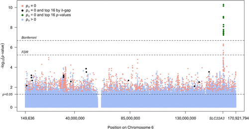
Fig. 3 Modified Manhattan-style plot of SNP associations as measured by the delta-gap. Points are colored according to second-generation p-value status. The x-axis shows SNP position on chromosome 6 and the position of the organic cation transporter gene (SLC22A3). The top 16 associations by p-value rank are in green and the top 16 associations by second-generation p-value rank are in black.

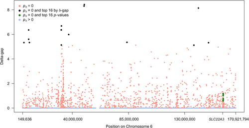
Fig. 4 1/8 likelihood SIs for the estimated odds ratio for SNPs with the smallest 500 p-values. The x-axis is p-value rank. The interval null hypothesis (in gray) ranges from 0.9 to 1.1111 (= 1/0.9). Intervals are colored according to second-generation p-value status. The top 16 Bonferroni SNPs are in green and the top 16 SGPV SNPs are in black. Bonferroni (“Bonf”) and FDR significance levels are shown by dashed lines.

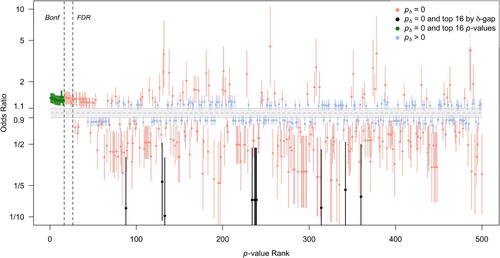
Fig. 5 Mirrored waterfall plot. 1/8 likelihood SIs for the estimated odds ratio for SNPs in the top 2,000 second-generation p-value ranking. The x-axis is SGPV rank. The interval null hypothesis (in gray) ranges from 0.9 to 1.1111 (= 1/0.9). Intervals are colored according to second-generation p-value status. The top 16 Bonferroni SNPs are in green and the top 16 SGPV SNPs are in black.

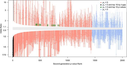
Fig. 6 Cross-tabulation of classical p-values and second-generation p-values in the prostate cancer data example.

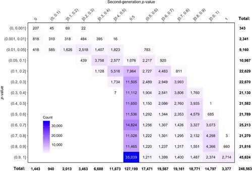
Table 2 False discovery rates of 5 SGPV = 0 findings computed under various null and alternative hypothesis configurations.

			Odds	1/8 SI	1/8 SI
SNP ID	SGPV rank	p-Value rank	ratio	lower limit	upper limit	FDR1	FDR2	FDR3
kgp4568244_C	1	133	0.10	0.03	0.37	2.9%	17.1%	3.3%
kgp8051290_G	13	2002	15.58	1.95	124.68	4.3%	30.3%	4.9%
kgp4497498_A	28	255	4.37	1.80	10.64	2.5%	8.6%	3.1%
rs3123636_G	423	1	1.39	1.26	1.55	0.004%	0.1%	0.4%
kgp7460928_G	1443	3310	1.78	1.11	2.87	2.4%	2.0%	3.0%

NOTE: The prior probability ratio, r, is set to 1.