The p-value Function and Statistical Inference

Figures & data

Fig. 1 The upper graph presents the model at some typical θ value and the observed data value $y^{\text{obs}}$; the lower graph records in addition the p-value and the likelihood for that θ value, and also in dots the density using the maximum likelihood $\theta ={\widehat{\theta }}^{\text{obs}}$ value for the parameter.

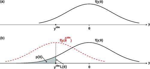
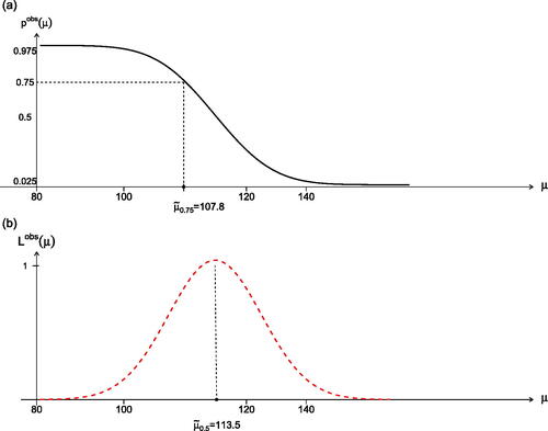
Fig. 2 The upper graph presents the p-value function and the lower graph the likelihood function, for the simple Normal example; the median estimate of θ is ${\widehat{\theta }}_{0.50}$ which here is the maximum likelihood value ${\widehat{\theta }}^{\text{obs}}=10$.

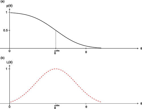
Fig. 3 The upper graph (a) indicates the median estimate and the one-sided 0.975 and 0.025 confidence bounds; the lower graph (b) records the observed likelihood function.

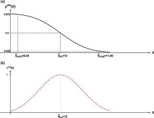
Fig. 4 The p-value function for n = 1 (solid), n = 4 (dashed), n = 100 (dotted).

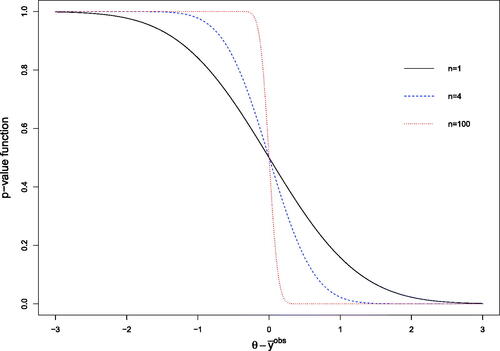
Fig. 5 The sample space for a sample of 2 from the uniform distribution on $(\theta -1/2,\theta +1/2)$. The observed data point is $(9.4,8.6)$; the square is the sample space for $\theta ={\widehat{\theta }}^{\text{obs}}={\overline{y}}^{\text{obs}}=9$. Only θ-values in the range 8.9–9.1 can put positive density at the observed data point. The short line through this point illustrates the small data range consistent with the observed data.

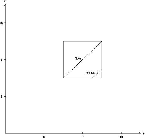
Fig. 6 The approximate density of $\overline{y}$ for some θ value.

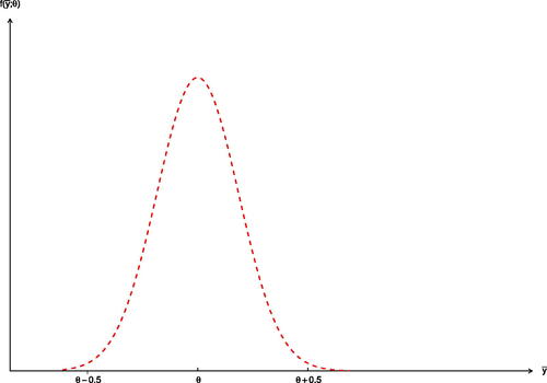
Fig. 7 The observed p-value function from the approximate pivot $t=({\overline{y}}^{\text{obs}}-\theta )/2^{-1/2}{(1/12)}^{1/2}=0.20({\overline{y}}^{\text{obs}}-\theta )$ as a function of θ.

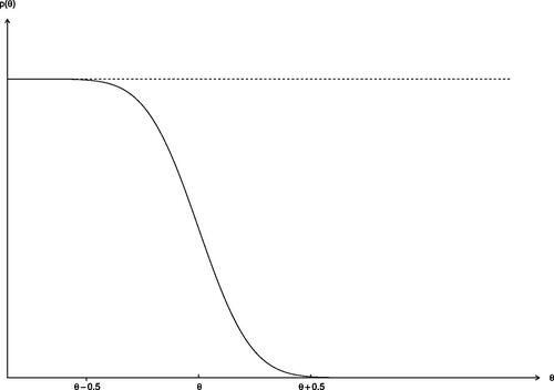
Fig. 8 The exact observed a likelihood function from the data $(9.4,8.6)$.

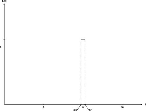
Fig. 9 For the simple exponential model, the p-value function is plotted using the Normal approximation for r (dotted), using the third-order approximation (dashed), and compared to the exact p-value function (solid).

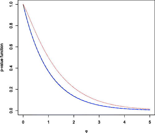
Fig. 10 A log-likelihood function with the log-likelihood ratio $r^2/2$ and the standardized maximum likelihood departure $q=(\phi -\widehat{\phi }){\mathcal{J}}_{\phi \phi }^{1/2}$ identified.

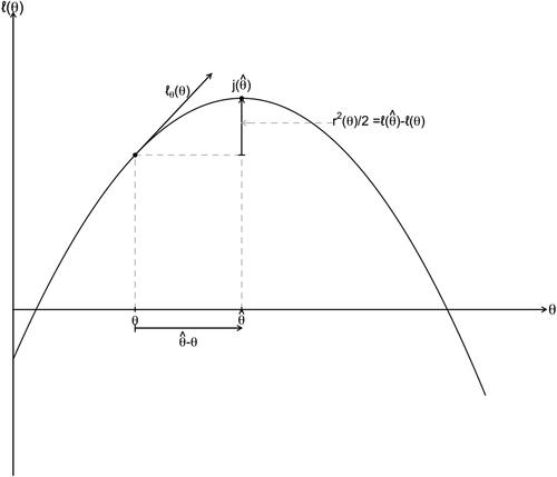
Fig. 11 The p-value function and log-likelihood function for the mean of the Gamma model data from Gross and Clark (1975).

Gross, A., and Clark, V. (1975), Survival Distributions: Reli-ability Applications in the Biomedical Sciences. New York: Wiley.

 Google Scholar