Discontinuous Galerkin isogeometric analysis for segmentations generating overlapping regions

Figures & data

Figure 1. (a) A conforming multipatch representation of Ω, (b) the inaccurate control points and the non-conforming multipatch representation of Ω.

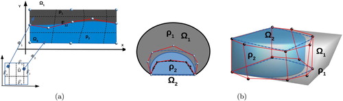
Figure 2. (a) Illustration of a patch representation with the overlapping region ${\mathrm{\Omega }}_{o21}$ in 2d and the diametrically opposite points on $\mathrm{\partial }{\mathrm{\Omega }}_{o21}$, (b) overlapping patches in 3d, (c) the images of the faces of $\mathrm{\partial }\hat{\mathrm{\Omega }}$ under the mappings ${\mathbf{\Phi }}_i^{\ast },i=1,2$ in 2d, (d) the images of the faces of $\mathrm{\partial }\hat{\mathrm{\Omega }}$ in 3d.

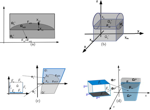
Figure 3. (a) Configuration of the faces and the edges on $\mathrm{\partial }{\mathrm{\Omega }}_{o12}$ and their corresponding edges on $\mathrm{\partial }\hat{\mathrm{\Omega }}$ which are used to compute the interface integrals, (b) an example of an overlapping region with more than two faces. The relative edges on the opposite faces must again match.

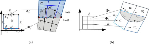
Table 1. The values of the expected rates r as they result from estimate (63(63) $\parallel u-u_h^{\ast }{\parallel }_{DG}\le \tilde{C}\left(h^s\sum _{i=1}^2(\parallel u{\parallel }_{H^{\ell }\left({\mathrm{\Omega }}_i^{\ast }\right)}+\parallel u_i^{\ast }{\parallel }_{H^{\ell }\left({\mathrm{\Omega }}_i^{\ast }\right)})+d_o\parallel f{\parallel }_{L^2\left(\mathrm{\Omega }\right)}+h^{\text{β}}({\mathcal{K}}_o\left(u\right)+{\mathcal{K}}_o\left(u^{\ast }\right))\right),$(63) ).

	B-spline degree p
	Smooth solutions, $u\in H^{\ell \ge p+1}$
$d_o=h^{\lambda }$	$\lambda =1$	$\lambda =2$	$\lambda =2.5$	$\lambda =3$
$\text{β}:=$	0.5	1.5	2	2.5
$s:=$	p	p	p	p
$r:=$	0.5	1.5	$min(p,\text{β})$	$min(p,\text{β})$

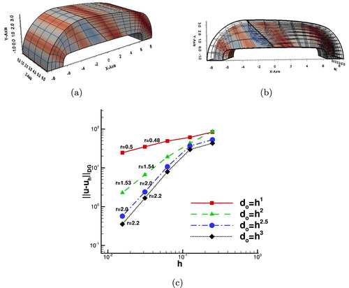
Figure 4. Example 4.1: (a) The patches ${\mathrm{\Omega }}_i^{\ast }$ with the initial non-matching meshes and the contours of the exact solution. (b) The contours of the $u_h^{\ast }$ solution for $d_o=h$. (c) The convergence rates for the different values of λ.

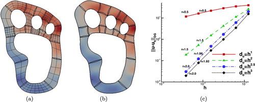
Figure 5. Example 4.2: (a) The overlapping patches ${\mathrm{\Omega }}_i^{\ast }$ and the pattern of diffusion coefficients ${\rho }_i$, (b) The contours of $u_h^{\ast }$ on every ${\mathrm{\Omega }}_i$ computed with $d_0=0.06$, (c) The convergence rates for the four choices of λ.

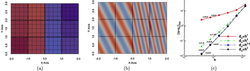
Figure 6. Example 4.3: (a) The overlapping patches ${\mathrm{\Omega }}_i^{\ast }$ and the multiple curve boundary of the overlapping region, (b) The contours of $u_h^{\ast }$ on every ${\mathrm{\Omega }}_i$ computed on the second mesh level, (c) The convergence rates for the four choices of λ.

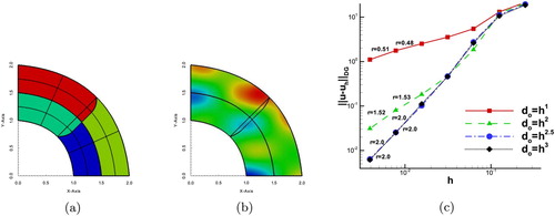
Figure 7. Example 4, $\mathrm{\Omega }\subset {\mathbb{R}}^3$: (a) The physical patches with an initial coarse mesh and the contours of the exact solution, (b) The contours of $u_h^{\ast }$ computed on ${\mathrm{\Omega }}_1^{\ast }\cup {\mathrm{\Omega }}_2^{\ast }$ with $d_o=1.5$, (c) Convergence rates r for the four values of λ.