Thermochemical oscillation of methane MILD combustion diluted with N₂/CO₂/H₂O

Figures & data

Table 1. Experiment initial conditions.

Cases	CH4	O2	N2	CO2	H2O
A	0.0333	0.0667	0.9	0.0	0.0
B	0.0333	0.0667	0.0	0.9	0.0
C	0.0333	0.0667	0.495	0.0	0.405

Table 2. Similar experimental data in JSR.

Case	Reference	P[atm]	T[K]	φ	Fuel	Dilution	Oscillation
T1	de Joannon et al. (2004)	1	1020–1275	1	CH4	90% N2	Yes
T2	de Joannon et al. (2005)	1	875–1275	1	CH4	85–90% N2	Yes
T3	El Bakali et al. (2004)	1	1100–1400	1	CH4/C2H6	98.06% N2	No*
T4	Le Cong et al. (2008)	1	1000–1200	0.3	CH4	92.3% N2	No*
T5	Le Cong et al. (2008)	1	1100–1250	0.3	CH4	20% CO2 72.3% N2	No*

*Oscillation was not reported in the experiments, but it can be observed in reproducing data by modelling.

Figure 1. The oxidation of methane in a JSR at atmospheric pressure and φ = 0.3 and 1. Upper panel compares experimental (symbols) and simulation (blue line shows the steady-state solution, and the filled pattern shows oscillation range and variation). The lower panel shows a dynamic simulation of the cases at the starting point of oscillation. Data of T3 is from Ref. (El Bakali et al., 2004); T4 and T5 are from Ref. (Le Cong et al., 2008).

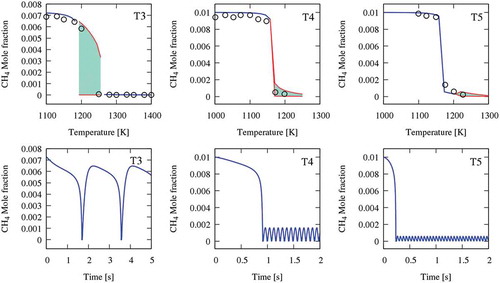
Figure 2. Methane oxidation in a JSR at P = 1.1 atm, τ = 0.5 s, and φ = 1 diluted with 90% of N2. Oscillation ranges are highlighted with the filled pattern.

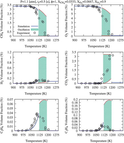
Figure 3. Range of temperature oscillations (ΔT = T-T_in) and CH₄ conversion versus inlet temperature, for the different dilution systems.

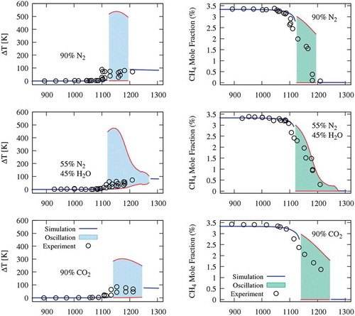
Figure 4. Temperature and CH₄ profiles at 1185 K, in CO₂ diluted system. Temperature and methane profile close to the peak temperature (right panel).

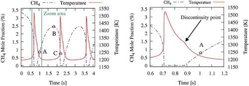
Figure 5. Sensitivity analysis of methane concentration in the CO₂ diluted system and T_in = 1185 K (points A, B and C are shown in Figure 4).

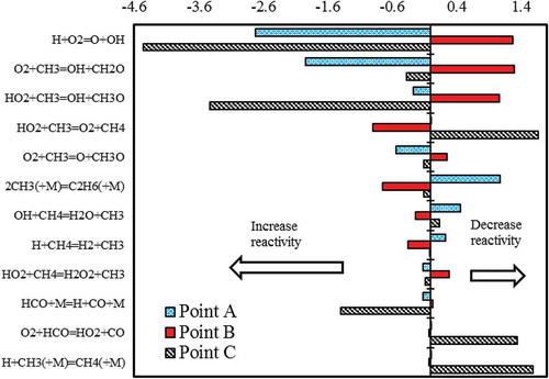
Figure 6. First derivatives of CH₄ and O₂ profiles of the CO₂ diluted system and T_in = 1185 K.

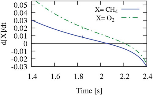
Figure 7. CH₄ conversion at 1185 K, CO₂ dilution. Profile of major species.

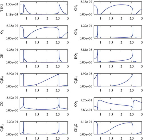
Figure 8. Oscillations of temperature and CH₄ concentration in CO₂ diluted systems. T_in = 1140 K (black line); T_in = 1185 K (dotted-dashed line); T_in = 1245 K (red line).

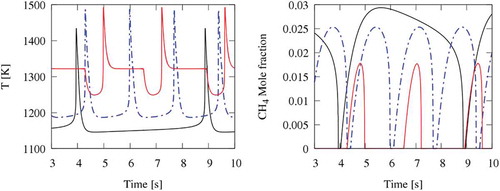
Figure 9. Oscillations of temperature and CH₄ concentration in N₂, CO₂, and (N₂+H₂O) diluted systems. CO₂ (black lines); N₂ (dotted-dashed lines); N₂+H₂O (red lines).

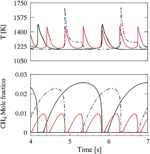
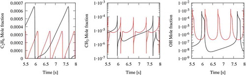
Figure 10. Comparison between cyclic oscillations in N₂+H₂O (red lines) and CO₂ diluted systems (black lines). C₂H₆, CH3, and OH concentration profiles.

de Joannon, M., Sabia, P., Tregrossi, A., and Cavaliere, A. 2004. Dynamic behavior of methane oxidation in premixed flow reactor. Combust. Sci. Technol., 176(5–6), 769–783. doi:10.1080/00102200490428387.

 Web of Science ®Google Scholar

De Joannon, M., Cavaliere, A., Faravelli, T., Ranzi, E., Sabia, P., and Tregrossi, A. 2005. Analysis of process parameters for steady operations in methane mild combustion technology. Proc. Combust. Inst., 30(2), 2605–2612. doi:10.1016/j.proci.2004.08.190.

 Web of Science ®Google Scholar

El Bakali, A., Dagaut, P., Pillier, L., Desgroux, P., Pauwels, J.F., Rida, A., and Meunier, P. 2004. Experimental and modeling study of the oxidation of natural gas in a premixed flame, shock tube, and jet-stirred reactor. Combust. Flame, 137(1–2), 109–128. doi:10.1016/j.combustflame.2004.01.004.

 Web of Science ®Google Scholar

Le Cong, T., Dagaut, P., and Dayma, G. 2008. Oxidation of natural gas, natural gas/syngas mixtures, and effect of burnt gas recirculation: experimental and detailed kinetic modeling. J. Eng. Gas Turb. Power, 130(4), 41502. doi:10.1115/1.2901181.

 Web of Science ®Google Scholar