Improvement of heat- and mass transfer modeling for single iron particles combustion using resolved simulations

Figures & data

Figure 1. Boundary layer resolved geometry (Thijs et al. 2022).

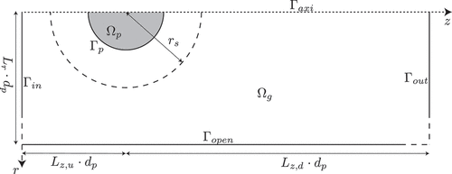
Figure 2. Comparison of numerically obtained Nusselt numbers and Nusselt numbers obtained with correlations from literature. Note, constant material properties at $300\mathrm{K}$ are used.

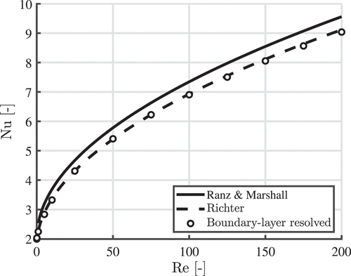
Figure 3. Nusselt correlation for different reference temperatures. Line represent either a hot gas flow (with markers) or a cold gas flow (without markers) past a iron particle with a particle diameter $d_{\mathrm{p}}=50$ m. Temperature differences between the gas and the particle are: 10 K (solid line), 1200 K (dotted line) and 2200 K (dashed line).

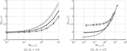
Figure 4. Boundary-layer resolved obtained Nusselt numbers and different correlations.

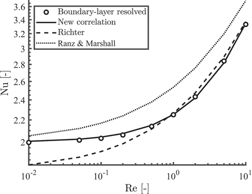
Figure 5. Temperature profiles for a $50$ µm particle burning in (a) Nitrogen and (b) Argon with $X_{{\mathrm{O}}_2}=0.21$. Temperature profiles are compared between the boundary layer resolved model (markers) and the Lagrangian particle model (line). The solid lines are obtained with the Nusselt and Sherwood correlations as proposed by Equations (17)(17) $\mathrm{N}\mathrm{u}=2+\left(0.02\mathrm{P}{\mathrm{r}}^{1/3}\mathrm{R}{\mathrm{e}}^{1/2}+0.33\mathrm{P}{\mathrm{r}}^{1/3}\mathrm{R}{\mathrm{e}}^{2/3}\right)\mathrm{\Phi },$(17) and (18(18) $\mathrm{S}\mathrm{h}=2+\left(0.02\mathrm{S}{\mathrm{c}}^{1/3}\mathrm{R}{\mathrm{e}}^{1/2}+0.33\mathrm{S}{\mathrm{c}}^{1/3}\mathrm{R}{\mathrm{e}}^{2/3}\right)\mathrm{\Phi },$(18) ), while the dashed line is obtained with the Ranz- Marshall correlations and the 1/3-rule.

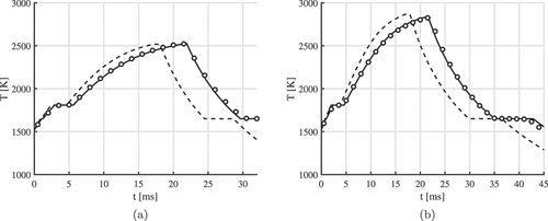
Table 1. Comparison between the boundary-layer resolved model (BLR) and the Lagrangian particle model (0D) for a $50$ µm particle burning in ${\mathrm{O}}_2$ – ${\mathrm{N}}_2$. We distinguish between the new proposed method (new correlation and $A_{\mathrm{f}}=1/2$) and the previous used methods (Ranz-Marshall and $A_{\mathrm{f}}=1/3$).

$X_{{\mathrm{O}}_2}$	Model	$t_{\mathrm{m}\mathrm{a}\mathrm{x}}$ [ms]	$T_{\mathrm{m}\mathrm{a}\mathrm{x}}$ [K]	$\mathrm{F}\mathrm{e}$ evap [%]
$0.13$	BLR	$38.9$	$1898$	$2.6\cdot {10}^{-3}$
	$1/2$ film	$38.1$	$1883$	$2.5\cdot {10}^{-3}$
	$1/3$ film	$31.8$	$1875$	$2.4\cdot {10}^{-3}$
$0.17$	BLR	$27.9$	$2251$	$5.2\cdot {10}^{-2}$
	$1/2$ film	$27.6$	$2231$	$4.8\cdot {10}^{-2}$
	$1/3$ film	$22.9$	$2233$	$4.8\cdot {10}^{-3}$
$0.21$	BLR	$21.3$	$2524$	$0.32$
	$1/2$ film	$21.2$	$2508$	$0.32$
	$1/3$ film	$17.6$	$2518$	$0.34$
$0.26$	BLR	$16.2$	$2784$	$1.24$
	$1/2$ film	$16.0$	$2769$	$1.30$
	$1/3$ film	$13.2$	$2783$	$1.41$
$0.31$	BLR	$13.1$	$2967$	$2.85$
	$1/2$ film	$12.5$	$2954$	$2.9$
	$1/3$ film	$10.3$	$2967$	$3.15$

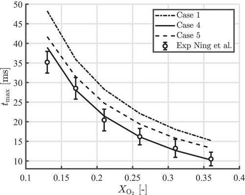
Table 2. Summary of test cases used to investigate the effect on $t_{\mathrm{m}\mathrm{a}\mathrm{x}}$.

Case	$A_{\mathrm{f}}$	$\rho =\mathrm{f}(T)$	Slip velocity	Stefan flow
1	1/2	no	no	no
2	1/2	yes	no	no
3	1/2	yes	yes	no
4	1/2	yes	yes	yes
5	1/3	no	no	no

Figure 6. Effect of different modeling strategies on $t_{\mathrm{m}\mathrm{a}\mathrm{x}}$, the cases are summarized in Table 2.

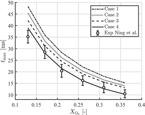
Figure 7. Effect of reference temperature on the temperature profile for a $50$ µm particle burning $X_{{\mathrm{O}}_2}$. The results are shown for case 1, 4 and 5, the cases are summarized in Table 2.

Thijs, L. C., C. E. A. G. van Gool, W. J. S. Ramaekers, J. A. van Oijen, and L. P. H. de Goey. 2022. Resolved simulations of single iron particle combustion and the release of nanoparticles. Proc Combust Inst. Under Review.

 Web of Science ®Google Scholar