Temperature Stratification Induced Ignition Regimes for Gasoline Surrogates at Engine-Relevant Conditions

Figures & data

Figure 1. A schematic presentation of the combustion process shows, a) hotspot/coolspot initial T profile, b) centered ignition and regular propagation inside the hotspot/coolspot, c) off-centered primary ignition due to NTC and double ignition front propagation, and d) occurrence of primary ignition and subsequently, formation of the secondary ignition kernel due to NTC.

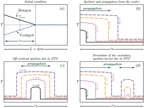
Figure 2. PRF and PRF-E ignition delay time versus temperature profiles at P = 20 and 50 bar, black circles are marking the locations of the studied cases.

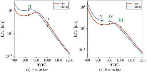
Table 1. Conditions for the five cases: pressure, average temperature, IDT, excitation time, IDT gradient versus temperature, acoustic speed, and constant volume pressure.

	Fuel	P[bar]	${\mathbf{T}}_{\mathit{ave}}$[K]	${\tau }_{\mathit{i}}$[ms]	${\tau }_{\mathit{e}}$[$\mathit{\mu }$s]	$\mathit{\alpha }$[s/K]	${\mathbf{U}}_a$[m/s]	${\mathbf{P}}_{\mathit{cv}}$[bar]
Case I	PRF	20	1000	2.9	9	4.6e-5	589.23	67.44
	PRF-E	20	1000	2.2	13	3.5e-5	589.61	67.07
Case II	PRF	20	830	6.7	11	2.2e-5	539.98	78.86
	PRF-E	20	830	11	11	1.4e-5	540.36	78.66
Case III	PRF	50	1000	1.2	7	1.3e-5	589.23	170.71
	PRF-E	50	1000	0.9	8	1.2e-5	589.61	170.30
Case IV	PRF	50	900	1.6	9	4.5e-6	560.75	186.79
	PRF-E	50	900	2.2	10	4.7e-6	561.13	186.11
Case V	PRF	50	830	1.5	8	2.5e-6	539.98	199.56
	PRF-E	50	830	2.3	11	5.0e-6	540.36	199.68

Table 2. Conditions for the five cases: pressure, average temperature, energy density, von-Neumann pressure, detonation equilibrium pressure, CJ velocity, and induction length ratio.

	Fuel	P[bar]	${\mathbf{T}}_{\mathit{ave}}$[K]	${\mathbf{E}}_c$[MJ/m^3]	${\mathbf{P}}_{\mathit{znd}}$[bar]	${\mathbf{P}}_{\mathit{cj}}$[bar]	${\mathbf{U}}_{\mathit{cj}}$[m/s]	L1/L2
Case I	PRF	20	1000	19.52	219.5	123.1	1841.74	0.033
	PRF-E	20	1000	19.45	218.9	122.5	1840.97	0.039
Case II	PRF	20	830	23.36	263.6	145.8	1841.70	0.031
	PRF-E	20	830	23.28	262.9	145.5	1840.98	0.041
Case III	PRF	50	1000	48.80	560.3	312.1	1862.07	0.039
	PRF-E	50	1000	48.63	558.7	311.4	1861.20	0.050
Case IV	PRF	50	900	54.00	620.6	343.6	1860.65	0.045
	PRF-E	50	900	53.82	618.9	342.9	1859.81	0.060
Case V	PRF	50	830	58.40	671.6	370.1	1859.80	0.055
	PRF-E	50	830	58.20	669.8	369.3	1858.97	0.077

Figure 3. Ignition regime diagram of case I ($\mathit{P}$ = 20 bar and $T_{\mathit{ave}}$ = 1000 K), red zone indicates the detonation peninsula of a) PRF and b) PRF-E mixtures, respectively. Colored circles display the hotspot pressure calculated for each 1D simulation. Letters P, B, and N indicate supersonic ignition, subusonic ignition and the nominal condition for knock initiation inside SI engines (Kalghatgi et al. 2009). c) IDT distribution at the initial time versus T of PRF and PRF-E mixtures.

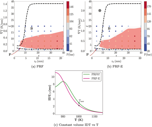
Figure 4. Ignition regime diagram of case II ($\mathit{P}$ = 20 bar and $T_{\mathit{ave}}$ = 830 K), red zone indicates the detonation peninsula of a) PRF and b) PRF-E mixtures, respectively. Colored circles display the hotspot pressure calculated for each 1D simulation. Letters P, B, and N indicate supersonic ignition, subusonic ignition and the nominal condition for knock initiation inside SI engines (Kalghatgi et al. 2009). c) IDT distribution at the initial time versus T of PRF and PRF-E mixtures.

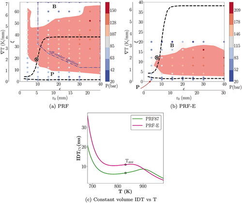
Figure 5. Ignition regime diagram of case III ($\mathit{P}$ = 50 bar and $T_{\mathit{ave}}$ = 1000 K), red zone indicates the detonation peninsula of a) PRF and b) PRF-E mixtures, respectively. Colored circles display the hotspot pressure calculated for each 1D simulation. Letters P, B, and N indicate supersonic ignition, subusonic ignition and the nominal condition for knock initiation inside SI engines (Kalghatgi et al. 2009). c) IDT distribution at the initial time versus T of PRF and PRF-E mixtures.

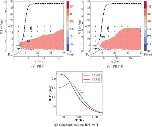
Figure 6. Ignition regime diagram of case I ($\mathit{P}$ = 50 bar and $T_{\mathit{ave}}$ = 900 K), red zone indicates the detonation peninsula of a) PRF and b) PRF-E mixtures, respectively. Colored circles display the hotspot pressure calculated for each 1D simulation. Letters P, B, and N indicate supersonic ignition, subusonic ignition and the nominal condition for knock initiation inside SI engines (Kalghatgi et al. 2009). c) IDT distribution at the initial time versus T of PRF and PRF-E mixtures.

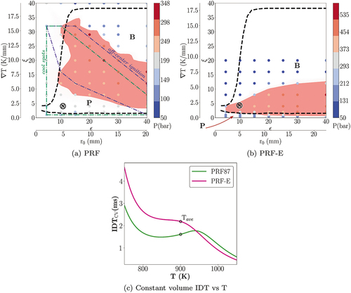
Figure 7. Ignition regime diagram of case V ($\mathit{P}$ = 50 bar and $T_{\mathit{ave}}$ = 830 K), red zone indicates the detonation peninsula of a) PRF and b) PRF-E mixtures, respectively. Colored circles display the hotspot pressure calculated for each 1D simulation. Letters P, B, and N indicate supersonic ignition, subusonic ignition and the nominal condition for knock initiation inside SI engines (Kalghatgi et al. 2009). c) IDT distribution at the initial time versus T of PRF and PRF-E mixtures.

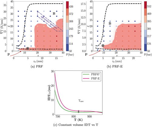
Figure 8. Predicted detonation peninsula of case I and II using the second method, i.e. The contours depict the maximum hotspot pressure normalized by the von Neumann pressure. Letters P, and B indicate supersonic ignition and subusonic ignition regimes.

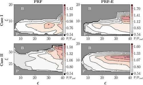
Figure 9. Predicted detonation peninsula of case III-V using the second method, i.E. The contours depict the maximum hotspot pressure normalized by the von Neumann pressure. Letters P, and B indicate supersonic ignition and subusonic ignition regimes.

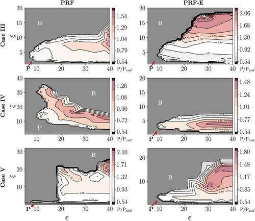
Table 3. Pressure intensity levels at the nominal point location and inside the detonation peninsula for case I-V. Additionally, the table shows the degree of the NTC behavior observed in 1D simulations for case I-V.

	Fuel	P[bar]	Tave[K]	$\mathrm{\Delta }{P}_N$ [bar]	$\mathrm{\Delta }{P}_D$ [bar]	NTC effect
Case I	PRF	20	1000	<0	20-80	No
	PRF-E	20	1000	<0	20-100	No
Case II	PRF	20	830	30	10-70	Mild
	PRF-E	20	830	30	20-90	Mild
Case III	PRF	50	1000	90	90-190	No
	PRF-E	50	1000	<0	90-260	No
Case IV	PRF	50	900	<0	40-160	High
	PRF-E	50	900	120	60-350	No
Case V	PRF	50	830	80	50-236	Mild
	PRF-E	50	830	120	100-350	No

Figure 10. Locations of selected points on PRF mixture regime diagram for transient analysis at 50 bar and 900 K, case IV.

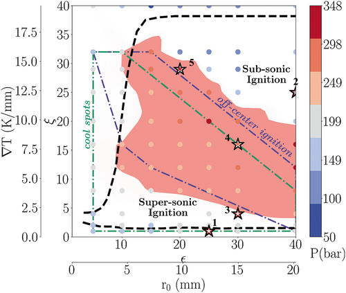
Figure 11. Transient profiles of temperature and normalized pressure at point 1 for PRF mixture at case IV (T = 900 K and P = 50 bar), demonstrating supersonic ignition propagation.

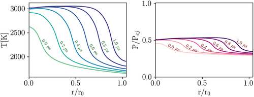
Figure 12. Transient profiles of temperature and normalized pressure at point 2 for PRF mixture at case IV (T = 900 K and P = 50 bar), demonstrating subsonic ignition propagation.

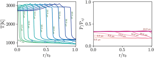
Figure 13. Transient profiles of temperature and normalized pressure at point 3 for PRF mixture at case IV (T = 900 K and P = 50 bar), demonstrating detonation development.

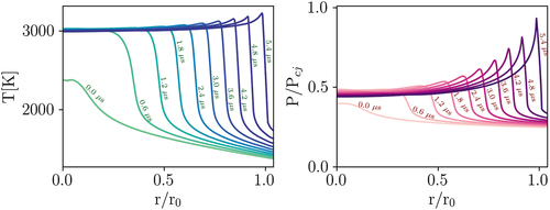
Figure 14. Transient profiles of temperature and normalized pressure at point 4 for PRF mixture at case IV (T = 900 K and P = 50 bar), demonstrating occurrence of off-centered ignition.

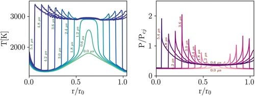
Figure 15. Transient profiles of temperature and normalized pressure at point 5 for PRF mixture at case IV (T = 900 K and P = 50 bar), demonstrating appearance of secondary ignition.

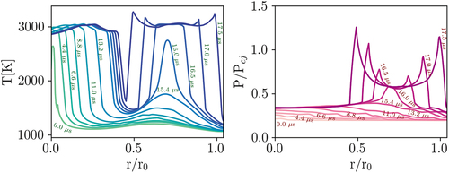
Table A1. Test case configuration.

${\rho }_{\mathit{l}}$ [Kg/m^3]	${\rho }_{\mathit{r}}$ [Kg/m^3]	Pl [pa]	Pr [pa]	U [m/s]	MW	L [m]	Gridpoints
1	0.125	1	0.1	0	28.9	1	200-800

Figure A1. Sod’s shocktube pressure, velocity, density and acoustic speed distribution versus analytical solution at 0.1644 s.

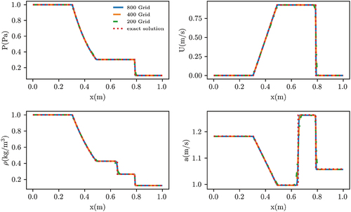
Table A2. Test case configuration.

Tave [K]	$\mathrm{\nabla }\mathit{T}$ [K/m]	P0 [atm]	rhs [m]	$\mathit{\xi }$	L [m]	$\mathrm{\Delta x}$ [m]	UCJ [m/s]	HRL [m]
1381	1000	40	0.008	1	0.04	8e^−7	1834	3e^−5

Figure A2. Temperature profiles (dashed lines are from (Pan et al. 2019), solid lines are from the present work) and reaction, pressure fronts speeds for methane hotspot detonation, $P_0=40$ atm, $T_{\mathit{ave}}=1381$ K, $\mathrm{\nabla T}=1$ K/mm, $r_0=8$ mm. CJ speed is calculated at $T_{\mathit{ave}}$ using SDToolbox (Kao and Shepherd 2008).

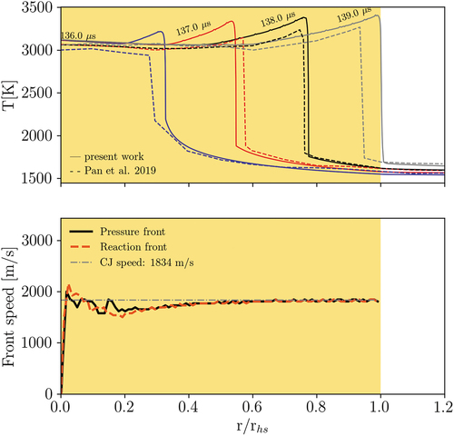
Table A3. Grid sensitivity case configuration.

Tave [K]	$\mathrm{\nabla }\mathit{T}$ [K/m]	P0 [bar]	R0 [m]	$\mathit{\xi }$	$\mathit{\epsilon }$	L [m]	$\mathrm{\Delta x}$ [$\mathit{\mu }$m]	HRL [m]
1000	502	50	0.004	4	10	0.04	0.5, 0.75, 1	1e^−5

Figure A3. Mesh sensitivity study for case.Black dashed-line result from grid size = $1\text{mum}$, Blue solid line results from grid size = 0.75 $\text{mum}$, red dashed-line results from grid size = 0.5$\text{mum}$.

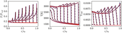
Figure B1. The ZND detonation structures of case I-V for PRF and PRF-E mixtures. The blue lines depict the heat release profiles, and the red-dashed lines depict the temperature profiles. L1 and L2 indicate the first and second induction lengths, respectively.

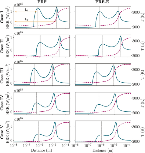
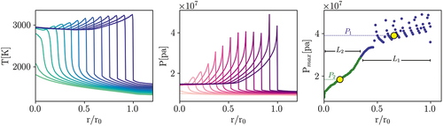
Figure C1. Transient temperature and pressure profiles as well as distribution of maximum pressure for a hotspot detonation scenario. Clusters are separated by colors. Yellow circles indicate the mean value calculated for each cluster.

Kalghatgi, G., D. Bradley, J. Andrae, and A. Harrison (2009), The nature of ‘super- knock’and its origins in si engines. ‘IMechE conference on internal combustion engines: performance fuel economy and emissions’ London, 8–9.

 Google Scholar

Pan, J., S. Dong, H. Wei, T. Li, G. Shu, and L. Zhou. 2019. Temperature gradient induced detonation development inside and outside a hotspot for different fuels. Combust. Flame 205:269–77. doi:10.1016/j.combustflame.2019.04.003.

 Web of Science ®Google Scholar

Kao, S., and J. Shepherd (2008). Numerical solution methods for control volume explosions and znd detonation structure. Galcit report fm 2006. 7, 1–46.

 Google Scholar