Cycling on the edge: the effects of edge lines, slanted kerbstones, shoulder, and edge strips on cycling behaviour of cyclists older than 50 years

Figures & data

Table 1. Participants’ demographic characteristics.

Experiment	Bicycle	N	% Male	Age (in years)	Weekly cycled km
Exp. 1	Conventional	17	70.6	M = 66.5, SD = 8.0	M = 34.4, SD = 26.5
	Electric	15	40.0	M = 70.2, SD = 9.8	M = 61.1, SD = 59.8
	Total	32	56.3	M = 68.3, SD = 9.0	M = 46.5, SD = 45.9
Exp. 2	Conventional	20	50.0	M = 61.6, SD = 5.1	M = 78.4, SD = 70.9
	Electric	10	60.0	M = 65.5, SD = 7.2	M = 79.5, SD = 54.7
	Total	30	53.3	M = 62.9, SD = 6.1	M = 78.7, SD = 65.0

Figure 1. All conditions from Experiment 1. (A) Edge Lines, (B) White Slanted Kerbstones, (C) Grey Artificial Grass Strips, (D) Green Artificial Grass Strips, (E) Concrete Street-print Strips, (F) Control Location 1, (G) Control Location 2.

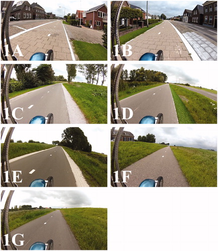
Table 2. Experimental conditions properties.

Condition	Order		Distance in-between (m)		Treatment length (m)		Sampling stretch (m)		Path width (m)		Strip width (cm)
Outbound/Return	O	R	O	R	O	R	O	R	O	R
SK	–	7	–	–	–	90	–	85	–	2.5	–
ELC	1	6	525	0	90	50	85	50	2.5	2.3	–
CL 1	2	5	1650	450	1600	1600	85	85	2.3	2.3	–
Grey AGS	3	4	0	1650	225	225	85	85	3.0	3.0	50
Green AGS	4	3	0	0	75	75	75	75	3.0	3.0	50
CSS	5	2	0	0	150	150	85	85	3.0	3.0	50
CL 2	6	1	0	0	575	575	85	85	3.0	3.0	–
ELI 5 cm	2	4	45	0	450	450	102	102	3.5	3.5	–
ELI 15 cm	3	3	0	45	950	590	102	102	3.5	3.5	–
ELC 15 cm	4	2	0	0	135	510	102	102	3.5	3.5	–
WCES	5	1	0	0	340	340	102	102	3.5	3.5	30
CL 3	1	5	0	–	100	100	91	91	3.5	3.5	–

AGS: Artificial Grass Strip; CL: Control Location; CSS: Concrete Street-print Strip; ELC: Edge Line Continuous; ELI: Edge Line Intermittent; SK: Slanted Kerbstones; WCES: White Chippings Edge Strip.

Figure 2. All conditions from Experiment 2. (A) Intermittent Edge Lines 5 cm, (B) Intermittent Edge Lines 15 cm, (C) Continuous Edge Lines 15 cm, (D) 30 cm White Chippings Edge Strip, (E) Control Location 3.

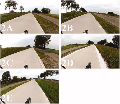
Figure 3. The lateral position measurement process with VLC Media Player™ and JRuler Pro™. In this example, the lateral position is measured and calculated as 75 cm + 12 cm = 87 cm.

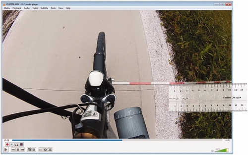
Figure 4. A schematic representation of the conditions for Experiment 1 (left: 1A = Edge Line, 1B = Slanted Kerbstones, 1C = Grey Artificial Grass, 1D = Green Artificial Grass, 1E = Street-print, 1F = Control Location 1, 1G = Control Location 2) and Experiment 2 (right: 2A = Intermittent Edge Lines 5 cm, 2B = Intermittent Edge Lines 15 cm, 2C = Continuous Edge Lines 15 cm, 2D = White Chippings Edge Strip, 2E = Control Location 3). The notch represents the edge of the path that was used to measure the lateral position.

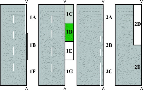
Figure 5. The average lateral position (in cm) per condition: 0 = right hand cycle path edge as indicated in Figure 4. The error bars represent the standard error of the mean (S.E.).

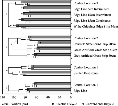
Figure 6. The average SDLP (in cm) per condition. The error bars represent the standard error of the mean (S.E.).

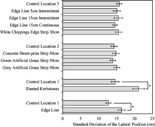
Table 3. Descriptive statistics and non-parametric test results for the differences between users of conventional and electric bicycles, collapsed over all conditions.

Experiment	Variable	Mean (± SD) Conventional	Mean (± SD) Electric	U	Z	p	r
Exp. 1	Lateral Position	67.88 ± 15.57	68.81 ± 14.59	127	−0.02	.99	0.00
	SDLP	16.48 ± 3.73	14.39 ± 4.09	81	−1.76	.08	0.31
	Speed	18.05 ± 2.99	17.76 ± 2.08	106	−0.52	.61	0.09
Exp. 2	Lateral Position	76.54 ± 15.70	87.58 ± 10.31	54	−2.02	.04	0.37
	SDLP	15.01 ± 3.90	15.89 ± 1.86	78	−0.97	.33	0.18
	Speed	17.59 ± 2.59	18.63 ± 2.55	75	−1.10	.27	0.20

Table 4. The results for the pairwise effects on lateral position for the conditions in Experiment 1 and 2.

Condition	Z	df	p	r
Edge Lines – White	−4.94	1	<.001	0.87
Slanted Kerbstones – White	−4.56	1	<.001	0.81
Artificial Grass Strip – Grey	−4.45	1	<.001	0.79
Artificial Grass Strip – Green	−4.49	1	<.001	0.79
Concrete Street-print Strip	−4.77	1	<.001	0.84
Edge Line 5 cm Intermittent	−2.40	1	.017	0.44
Edge Line 15 cm Intermittent	−1.16	1	.245	0.21
Edge Line 15 cm Continuous	−0.11	1	.910	0.02
White Chippings Edge Strip	−3.57	1	<.001	0.65

Bonferroni corrected α = .0055.

All effects are comparisons with the control conditions.

Table 5. Lateral position effects of bicycle type for each condition in Experiment 2.

Location	Mean (± SD) Conventional	Mean (± SD) Electric	U	W	Z	p	r
White Chippings Edge Strip 30 cm	83.56 ± 15.96	96.42 ± 13.82	53	263	−2.07	.039	0.38
Edge Line 15 cm Continuous	75.16 ± 17.14	87.35 ± 12.69	47	257	−2.33	.020	0.43
Edge Line 15 cm Intermittent	74.44 ± 18.09	83.61 ± 9.61	61	271	−1.72	.086	0.31
Edge Line 5cm Intermittent	73.44 ± 16.87	82.89 ± 13.45	64	274	−1.58	.113	0.29
Control Location 3	76.07 ± 15.40	87.62 ± 11.08	53	263	−2.07	.039	0.38

Bonferroni corrected α = .01.

Table 6. The results for the pairwise effects on swerving (SDLP) for the conditions in Experiment 1 and 2.

Condition	Z	df	p	r
Edge Lines – White	−3.39	1	.001	0.60
Slanted Kerbstones – White	−3.52	1	<.001	0.62
Artificial Grass Strip – Grey	−0.72	1	.472	0.13
Artificial Grass Strip – Green	−0.44	1	.660	0.08
Concrete Street-print Strip	−0.11	1	.911	0.02
Edge Line 5 cm Intermittent	−1.00	1	.318	0.18
Edge Line 15 cm Intermittent	−0.60	1	.551	0.11
Edge Line 15 cm Continuous	−1.31	1	.192	0.24
White Chippings Edge Strip	−0.36	1	.721	0.07

Bonferroni corrected α = .0055.

All effects are comparisons with the control conditions.

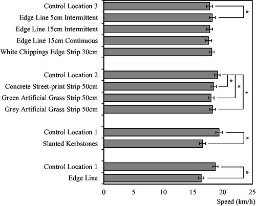
Table 7. The results for the pairwise effects on speed for the conditions in Experiment 1 and 2.

Condition	Z	df	p	r
Edge Lines – White	−4.86	1	<.001	0.87
Slanted Kerbstones – White	−4.86	1	<.001	0.87
Artificial Grass Strip – Grey	−4.31	1	<.001	0.76
Artificial Grass Strip – Green	−4.66	1	<.001	0.82
Concrete Street-print Strip	−3.95	1	<.001	0.70
Edge Line 5 cm Intermittent	−4.20	1	<.001	0.77
Edge Line 15 cm Intermittent	−0.14	1	.885	0.03
Edge Line 15 cm Continuous	−0.66	1	.510	0.12
White Chippings Edge Strip	−1.87	1	.061	0.34

Bonferroni corrected α = .0055.

All effects are comparisons with the control conditions.

Table 8. Mann–Whitney U significant test results (α ≤ .0055) for the effects of bicycle type on the Ipsative Scores of Speed per Treatment.

Treatment	M (±SD) conventional	M (±SD) electric	U	z	p	r
Green AGS	−1.53 (±1.10)	−0.52 (±0.46)	45.0	−3.12	.002	−0.51
Street-print	−0.98 (±0.72)	−0.21 (±0.46)	32.5	−3.59	<.001	−0.54

Bonferroni corrected α = .0055.

The Ipsative Scores are the difference scores per Treatment (i.e. Treatment – Control Condition).

Table 9. Subjective opinions in percentages for the treatments in Experiment 1.

Treatment	Remembered after presentation	Positive	Neutral	Negative	Weighed κ
Grey Artificial Grass Strip	50.0	36.7	30.0	33.3	0.89
Green Artificial Grass Strip	84.4	38.7	29.0	32.3	0.55
Concrete Street-print Strip	56.3	38.7	25.8	35.5	0.72

The evaluations include all participants and not only who remembered the intervention.

Table 10. Subjective opinions in percentages for the treatments in Experiment 2.

Treatment	Remembered after presentation	Very helpful	Rather helpful	Not helpful
No Line (Control Condition)	90.0	33.3	33.3	33.3
Edge Line 5–15 cm Intermittent	90.0	44.4	48.1	7.4
Edge Line 15 cm Continuous	80.0	91.7	8.3	0.0
White Chippings Edge Strip 30 cm	100.0	86.7	10.0	3.3

The evaluations include all participants and not only who remembered the intervention.

Figure 7. The average cycling speed (km/h) per condition. The error bars represent the standard error of the mean (S.E.).

Table

Procedure Post-ride Interviews Experiment 1

1. Short verbal introduction of the area where the treatment was applied.

2. Question: ‘Can you remember this area?’

If yes: the researcher continues with question 3.

If no: the researcher shows a picture of the treatment and continues with question 3.

3. Question: ‘Could you describe what you have seen there?’

4. The researcher shows the video of the participant cycling past the modifications.

5. Question: ‘Could you describe your first reaction when you saw these modifications?’

6. Question: ‘What is your opinion about these modifications?’

Procedure Post-ride Interviews Experiment 2

1. Researcher shows photo of the treatment location.

2. Question: ‘Can you remember this section?’

3. Question: ‘What do you think about this measure in general?’

4. The researcher monitors and writes down whether the participant’s opinion is positive or negative.

5. Question: ‘To what extent do you believe that these modifications contribute to keeping cyclists on the cycle path?’

6. Question after all treatments were discussed: ‘Do you have a preference for one of the treatments?’

Table

Exclusion criterion	Measures	Experiment	Condition(s)	N	Freq.
Overtaking	LP, SDLP, and Speed	1	ELC	1	1
			SK	1	1
			Grey AGS	2	2
			Green AGS	3	3
			CL 1	1	1
			CL 2	1	1
		2	ELI 5cm	1	1
			ELC 15cm	2	2
			WCES	1	1
			CL 3	1	1
Entering Strip(s)	LP, SDLP, and Speed	1	Grey AGS	2	2
			Green AGS	4	5
			CSS	3	3
		2	WCES	1	1
Speed Obstruction	Speed	1	CL 1	1	1