Infinite horizon cancer treatment model with isoperimetrical constraint: existence of optimal solutions and numerical analysis

Figures & data

Table 1. Parameter set used in Schättler and Ledzewicz (2015) for the corresponding finite horizon model.

Coefficient	a 1	a 2	a 3	u max	v max	θ1	θ2	q 1	q 2	q 3	c 1	c 2
Value	0.197	0.395	0.107	0.95	0.30	1	0.01	1	1	1	–	–

Table 2. Parameter set for the infinite horizon model presented here

Coefficient	a 1	a 2	a 3	u max	v max	θ1	θ2	q 1	q 2	q 3	c 1	c 2
Value	0.197	0.395	0.107	0.95	0.30	1	0.01	1	1	1	1	0.01

Figure 1. States for a sufficient large budget and initial state N(0) = (10, 10, 10).

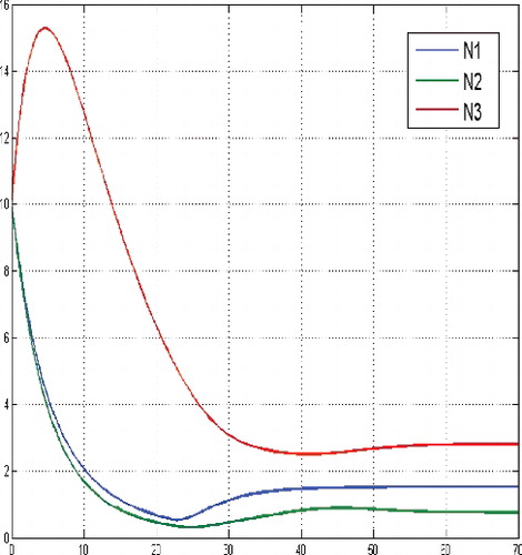
Figure 2. Controls for a sufficient large budget and initial state N(0) = (10, 10, 10).

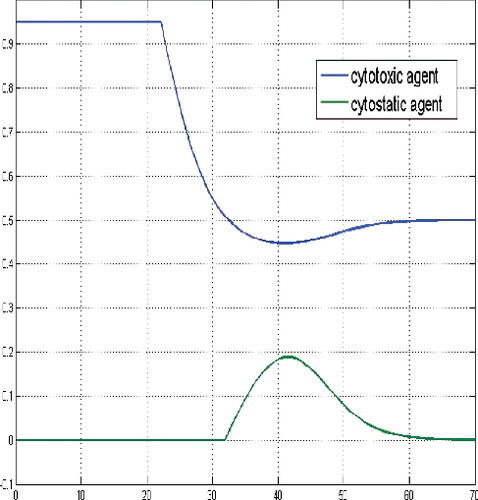
Figure 3. Adjoint functions for a sufficient large budget and initial state N(0) = (10, 10, 10).

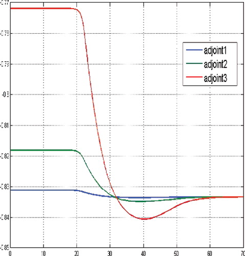
Figure 4. States for a sufficient large budget and large initial tumor cells population, i.e. N(0) = (30, 30, 30).

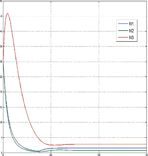
Figure 5. Controls for a sufficient large budget and large initial tumour cells population, i.e. N(0) = (30, 30, 30).

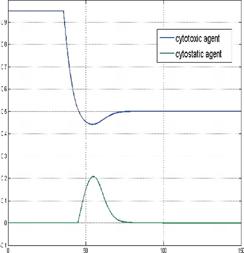
Figure 6. Adjoint functions for a sufficient large budget and large initial tumour cells population, i.e. N(0) = (30, 30, 30).

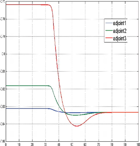
Figure 7. States for a sufficient large budget and N(0) = (1, 1, 1).

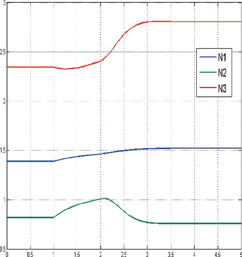
Figure 8. Controls for a sufficient large budget and N(0) = (1, 1, 1).

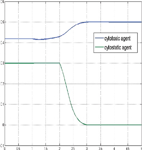
Figure 9. Adjoint functions for a sufficient large budget and N(0) = (1, 1, 1).

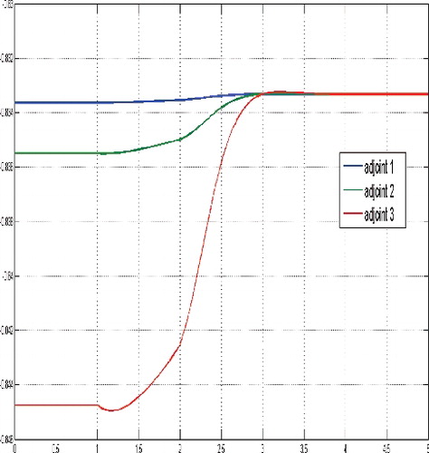
Figure 10. States for a sufficient large budget and initial state near the equilibrium level, here N(0) = (3, 3, 3).

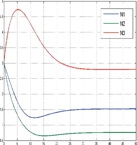
Figure 11. Controls for a sufficient large budget and and initial state near the equilibrium level, here N(0) = (3, 3, 3).

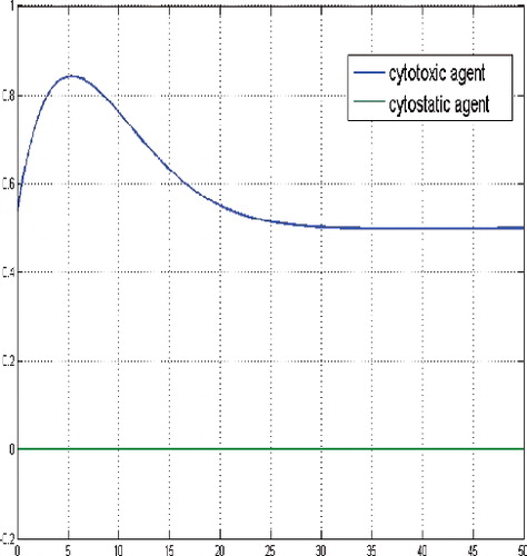
Figure 12. Adjoint functions for a sufficient large budget and and initial state near the equilibrium level, here N(0) = (3, 3, 3).

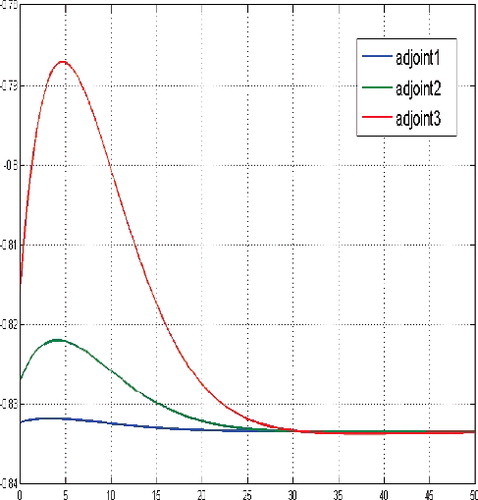
Figure 13. States for a sufficient large budget and a small tumour cells population relatively compared to the level of the equilibrium, N(0) = (0.3866, 0.1722, 0.4412).

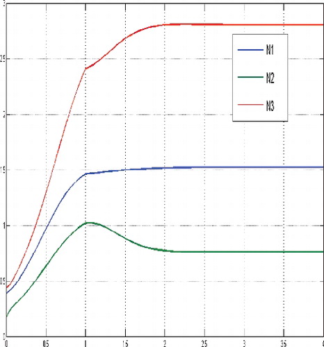
Figure 14. Controls for a sufficient large budget and a small tumour cells population relatively compared to the level of the equilibrium, N(0) = (0.3866, 0.1722, 0.4412).

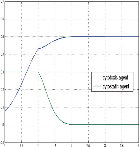
Figure 15. Adjoint functions for a sufficient large budget and a small tumor cells population relatively compared to the level of the equilibrium, N(0) = (0.3866, 0.1722, 0.4412).

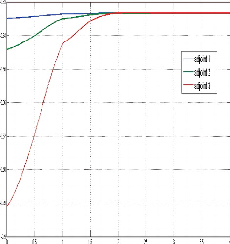
Figure 16. States for small budget d = 100 and N(0) = (10, 5, 10).

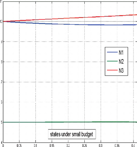
Figure 17. Controls for small budget d = 100 and N(0) = (10, 5, 10).

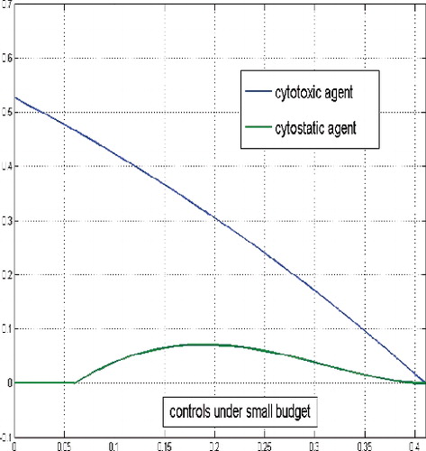
Figure 18. Costates for small budget d = 100 and N(0) = (10, 5, 10).

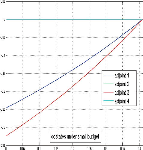
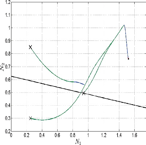
Figure 19.  Phase diagram, slice plane (N ₁,N ₂), case of the threshold budget (long path), d=500.

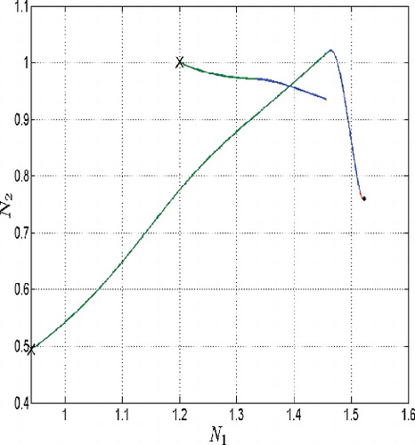
Figure 20.  Phase diagram, slice plane (N ₁,N ₃), case of the threshold budget (long path), d = 500 (long path), d = 500.

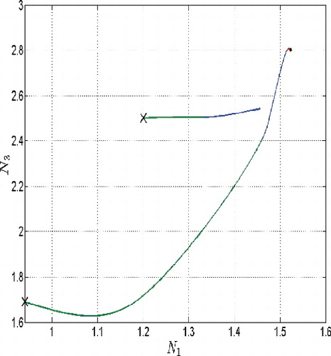
Figure 21. Phase diagra2, slice plane (N ₁,N ₃), case of the (long path), d = 500e threshold budget, d = 500.

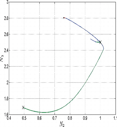
Figure 22.  Phase diagram, slice plane (N ₁,N ₂), case of budget constraint which does not become active (shorter path going near by the equilibrium), d = 500.

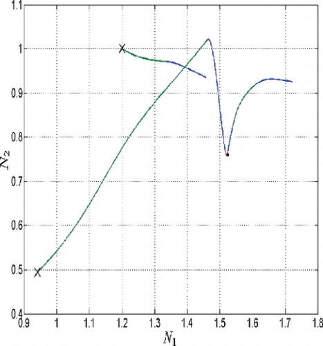
Figure 23.  Phase diagram, slice plane (N ₁,N ₃), case of budget constraint which does not become active (shorter path going near by the equilibrium), d = 500.

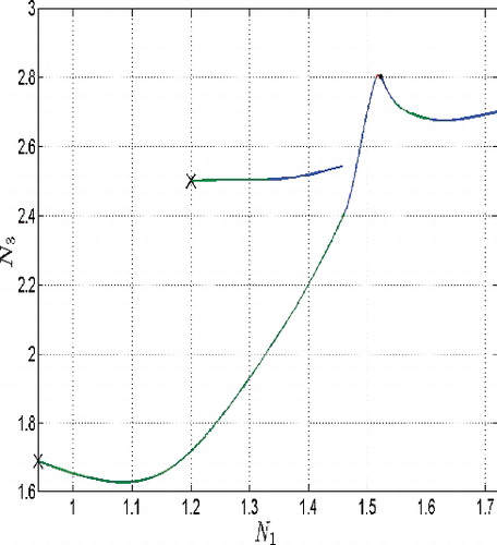
Figure 24.  Phase diagram, slice plane (N ₂,N ₃), case of budget constraint which does not become active (shorter path going near by the equilibrium), d = 500.

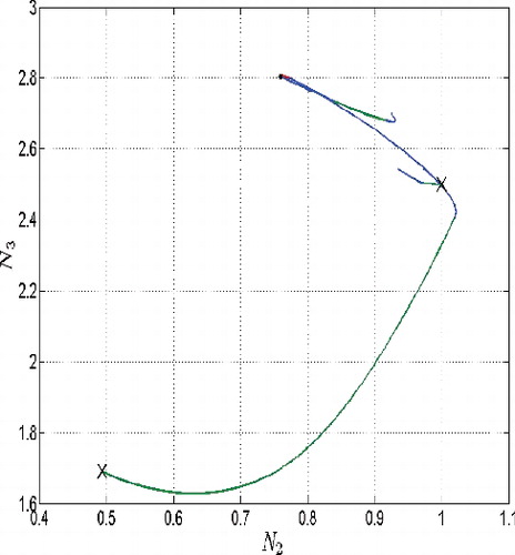
Figure 25. ‘Threshold state trajectories’ for budget d = 500.

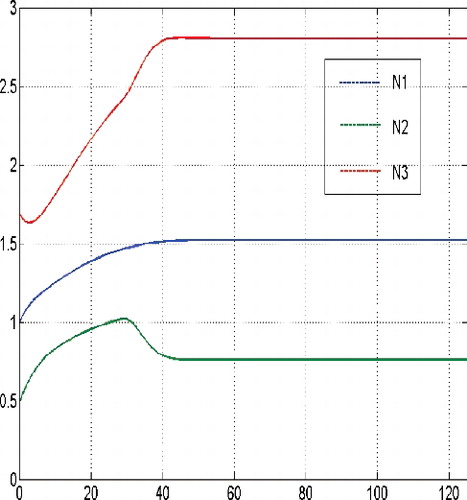
Figure 26. ‘Threshold state trajectories’ for budget d = 500.

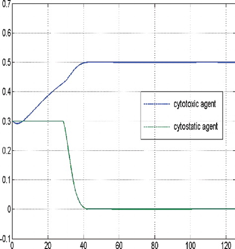
Figure 27. ‘Threshold adjoint functions’ for budget d = 500.

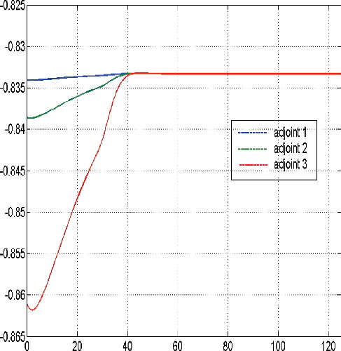
Figure 28. Growth of the budget variable N ₄ for budget d = 500.

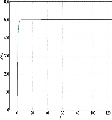
Figure 29. Slice curve for budget d = 500.

Schättler, H. , & Ledzewicz, U . (2015). Optimal control for mathematical models of cancer therapies. An application of geometric methods. Interdisciplinary applied mathematics (Vol. 42). New York, NY: Springer.

 Google Scholar