Efficient path planning for automated guided vehicles using A* (Astar) algorithm incorporating turning costs in search heuristic

Figures & data

Table 1. Overview of control strategies described in the literature that (implicitly) take into account turning costs when using the A${}^{\ast }$ algorithm on a geometric graph.

	A${}^{\ast }$ algorithm used for path planning or routing	Objective of A${}^{\ast }$ algorithm to find shortest-time or shortest-distance path	Decelerations before and accelerations after turning are taken into account in $g(v_s,v_c)$	Separate turning costs taken into account in $g(v_s,v_c)$	Decelerations before and accelerations after turning are taken into account in $h(v_c,v_d)$	Turning taken into account in $h(v_c,v_d)$	Other factors taken into account in $h(v_c,v_d)$ besides those related to turning, distance, or time	Selection of subset or all of successor vertices to evaluate	Admissibility proven	Layout restrictions for using A${}^{\ast }$ algorithm
Heuristic This Paper	Path planning	Time	No	Yes	No	Yes	No	All	Yes	No
Bae and Chung (2018)	Path planning	Time	No	Yes^c	No	No	No	All	No^p	Yes^r
Bae and Chung (2019)	Path planning	Time	No	Yes^c	No	No	No	All	No^p	Yes^r
Ballamajalu et al. (2020)	Path planning	Distance	Unknown^a	Unknown^a	No	Yes^f,g	No	All	No	Yes^r
Chaudhari, Apsangi, and Kudale (2017)	Path planning	Distance	No	Yes^c	No	No	No	All	No^p	Yes^r
Cui et al. (2018)	Routing	Time	Yes^b	Yes^c	Yes^b,d	Yes^c,d,h	No	All	No	Yes^s
Jia et al. (2017)	Routing	Time	Yes^b	No	No	No	No	All	No^p	No^t
Lian and Xie (2019)	Path planning	Time	No	Yes^c	No	No	No	All	No^p	Yes^r
Lian, Xie, and Zhang (2020)	Routing	Time	No	Yes^c	No	No	No	All	No	Yes^r
Lin et al. (2017)	Path planning	Distance	No	No	No	No	Yes^m	All	No^q	No
Liu, Chen, and Huang (2019)	Routing	Distance	Unknown^a	Unknown^a	Yes^e	Yes^c,f	Yes^n	All	No	Yes^r
Liu and Gong (2011) Heuristic 2	Path planning	Distance	No	No	No	No	Yes^m	All	No^q	No^t
Liu and Gong (2011) Heuristic 3	Path planning	Distance	No	No	No	Yes^i	No	All	No	No^t
Mu et al. (2020)	Path planning	Distance	No	No	No	No	No	Subset^o	No	Yes^r
Shi et al. (2020)	Path planning	Distance	No	No	No	Yes^j	No	All	No	No^t
Wang et al. (2015)	Routing	Time	No	Unknown^a	No	No	No	All	No	No^t
Wang and Xiang (2018)	Path planning	Distance	No	Unknown^a	No	Yes^k	No	All	No	Yes^r
Zheng, Xu, and Zheng (2019)	Path planning	Distance	Unknown^a	Unknown^a	No	Yes^l	No	All	No	Yes^r

^a Unspecified how $g(v_s,v_c)$ is computed.

^b Second-order kinematics.

^c Constant amount per turn.

^d Added if current vertex $v_c$ and destination vertex $v_d$ are not at the same horizontal and vertical levels.

^e Seems to be taken into account indirectly as part of turning costs.

^f Added if turn has to be made to reach current vertex $v_c$ from predecessor vertex.

^g Added if obstacles are located in line-of-sight.

^h Deceleration from and acceleration to maximum AGV speed are taken into account in heuristic $h(v_c,v_d)$ when a turn needs to be made.

ⁱ Ratio of two angles is taken into account.

^j Normalised sine and cosine similarity of two vectors are taken into account.

^k A (weighted) cost compensation based on angular deviation is included.

^l One of the (weighted) terms of the heuristic depends on the difference in x- and y-coordinates between current vertex $v_c$, its predecessor vertex, and successor vertex.

^m Heuristic from predecessor of current vertex $v_c$ to destination vertex $v_d$ is included.

ⁿ Also a ‘Repeated route cost’ and ‘Dynamic weight guidance’ are included.

^o The vertices to expand are selected based on differences in x- and y-coordinates between current vertex $v_c$ and destination vertex $v_d$.

^p Heuristic is based on distance or translation time only; proof of admissibility when using Manhattan or Euclidean distance seems to be considered trivial.

^q Lowest-cost path is not always found. The paper acknowledges this.

^r Restricted to orthogonal grids.

^s Restricted to orthogonal and axis-aligned grids. Length of a path segment should at least be equal to the distance required to accelerate from standstill to maximum speed, plus the distance required to decelerate from maximum speed to standstill.

^t Developed for orthogonal grids but does not seem to be a restriction.

Figure 1. Angles of rotation from orientation A to orientation B.

Vertex with two orientations, denoted by A and B. The angle of rotation from A to B in counterclockwise direction is denoted by . The angle of rotation from A to B in clockwise direction is denoted by .

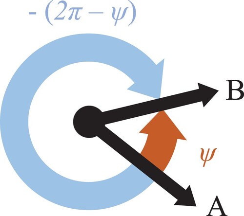
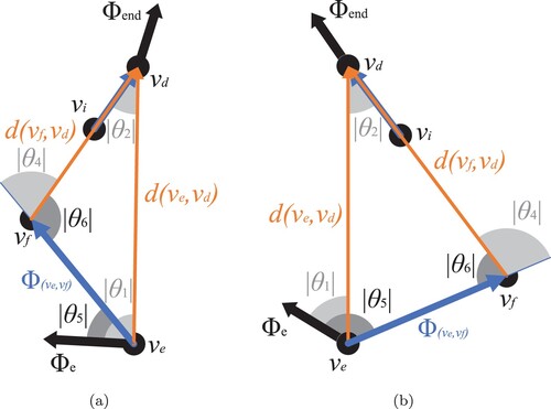
Figure 2. Graphic representation of the minimum absolute angles of rotation $\left|{\theta }_1\right|$, $\left|{\theta }_2\right|$, and $\left|{\theta }_3\right|$ for vertex $v_e$ with specified orientation ${\mathrm{\Phi }}_e$ and destination vertex $v_d$ with end orientation ${\mathrm{\Phi }}_{\mathrm{e}\mathrm{n}\mathrm{d}}$. (a) One incoming edge at $v_d$. The minimum angles of rotation at $v_d$ are equal to $\left|{\theta }_2\right|$ and $\left|{\theta }_3\right|$. (b) One incoming edge at $v_d$. The minimum angles of rotation at $v_d$ are equal to $-\left|{\theta }_2\right|$ and $\left|{\theta }_3\right|$, and (c) two incoming edges a and b at $v_d$.

Read the detailed description of this figure

(a) Vertices , (with, respectively, orientations and ), and are drawn in such a way that the minimum angle of rotation from to Euclidean vector is in counterclockwise direction and equal to , the minimum angle of rotation from to the edge is in counterclockwise direction and equal to , and the minimum angle of rotation from the edge to is in counterclockwise direction and equal to . (b) Vertices (with, respectively, orientations and ), and are drawn in such a way that the minimum angle of rotation from to Euclidean vector is in counterclockwise direction and equal to , the minimum angle of rotation from to the edge is in clockwise direction and equal to , and the minimum angle of rotation from the edge to is in counterclockwise direction and equal to . (c) Vertices (with, respectively, orientations and ), and two predecessor vertices of (i.e. the start vertices of edges and ) are drawn in such a way that the minimum angle of rotation from to Euclidean vector is in counterclockwise direction and equal to , the minimum angles of rotation from to the edges and are, respectively, in clockwise and counterclockwise direction and equal to, respectively, and , and the minimum angles of rotation from the edges and to are, respectively, in clockwise and counterclockwise direction and equal to, respectively, and .

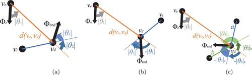
Figure 3. Layout shapes used in the comparative study. (a) Rectangular layout. (b) Hexagonal layout. (c) Arbitrary layout.

Read the detailed description of this figure

(a) Grid layout consisting of square grid elements. The centres of the grid elements are connected to neighbouring grid elements by alternating unidirectional path segments, directed from left to right at the top, and from bottom to top at the left. (b) Grid layout consisting of 9 columns of alternately 9 and 10 hexagonal grid elements. The centres of the grid elements are connected to neighbouring grid elements by alternating unidirectional path segments, directed from top to bottom at the left, from top left to bottom right, and from bottom left to top right. (c) Grid layout consisting of 71 grid elements with an arbitrary convex shape. The centres of the grid elements are connected to neighbouring grid elements by unidirectional path segments, such that the graph is fully connected.

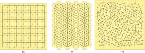
Figure 4. Example layouts with randomly 20% of the grid elements blocked. (a) Rectangular layout. (b) Hexagonal layout. (c) Arbitrary layout.

Read the detailed description of this figure

(a) Grid layout consisting of square grid elements. The centres of the grid elements are connected to neighbouring grid elements by alternating unidirectional path segments, directed from left to right at the top, and from bottom to top at the left. Twenty grid elements in the layout are blocked; these are not connected to neighbouring grid elements. (b) Grid layout consisting of 9 columns of alternately 9 and 10 hexagonal grid elements. The centres of the grid elements are connected to neighbouring grid elements by alternating unidirectional path segments, directed from top to bottom at the left, from top left to bottom right, and from bottom left to top right. Seventeen grid elements in the layout are blocked; these are not connected to neighbouring grid elements. (c) Grid layout consisting of 71 grid elements with an arbitrary convex shape. The centres of the grid elements are connected to neighbouring grid elements by unidirectional path segments, such that the graph is fully connected. Fourteen grid elements in the layout are blocked; these are not connected to neighbouring grid elements.

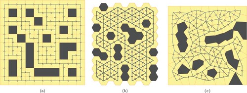
Figure 5. Average number of iterations needed to find one grid element of the lowest-cost path (i.e. path element), for different path lengths, for a $30\times 30$ rectangular grid with $0\mathrm{\%}$ of the grid elements blocked.

2D plot showing the sample mean and 95% confidence interval for the number of iterations per path element, for different path lengths, for the control strategies of Bae and Chung (), modified Cui et al. (), and Heuristic This Paper. An S-curve in the results is visible for all control strategies, starting from bottom left to top right.

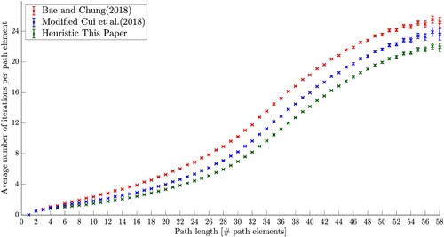
Table 2. Parameter values used for the computations.

Parameter	Value
Maximum (translation) speed, $s_{max}$ (m/s)	2
Size grid element (m)	2
Maximum rotation speed, ${\omega }_{max}$ (rad/s)	$\pi /2$
Start orientation ${\mathrm{\Phi }}_{\mathrm{s}\mathrm{t}\mathrm{a}\mathrm{r}\mathrm{t}}$ of AGV at source vertex $v_s$ (rad)	0

Figure 6. Computed metrics for grids with different element shapes, for different percentages of grid elements blocked, and for different grid sizes. (a) Grid with rectangular elements, with $0\mathrm{\%}$ of the grid elements blocked. (b) Grid with rectangular elements, with $20\mathrm{\%}$ of the grid elements blocked. (c) Grid with hexagonal elements, with $0\mathrm{\%}$ of the grid elements blocked. (d) Grid with hexagonal elements, with $20\mathrm{\%}$ of the grid elements blocked. (e) Grid with arbitrary-shaped elements, with $0\mathrm{\%}$ of the grid elements blocked. (f) Grid with arbitrary-shaped elements, with $20\mathrm{\%}$ of the grid elements blocked.

Read the detailed description of this figure

(a) 2D plot showing the sample mean and 95% confidence interval for the metric (i.e. the weighted average number of iterations per path element), for different grid sizes, and for (in descending order of the sample mean for each grid size) control strategies of Bae and Chung (), modified Cui et al. (), and Heuristic This Paper. There is no overlap in confidence intervals between different control strategies. (b) 2D plot showing the sample mean and 95% confidence interval for the metric (i.e. the weighted average number of iterations per path element), for different grid sizes, and for (in descending order of the sample mean for each grid size) control strategies of Bae and Chung (), modified Cui et al. (), and Heuristic This Paper. There is no overlap in confidence intervals between different control strategies. (c) 2D plot showing the sample mean and 95% confidence interval for the metric (i.e. the weighted average number of iterations per path element), for different grid sizes, and for (in descending order of the sample mean for each grid size) control strategies of Bae and Chung () and Heuristic This Paper. There is no overlap in confidence intervals between different control strategies. (d) 2D plot showing the sample mean and 95% confidence interval for the metric (i.e. the weighted average number of iterations per path element), for different grid sizes, and for (in descending order of the sample mean for each grid size) control strategies of Bae and Chung () and Heuristic This Paper. There is no overlap in confidence intervals between different control strategies. (e) 2D plot showing the sample mean and 95% confidence interval for the metric (i.e. the weighted average number of iterations per path element), for different grid sizes, and for (in descending order of the sample mean for each grid size) control strategies of Bae and Chung () and Heuristic This Paper. There is no overlap in confidence intervals between different control strategies. (f) 2D plot showing the sample mean and 95% confidence interval for the metric (i.e. the weighted average number of iterations per path element), for different grid sizes, and for (in descending order of the sample mean for each grid size) control strategies of Bae and Chung () and Heuristic This Paper. There is no overlap in confidence intervals between different control strategies.

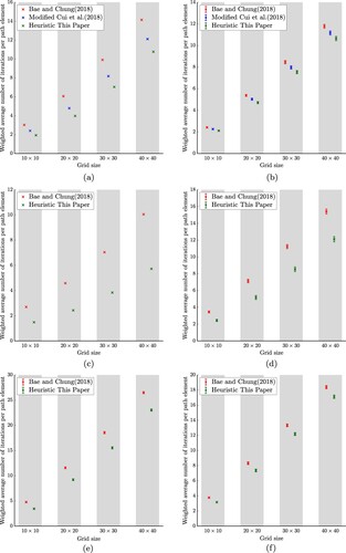
Figure 7. Average number of iterations needed to find one element of the lowest-cost path for different combinations of maximum (translation) speed and maximum rotation speed, for a $30\times 30$ rectangular grid with $0\mathrm{\%}$ of the grid elements blocked.

3D plot showing the metric (i.e. the weighted average number of iterations per path element) for different speeds and rotation speeds and for (in descending order of the sample mean for each combination of speeds) control strategies of Bae and Chung (), modified Cui et al. (), and Heuristic This Paper. There is no overlap in 3D plots between different control strategies.

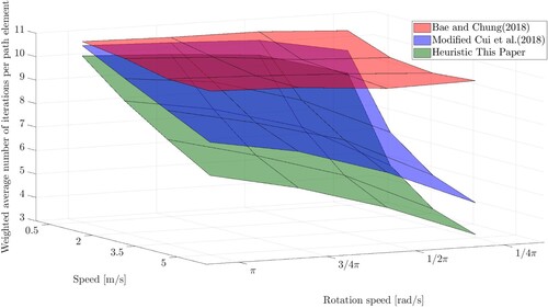
Table B1. Symbols and their meaning in Algorithms 1–3.

Symbol	Meaning
E	Set of all edges in graph $G=(V,E)$
$v_s$	Source vertex
$v_d$	Destination vertex
$p_{\mathrm{t}\mathrm{u}\mathrm{r}\mathrm{n}}$	Turning costs per radian
c	Set of all edge weights $c_{v_i{v}_j}$ for all edges E
$s_{max}$	Maximum AGV speed
${\mathrm{\Phi }}_{\mathrm{s}\mathrm{t}\mathrm{a}\mathrm{r}\mathrm{t}}$	Start orientation
${\mathrm{\Phi }}_{\mathrm{e}\mathrm{n}\mathrm{d}}$	End orientation
$P_{v_s,v_d}$	Lowest-cost path from source vertex $v_s$ to destination vertex $v_d$
$v_x.g$	Actual costs (found so far) from source vertex $v_s$ to vertex $v_x$ (i.e. value for $g(v_s,v_x)$)
$v_x.h$	Estimated costs (found so far) from vertex $v_x$ to destination vertex $v_d$ (i.e. value for $h(v_x,v_d)$)
$v_x.f$	Lowest value for actual costs plus estimated costs found so far, from source vertex $v_s$ to destination vertex $v_d$ via vertex $v_x$ (i.e. value for $f(v_s,v_x,v_d)$)
$v_x.\mathrm{p}\mathrm{r}\mathrm{e}\mathrm{d}$	Predecessor of vertex $v_x$ in lowest-cost path (found so far)
$L_{\mathrm{o}\mathrm{p}\mathrm{e}\mathrm{n}}$	Set with all open vertices (i.e. vertices to expand)
$L_{\mathrm{c}\mathrm{l}\mathrm{o}\mathrm{s}\mathrm{e}\mathrm{d}}$	Set with all closed vertices (i.e. vertices that have been expanded)
$v_c$	Current vertex
$v_{\mathrm{s}\mathrm{u}\mathrm{c}\mathrm{c}}$	Successor vertex
$g^{\prime }$	Actual costs (found so far) from source vertex $v_s$ to vertex $v_{\mathrm{s}\mathrm{u}\mathrm{c}\mathrm{c}}$ (with current vertex $v_c$ as predecessor)
$h^{\prime }$	Estimated costs from vertex $v_{\mathrm{s}\mathrm{u}\mathrm{c}\mathrm{c}}$ (with current vertex $v_c$ as predecessor) to destination vertex $v_d$
$f^{\prime }$	Value for actual costs (found so far) plus estimated costs, from source vertex $v_s$ to destination vertex $v_d$ via vertex $v_{\mathrm{s}\mathrm{u}\mathrm{c}\mathrm{c}}$ (with current vertex $v_c$ as predecessor)
$\left|\theta \right|$	Minimum absolute angle of rotation
${\mathrm{\Phi }}_{(v_x,v_y})$	Orientation of edge $(v_x,v_y)\in E$
$\left|d\right(v_e,v_d\left)\right|$	Magnitude of the Euclidean vector $d(v_e,v_d)$ directed from vertex $v_e$ to destination vertex $v_d$

Figure A1. Minimum absolute angles of rotation $\left|{\theta }_1\right|$, $\left|{\theta }_2\right|$, $\left|{\theta }_4\right|$, $\left|{\theta }_5\right|$, and $\left|{\theta }_6\right|$. (a) $\left|{\theta }_1\right|>\left|{\theta }_5\right|$ and (b) $\left|{\theta }_1\right|<\left|{\theta }_5\right|$.

(a) Vertices (with, respectively, orientations and ), , and are drawn in such a way that the minimum angles of rotation , and are all in counterclockwise direction, and such that . (b) Vertices (with, respectively, orientations and ), , and are drawn in such a way that the minimum angles of rotation and are in counterclockwise direction, and and are in clockwise direction, and such that .

Bae, J., and W. Chung. 2018. “A Heuristic for Path Planning of Multiple Heterogeneous Automated Guided Vehicles.” International Journal of Precision Engineering and Manufacturing 19 (12): 1765–1771.

 Web of Science ®Google Scholar

Bae, J., and W. Chung. 2019. “Efficient Path Planning for Multiple Transportation Robots Under Various Loading Conditions.” International Journal of Advanced Robotic Systems 16 (2): 1–9.

 Web of Science ®Google Scholar

Ballamajalu, R., M. Li, F. Sahin, C. Hochgraf, R. Ptucha, and M. E. Kuhl. 2020, August 20-21. “Turn and Orientation Sensitive A ∗ for Autonomous Vehicles in Intelligent Material Handling Systems.” IEEE International Conference on Automation Science and Engineering, 606–611.

 Google Scholar

Chaudhari, A. M., M. R. Apsangi, and A. B. Kudale. 2017, March 24-25. “Improved A-Star Algorithm with Least Turn for Robotic Rescue Operations.” Communications in Computer and Information Science 776: 614–627.

 Google Scholar

Cui, Y., D. P. Ma, Y. Fang, and Z. Lei. 2018. “Conflict-Free Path Planning of AGV Based on Improved A-star Algorithm.” 2nd International Conference on Information, Communication and Engineering (ICICE 2018), Hangzhou, Zhejiang Province, P.R. China, November 9-13, 31–34.

 Google Scholar

Jia, F., C. Ren, Y. Chen, and Z. Xu. 2017. “A System Control Strategy of a Conflict-Free Multi-AGV Routing on Improved A ∗ Algorithm.” 2017 24th International Conference on Mechatronics and Machine Vision in Practice (M2VIP), Auckland, New Zealand, November 21–23, 1–6.

 Google Scholar

Lian, Y., and W. Xie. 2019. “Improved A ∗ Multi-AGV Path Planning Algorithm Based on Grid-Shaped Network.” 2019 Chinese Control Conference (CCC), Guangzhou, China, July 27–30, 2088–2092.

 Google Scholar

Lian, Y., W. Xie, and L. Zhang. 2020, July 11-17. “A Probabilistic Time-Constrained Based Heuristic Path Planning Algorithm in Warehouse Multi-AGV Systems.” IFAC-PapersOnLine, Vol. 53, 2538–2543.

 Google Scholar

Lin, M., K. Yuan, C. Shi, and Y. Wang. 2017. “Path Planning of Mobile Robot Based on Improved A ∗ Algorithm.” 2017 29th Chinese Control and Decision Conference (CCDC), Chongqing, China, May 28–30, 3570–3576.

 Google Scholar

Liu, Y., M. Chen, and H. Huang. 2019. “Multi-Agent Pathfinding Based on Improved Cooperative A ∗ in Kiva System.” 2019 5th International Conference on Control, Automation and Robotics (ICCAR), Beijing, China, April 19–22 633–638.

 Google Scholar

Liu, X., and D. Gong. 2011. “A Comparative Study of A-Star Algorithms for Search and Rescue in Perfect Maze.” 2011 International Conference on Electric Information and Control Engineering, Wuhan, China, March 25-27, 24–27.

 Google Scholar

Mu, T., J. Zhu, X. Li, and J. Li. 2020, November 22-25. “Research on Two-Stage Path Planning Algorithms for Storage Multi-AGV.” Communications in Computer and Information Science 1160: 418–430.

 Google Scholar

Shi, J., Y. Su, C. Bu, and X. Fan. 2020. “A Mobile Robot Path Planning Algorithm Based on Improved A*.” Journal of Physics: Conference Series 1486: 032018.

 Google Scholar

Wang, C., L. Wang, J. Qin, Z. Wu, L. Duan, Z. Li, M. Cao, et al. 2015. “Path Planning of Automated Guided Vehicles Based on Improved A-Star Algorithm.” 2015 IEEE International Conference on Information and Automation, Lijiang, Yunnan, China, August 8-10, 2071–2076.

 Google Scholar

Wang, Z., and X. Xiang. 2018. “Improved Astar Algorithm for Path Planning of Marine Robot.” 2018 37th Chinese Control Conference (CCC), Wuhan, China, July 25-27, 5410–5414.

 Google Scholar

Zheng, T., Y. Xu, and D. Zheng. 2019. “AGV Path Planning Based on Improved A-Star Algorithm.” 2019 IEEE 3rd Advanced Information Management, Communicates, Electronic and Automation Control Conference (IMCEC), Chongqing, China, October 11-13, 1534–1538.

 Google Scholar

Data availability statement

The data that support the findings of this study are available from the corresponding author upon reasonable request.