Few-shot learning for defect detection in manufacturing

Figures & data

Figure 1. Sample from the Philips Consumer Lifestyle BV shavers dataset.

Three images showing samples of logos printed on shavers. The three examples correspond to the Philips Consumer Lifestyle BV shavers dataset's good, double print, and interrupted print cases.

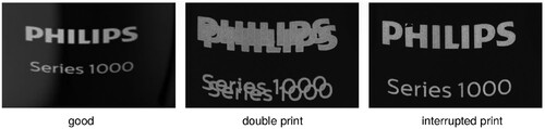
Figure 2. Sample from the Philips Consumer Lifestyle BV deco cap dataset.

Three images showing a well-manufactured product and two defective ones. The three examples correspond to good, flow-lines, and marks cases from the Philips Consumer Lifestyle BV deco cap dataset.

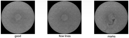
Figure 3. Sample from the Philips Consumer Lifestyle BV shaft dataset.

Four images showing a well-manufactured product and three defective ones (big dents, small dents, and stripes). The examples correspond to cases from the Philips Consumer Lifestyle BV shaft dataset.

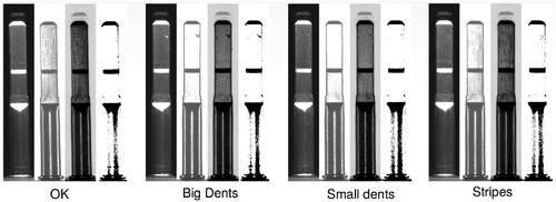
Table 1. Datasets description, describing label types and the number of data instances per label for each dataset.

Dataset	Class	Number of examples
Deco cap	good	203
	flowlines	198
	marks	191
Shaft	good	528
	big dents	2616
	small dents	954
	stripes	151
Shavers	good	2676
	double printing	244
	interrupted printing	598
IBER	good	2114
	failure 1	39
	failure 2	4
	failure 3	9

Table 2. Brief description of experiments performed: their aim, method utilised, and relevant metrics.

Experiment	Aim	Method	Metrics
1	Compare the performance of few-shot learning approaches applied to our use cases.	see Table 3	AUC ROC
2	Understand whether using DRAEM anomaly maps results in better performance of the few-shot learning approaches.	see Table 3	AUC ROC
3	Understand how data impurity affects DRAEM and how the resulting anomaly maps impact performance.	Training DRAEM model on dataset with different impurity levels and measuring the performance change of ViT backbone pre-trained with DINO and no meta-training as few-shot model.	AUC ROC
4	Compare active learning techniques used for selecting the support set in few-shot learning and determine how they impact few-shot performance	Selecting the support set using different active learning strategies and compare the performance change of the ViT backbone pre-trained with DINO and no meta-training.	AUC ROC

Table 3. Description of machine learning models used across the experiments.

Backbone	Pre train	Meta train	Type	Head
Resnet-50	cross-entropy	–	few-shot	ProtoNet
	DINO	–	few-shot	ProtoNet
ViT	cross-entropy	–	few-shot	ProtoNet
	DINO	–	few-shot	ProtoNet
		Meta-Dataset	few-shot	ProtoNet
	cross-entropy	MVTec-Capsule	few-shot	ProtoNet
Siamese	cross-entropy	MVTec-Capsule	few-shot	ProtoNet
Resnet18+MLP	cross-entropy	-	supervised	MLP

Table 4. Dataset composition for different degrees of imbalance. The rate describes the number of defective samples we consider w.r.t. the original dataset.

	Class (count)
DATASET	DECO CAP			SHAFT				SHAVERS
Rate	Good	Flowlines	Marks	Good	Big	Small	Stripe	Good	Double	Interrupted
0.00	183	0	0	476	0	0	0	2409	0	0
0.01	183	2	2	476	24	9	2	2409	3	6
0.02	183	4	4	476	48	18	3	2409	5	11
0.05	183	9	9	476	118	43	7	2409	11	27
0.10	183	18	18	476	236	86	14	2409	22	54
0.20	183	36	35	476	471	172	28	2409	44	108
0.50	183	90	86	476	1178	430	68	2409	110	270

Table 5. AUC ROC measured for classified images in a binary classification setting (defective vs. non-defective) for one-shot learning. The best results for each input type are bolded, and the second-best results are highlighted in italics. We report the 95% confidence intervals.

	MODEL			N = 1
INPUT FEATURES	Backbone	Pre train	Meta train	Deco cap	Shaft	Shavers	IBER
IMAGE	Resnet50	ImageNet	–	0.6976 ± 0.0254	0.5741 ± 0.0145	0.6589 ± 0.0235	0.9998 ± 0.0009
		DINO	–	0.5376 ± 0.0157	0.5040 ± 0.0048	0.5194 ± 0.0092	0.7626 ± 0.0334
	ViT	ImageNet	–	0.6886 ± 0.0290	0.5102 ± 0.0925	0.5668 ± 0.0206	0.9995 ± 0.0004
		DINO	–	1.0000 ± 0.0000	0.7009 ± 0.0582	0.7749 ± 0.0371	0.9995 ± 0.0003
			Meta-Dataset	0.9943 ± 0.0106	0.6339 ± 0.0796	0.7691 ± 0.0477	0.9978 ± 0.0016
		Imagenet	MVTec-Capsule	0.9999 ± 0.0001	0.5656 ± 0.0210	0.7578 ± 0.0744	0.9999 ± 0.0001
	Siamese	ImageNet	MVTec-Capsule	0.7031 ± 0.0295	0.6204 ± 0.0186	0.6429 ± 0.0227	0.9999 ± 0.0002
	Resnet18 + MLP	ImageNet	–	0.9242 ± 0.0195	0.6082 ± 0.0403	0.6304 ± 0.0497	0.9950 ± 0.0034

Table 6. AUC ROC measured for classified images in a binary classification setting (defective vs. non-defective) for five-shot learning. The best results for each input type are bolded, and the second-best results are highlighted in italics. We report the 95% confidence intervals.

	MODEL			N = 5
INPUT FEATURES	Backbone	Pre train	Meta train	Deco cap	Shaft	Shavers
IMAGE	Resnet50	ImageNet	–	0.8912 ± 0.0130	0.6657 ± 0.0125	0.7868 ± 0.0131
		DINO	–	0.5478 ± 0.0131	0.5450 ± 0.0167	0.5349 ± 0.0053
	ViT	ImageNet	–	0.8567 ± 0.0169	0.5147 ± 0.0091	0.6325 ± 0.0163
		DINO	–	0.9960 ± 0.0074	0.7596 ± 0.0305	0.8075 ± 0.0340
			Meta-Dataset	0.9971 ± 0.0033	0.7228 ± 0.0498	0.7859 ± 0.0382
		Imagenet	MVTec-Capsule	0.9986 ± 0.0023	0.5775 ± 0.0349	0.7815 ± 0.0400
	Siamese	ImageNet	MVTec-Capsule	0.8874 ± 0.0151	0.7454 ± 0.0122	0.7368 ± 0.0148
	Resnet18 + MLP	ImageNet	–	0.9803 ± 0.0045	0.7282 ± 0.0217	0.7317 ± 0.0587

Table 7. AUC ROC (one vs. rest) measured for classified images in a multiclass classification setting for one-shot learning. The best results for each input type are bolded, and the second-best results are highlighted in italics. We report the 95% confidence intervals.

	MODEL			N = 1
INPUT FEATURES	Backbone	Pre train	Meta train	Deco cap	Shaft	Shavers	IBER
IMAGE	Resnet50	ImageNet	–	0.7942 ± 0.0193	0.5749 ± 0.0143	0.7068 ± 0.0181	0.9956 ± 0.0027
		DINO	–	0.5478 ± 0.0101	0.5049 ± 0.0021	0.5195 ± 0.0075	0.7594 ± 0.0331
	ViT	ImageNet	–	0.8002 ± 0.0222	0.5092 ± 0.0076	0.5911 ± 0.0196	0.9820 ± 0.0080
		DINO	–	0.9757 ± 0.0113	0.5788 ± 0.0486	0.7317 ± 0.0287	0.9989 ± 0.0005
			Meta-Dataset	0.9585 ± 0.0105	0.5660 ± 0.0465	0.7308 ± 0.0565	0.9977 ± 0.0017
		Imagenet	MVTec-Capsule	0.9723 ± 0.0084	0.5419 ± 0.0191	0.7241 ± 0.0608	0.9994 ± 0.0003
	Siamese	ImageNet	MVTec-Capsule	0.7956 ± 0.0221	0.6244 ± 0.0168	0.6986 ± 0.0167	0.9990 ± 0.0005
	Resnet18 + MLP	ImageNet	–	0.9587 ± 0.0116	0.5925 ± 0.0213	0.6441 ± 0.0465	0.9949 ± 0.0033

Table 8. AUC ROC (one vs. rest) measured for classified images in a multiclass classification setting for five-shot learning. The best results for each input type are bolded, and the second-best results are highlighted in italics. We report the 95% confidence intervals.

	MODEL			N = 5
INPUT FEATURES	Backbone	Pre train	Meta train	Deco cap	Shaft	Shavers
IMAGE	Resnet50	ImageNet	–	0.9167 ± 0.0097	0.6470 ± 0.0132	0.7994 ± 0.0106
		DINO	–	0.5701 ± 0.0048	0.5300 ± 0.0092	0.5312 ± 0.0060
	ViT	ImageNet	–	0.9145 ± 0.0124	0.5075 ± 0.0076	0.6848 ± 0.0142
		DINO	–	0.9947 ± 0.0011	0.6646 ± 0.0280	0.7936 ± 0.0199
			Meta-Dataset	0.9871 ± 0.0031	0.6778 ± 0.0257	0.7538 ± 0.0371
		Imagenet	MVTec-Capsule	0.9865 ± 0.0032	0.5775 ± 0.0278	0.7268 ± 0.0248
	Siamese	ImageNet	MVTec-Capsule	0.9152 ± 0.0116	0.7129 ± 0.0131	0.7866 ± 0.0108
	Resnet18 + MLP	ImageNet	–	0.9886 ± 0.0025	0.7183 ± 0.0158	0.7373 ± 0.0547

Table 9. AUC ROC measured for models in a binary classification setting (defective vs. non-defective) for one-shot learning. The best results are bolded, and the second-best results are highlighted in italics. We report the 95% confidence intervals.

	MODEL			N = 1
INPUT FEATURES	Backbone	Pre train	Meta train	Deco cap	Shaft	Shavers	IBER
ANOMALY MAP	Resnet50	Imagenet	–	0.9543 ± 0.0195	0.5930 ± 0.0169	0.8091 ± 0.0272	0.9884 ± 0.0056
		DINO	–	0.6404 ± 0.0089	0.5056 ± 0.0025	0.5500 ± 0.0050	0.7827 ± 0.0268
	ViT	Imagenet	–	0.9894 ± 0.0047	0.5520 ± 0.0136	0.6974 ± 0.0248	1.0000 ± 0.0000
		DINO	–	0.9995 ± 0.0008	0.6328 ± 0.0467	0.8261 ± 0.0613	1.0000 ± 0.0000
			Meta-Dataset	0.9999 ± 0.0001	0.6707 ± 0.0709	0.7549 ± 0.0827	1.0000 ± 0.0000
		ImageNet	MVTec-Capsule	0.9884 ± 0.0075	0.6395 ± 0.0754	0.7624 ± 0.0753	0.9991 ± 0.0009
	Siamese	ImageNet	MVTec-Capsule	0.9559 ± 0.0131	0.5603 ± 0.0158	0.6392 ± 0.0191	1.0000 ± 0.0000
	Resnet18 + MLP	ImageNet	–	0.9999 ± 0.0002	0.6424 ± 0.0473	0.7712 ± 0.1011	0.9989 ± 0.0010
IMAGE + ANOMALY MAP	Resnet50	Imagenet	–	0.6195 ± 0.0189	0.5303 ± 0.0097	0.5984 ± 0.0174	0.6662 ± 0.0192
		DINO	–	0.8623 ± 0.0420	0.5119 ± 0.0079	0.5908 ± 0.0148	0.9732 ± 0.0096
	ViT	Imagenet	–	0.5686 ± 0.0157	0.5080 ± 0.0072	0.5590 ± 0.0137	0.6993 ± 0.0180
		DINO	–	0.9998 ± 0.0003	0.6916 ± 0.0645	0.8417 ± 0.0569	1.0000 ± 0.0000
			Meta-Dataset	0.9999 ± 0.0002	0.6888 ± 0.0623	0.8033 ± 0.0173	1.0000 ± 0.0000
		ImageNet	MVTec-Capsule	0.9924 ± 0.0064	0.6382 ± 0.0603	0.7756 ± 0.0699	1.0000 ± 0.0000
	Siamese	ImageNet	MVTec-Capsule	0.6488 ± 0.0182	0.5494 ± 0.0107	0.5477 ± 0.0096	0.6441 ± 0.0211
	Resnet18 + MLP	ImageNet	–	0.9994 ± 0.0011	0.6628 ± 0.0339	0.7544 ± 0.0979	0.9999 ± 0.0001

Table 10. AUC ROC measured for models in a binary classification setting (defective vs. non-defective) for five-shot learning. The best results are bolded, and the second-best results are highlighted in italics. We report the 95% confidence intervals.

	MODEL			N = 5
INPUT FEATURES	Backbone	Pre train	Meta train	Deco cap	Shaft	Shavers
ANOMALY MAP	Resnet50	Imagenet	–	0.9918 ± 0.0017	0.6925 ± 0.0131	0.9096 ± 0.0087
		DINO	–a	0.6657 ± 0.0101	0.5132 ± 0.0029	0.5616 ± 0.0053
	ViT	Imagenet	–	0.9996 ± 0.0004	0.6207 ± 0.0128	0.8204 ± 0.0118
		DINO	–	1.0000 ± 0.0000	0.7232 ± 0.0277	0.9452 ± 0.0238
			Meta-Dataset	1.0000 ± 0.0000	0.7661 ± 0.0451	0.8851 ± 0.0238
		ImageNet	MVTec-Capsule	0.9966 ± 0.0025	0.7771 ± 0.0209	0.9019 ± 0.0457
	Siamese	ImageNet	MVTec-Capsule	0.9944 ± 0.0015	0.6341 ± 0.0132	0.7388 ± 0.0180
	Resnet18 + MLP	ImageNet	–	1.0000 ± 0.0000	0.7459 ± 0.0202	0.8947 ± 0.0301
IMAGE + ANOMALY MAP	Resnet50	Imagenet	–	0.6393 ± 0.0156	0.5519 ± 0.0093	0.6575 ± 0.0145
		DINO	–	0.9149 ± 0.0146	0.5508 ± 0.0209	0.6442 ± 0.0086
	ViT	Imagenet	–	0.5888 ± 0.0187	0.5158 ± 0.0065	0.6107 ± 0.0122
		DINO	–	1.0000 ± 0.0000	0.7871 ± 0.0245	0.9568 ± 0.0200
			Meta-Dataset	1.0000 ± 0.0000	0.7975 ± 0.0228	0.8974 ± 0.0242
		ImageNet	MVTec-Capsule	0.9992 ± 0.0006	0.7419 ± 0.0289	0.9098 ± 0.0412
	Siamese	ImageNet	MVTec-Capsule	0.6977 ± 0.0179	0.5653 ± 0.0094	0.5597 ± 0.0089
	Resnet18 + MLP	ImageNet	–	0.9999 ± 0.0001	0.7912 ± 0.0202	0.8960 ± 0.0275

Table 11. AUC ROC (one-vs-rest) measured for models in a multiclass classification setting for one-shot learning. The best results are bolded, and the second-best results are highlighted in italics. We report the 95% confidence intervals.

	MODEL			N = 1
INPUT FEATURES	Backbone	Pre train	Meta train	Deco cap	Shaft	Shavers	IBER
ANOMALY MAP	Resnet50	Imagenet	–	0.9749 ± 0.0131	0.5998 ± 0.0161	0.8427 ± 0.0243	0.9907 ± 0.0062
		DINO	–	0.6564 ± 0.0083	0.5041 ± 0.0017	0.5436 ± 0.0041	0.7804 ± 0.0271
	ViT	Imagenet	–	0.9301 ± 0.0120	0.5549 ± 0.0119	0.7054 ± 0.0226	0.9980 ± 0.0008
		DINO	–	0.9938 ± 0.0030	0.5364 ± 0.0374	0.8087 ± 0.0600	0.9999 ± 0.0001
			Meta-Dataset	0.9939 ± 0.0025	0.5552 ± 0.0320	0.7467 ± 0.0778	0.9997 ± 0.0002
		ImageNet	MVTec-Capsule	0.9764 ± 0.0082	0.5495 ± 0.0255	0.7529 ± 0.0733	0.9988 ± 0.0010
	Siamese	ImageNet	MVTec-Capsule	0.9686 ± 0.0150	0.5811 ± 0.0159	0.6975 ± 0.0196	0.9908 ± 0.0084
	Resnet18 + MLP	ImageNet	–	0.9931 ± 0.0037	0.5669 ± 0.0191	0.7651 ± 0.0939	0.9989 ± 0.0010
IMAGE + ANOMALY MAP	Resnet50	Imagenet	–	0.6430 ± 0.0193	0.5333 ± 0.0072	0.6006 ± 0.0159	0.7888 ± 0.0223
		DINO	–	0.8694 ± 0.0303	0.5129 ± 0.0048	0.5849 ± 0.0124	0.9710 ± 0.0094
	ViT	Imagenet	–	0.5639 ± 0.0195	0.5208 ± 0.0054	0.5592 ± 0.0135	0.8181 ± 0.0222
		DINO	–	0.9962 ± 0.0024	0.5711 ± 0.0475	0.8219 ± 0.0540	1.0000 ± 0.0000
			Meta-Dataset	0.9970 ± 0.0019	0.5776 ± 0.0413	0.7637 ± 0.0715	1.0000 ± 0.0000
		ImageNet	MVTec-Capsule	0.9838 ± 0.0072	0.5559 ± 0.0233	0.7628 ± 0.0677	0.9991 ± 0.0006
	Siamese	ImageNet	MVTec-Capsule	0.6469 ± 0.0208	0.5441 ± 0.0082	0.5497 ± 0.0093	0.7356 ± 0.0263
	Resnet18 + MLP	ImageNet	–	0.9944 ± 0.0034	0.5751 ± 0.0164	0.7580 ± 0.0913	0.9998 ± 0.0001

Table 12. AUC ROC (one-vs-rest) measured for models in a multiclass classification setting for five-shot learning. The best results are bolded, and the second-best results are highlighted in italics. We report the 95% confidence intervals.

	MODEL			N = 5
INPUT FEATURES	Backbone	Pre train	Meta train	Deco cap	Shaft	Shavers
ANOMALY MAP	Resnet50	Imagenet	–	0.9923 ± 0.0001	0.6988 ± 0.0117	0.9381 ± 0.0070
		DINO	–	0.6815 ± 0.0062	0.5070 ± 0.0023	0.5513 ± 0.0046
	ViT	Imagenet	–	0.9894 ± 0.0024	0.6044 ± 0.0110	0.8698 ± 0.0091
		DINO	–	0.9941 ± 0.0027	0.6013 ± 0.0122	0.9243 ± 0.0259
			Meta-Dataset	0.9954 ± 0.0023	0.6310 ± 0.0155	0.8710 ± 0.0210
		ImageNet	MVTec-Capsule	0.9810 ± 0.0073	0.6299 ± 0.0165	0.8907 ± 0.0438
	Siamese	ImageNet	MVTec-Capsule	0.9958 ± 0.0012	0.6767 ± 0.0126	0.8038 ± 0.0161
	Resnet18 + MLP	ImageNet	–	0.9941 ± 0.0028	0.6601 ± 0.0295	0.8821 ± 0.0295
IMAGE + ANOMALY MAP	Resnet50	Imagenet	–	0.6522 ± 0.0184	0.5649 ± 0.0070	0.6688 ± 0.0150
		DINO	–	0.8969 ± 0.0132	0.5454 ± 0.0129	0.6341 ± 0.0084
	ViT	Imagenet	–	0.5806 ± 0.0183	0.5331 ± 0.0057	0.6349 ± 0.0126
		DINO	–	0.9962 ± 0.0020	0.6658 ± 0.0214	0.9337 ± 0.0224
			Meta-Dataset	0.9981 ± 0.0012	0.6977 ± 0.0178	0.8844 ± 0.0206
		ImageNet	MVTec-Capsule	0.9868 ± 0.0054	0.6350 ± 0.0218	0.8962 ± 0.0403
	Siamese	ImageNet	MVTec-Capsule	0.6600 ± 0.0173	0.5655 ± 0.0076	0.5812 ± 0.0095
	Resnet18 + MLP	ImageNet	–	0.9950 ± 0.0026	0.6501 ± 0.0191	0.8924 ± 0.0266

Table 13. AUC ROC measured for multiclass classification, considering DRAEM anomaly maps as inputs. The anomaly maps are obtained from a DRAEM model trained with all available images. We specify different degrees of artificial imbalance on top of the given one (mix rate). The exact composition of the datasets for each mix rate is described in Table 4. We report the 95% confidence intervals. The models using anomaly map features are bolded when performing better than those trained solely on images.

	MODEL
INPUT FEATURES	Backbone	Pre train	Meta train	Mix rate	Deco cap	Shaft	Shavers
IMAGE	ViT	DINO	–	1.00	0.9947 ± 0.0011	0.6646 ± 0.0280	0.7936 ± 0.0199
ANOMALY MAP	ViT	DINO	–	0.00	0.9941 ± 0.0027	0.6013 ± 0.0122	0.9243 ± 0.0259
				0.01	0.9811 ± 0.0079	0.5726 ± 0.0242	0.9213 ± 0.0211
				0.02	0.9408 ± 0.0122	0.5487 ± 0.0187	0.9111 ± 0.0250
				0.05	0.8815 ± 0.0062	0.5213 ± 0.0019	0.9057 ± 0.0159
				0.10	0.7515 ± 0.0293	0.5018 ± 0.0007	0.8570 ± 0.0159
				0.20	0.6004 ± 0.0018	0.5010 ± 0.0015	0.6413 ± 0.0211
				0.50	0.5102 ± 0.0023	0.5000 ± 0.0001	0.5020 ± 0.0391

Figure 4. Plots showing AUC ROC performance based on sampling iterations for six active learning techniques and three datasets. The following naming conventions are used for the series: random (random sampling), margin (margin sampling), uncertain (uncertainty sampling), emb_resnet (EMB_ResNet-50), emb_pmf (EMB_PMF), and GradCAM (EMB_GradCAM).

Three plots showing AUC ROC performance based on sampling iterations for six active learning techniques and three datasets. The six active learning techniques considered are random sampling, margin sampling, uncertainty sampling, EMB ResNet-50, EMB PMF, and EMB GradCAM. The three datasets considered are shavers, deco cap, and shaft.

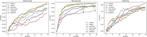
Table 14. AUC ROC measured for models in a multiclass classification setting. The best results are bolded, and the second-best results are highlighted in italics. We report the 95% confidence intervals.

		Number of sampled images
Dataset	Active learning strategy	1	5	10	20
DECO CAP	Random sampling	0.9437 ± 0.0252	0.9643 ± 0.0135	0.9811 ± 0.0052	0.9912 ± 0.0029
	Uncertainty sampling	0.9506 ± 0.0226	0.9880 ± 0.0026	0.9959 ± 0.0011	0.9994 ± 0.0002
	Margin sampling	0.9533 ± 0.0230	0.9889 ± 0.0031	0.9969 ± 0.0008	0.9708 ± 0.0375
	EMBResNet-50	0.9467 ± 0.0301	0.9690 ± 0.0067	0.9735 ± 0.0054	0.9881 ± 0.0027
	EMBPMF	0.9485 ± 0.0300	0.9762 ± 0.0052	0.9761 ± 0.0050	0.9786 ± 0.0042
	EMBGradCAM	0.9455 ± 0.0469	0.9790 ± 0.0088	0.9883 ± 0.0052	0.9934 ± 0.0032
SHAFT	Random sampling	0.6210 ± 0.0667	0.6427 ± 0.0686	0.7320 ± 0.0637	0.7612 ± 0.0212
	Uncertainty sampling	0.6266 ± 0.0686	0.6978 ± 0.0326	0.7038 ± 0.0164	0.7624 ± 0.0239
	Margin sampling	0.6023 ± 0.0747	0.6833 ± 0.0216	0.6838 ± 0.0518	0.7406 ± 0.0363
	EMBResNet-50	0.5965 ± 0.0663	0.6435 ± 0.0442	0.6889 ± 0.0170	0.7870 ± 0.0194
	EMBPMF	0.6099 ± 0.0333	0.6866 ± 0.0444	0.7154 ± 0.0664	0.7667 ± 0.0492
	EMBGradCAM	0.6075 ± 0.0525	0.6573 ± 0.0354	0.7014 ± 0.0326	0.7519 ± 0.0239
SHAVERS	Random sampling	0.6987 ± 0.0312	0.7206 ± 0.0289	0.7582 ± 0.0299	0.7934 ± 0.0251
	Uncertainty sampling	0.6541 ± 0.0303	0.7271 ± 0.0236	0.7679 ± 0.0187	0.7979 ± 0.0169
	Margin sampling	0.6687 ± 0.0256	0.7226 ± 0.0346	0.7519 ± 0.0293	0.8129 ± 0.0199
	EMBResNet-50	0.6601 ± 0.0332	0.6621 ± 0.0312	0.6865 ± 0.0252	0.7205 ± 0.0385
	EMBPMF	0.6664 ± 0.0323	0.7072 ± 0.0218	0.7371 ± 0.0199	0.7813 ± 0.0237
	EMBGradCAM	0.6748 ± 0.0390	0.7078 ± 0.0447	0.7023 ± 0.0375	0.7508 ± 0.0556

Table 15. Comparison of best models, considering Image (I) and Image+Heatmap (I+H) input features. The results were taken from Table 5 and Table 6 regarding the binary classification case.

		MODEL			DATASET
N	INPUT FEATURES	Backbone	Pre train	Meta train	Deco cap	Shaft	Shavers	IBER
1	I	ViT	DINO	–	1.0000 ± 0.0000	0.7009 ± 0.0582	0.7749 ± 0.0371	0.9995 ± 0.0003
				Meta-Dataset	0.9943 ± 0.0106	0.6339 ± 0.0796	0.7691 ± 0.0477	0.9978 ± 0.0016
			Imagenet	MVTec-Capsule	0.9999 ± 0.0001	0.5656 ± 0.0210	0.7578 ± 0.0744	0.9999 ± 0.0001
	I+H	ViT	DINO	–	0.9998 ± 0.0003	0.6916 ± 0.0645	0.8417 ± 0.0569	1.0000 ± 0.0000
				Meta-Dataset	0.9999 ± 0.0002	0.6888 ± 0.0623	0.8033 ± 0.0173	1.0000 ± 0.0000
			ImageNet	MVTec-Capsule	0.9924 ± 0.0064	0.6382 ± 0.0603	0.7756 ± 0.0699	1.0000 ± 0.0000
5	I	ViT	DINO	–	0.9960 ± 0.0074	0.7596 ± 0.0305	0.8075 ± 0.0340	–
				Meta-Dataset	0.9971 ± 0.0033	0.7228 ± 0.0498	0.7859 ± 0.0382	–
	I+H	ViT	DINO	–	1.0000 ± 0.0000	0.7871 ± 0.0245	0.9568 ± 0.0200	–
				Meta-Dataset	1.0000 ± 0.0000	0.7975 ± 0.0228	0.8974 ± 0.0242	–

Table 16. Comparison of best models, considering Image (I) and Image+Heatmap (I+H) input features. The results were taken from Table 7 and Table 8 regarding the multiclass classification case.

		MODEL			DATASET
N	INPUT FEATURES	Backbone	Pre train	Meta train	Deco cap	Shaft	Shavers	IBER
1	I	ViT	DINO	–	0.9757 ± 0.0113	0.5788 ± 0.0486	0.7317 ± 0.0287	0.9989 ± 0.0005
				Meta-Dataset	0.9585 ± 0.0105	0.5660 ± 0.0465	0.7308 ± 0.0565	0.9977 ± 0.0017
			Imagenet	MVTec-Capsule	0.9723 ± 0.0084	0.5419 ± 0.0191	0.7241 ± 0.0608	0.9994 ± 0.0003
		Siamese	ImageNet	MVTec-Capsule	0.7956 ± 0.0221	0.6244 ± 0.0168	0.6986 ± 0.0167	0.9990 ± 0.0005
	I+H	ViT	DINO	–	0.9962 ± 0.0024	0.5711 ± 0.0475	0.8219 ± 0.0540	1.0000 ± 0.0000
				Meta-Dataset	0.9970 ± 0.0019	0.5776 ± 0.0413	0.7637 ± 0.0715	1.0000 ± 0.0000
			ImageNet	MVTec-Capsule	0.9838 ± 0.0072	0.5559 ± 0.0233	0.7628 ± 0.0677	0.9991 ± 0.0006
		Siamese	ImageNet	MVTec-Capsule	0.6469 ± 0.0208	0.5441 ± 0.0082	0.5497 ± 0.0093	0.7356 ± 0.0263
5	I	ViT	DINO	–	0.9947 ± 0.0011	0.6646 ± 0.0280	0.7936 ± 0.0199	–
				Meta-Dataset	0.9871 ± 0.0031	0.6778 ± 0.0257	0.7538 ± 0.0371	–
		Resnet18 + MLP	ImageNet	–	0.9886 ± 0.0025	0.7183 ± 0.0158	0.7373 ± 0.0547	–
	I+H	ViT	DINO	–	0.9962 ± 0.0020	0.6658 ± 0.0214	0.9337 ± 0.0224	–
				Meta-Dataset	0.9981 ± 0.0012	0.6977 ± 0.0178	0.8844 ± 0.0206	–
		Resnet18 + MLP	ImageNet	–	0.9950 ± 0.0026	0.6501 ± 0.0191	0.8924 ± 0.0266	–

Data availability statement

The data is not available due to restrictions.