
Figures & data
Figure 1. (a) photographs of the high-throughput shear testing device with the enlarged (b) specimen holder, (c) loading part, and (d) butt joint specimen.
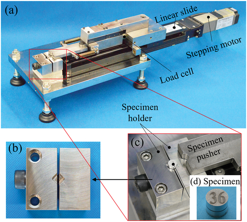
Figure 2. Stress–strain curves of Epoxy-1 and Epoxy-2.
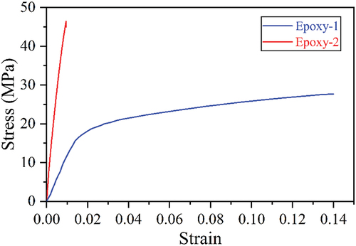
Table 1. Typical properties of two types of epoxy adhesives.
Figure 3. (a) FE model of the moisture diffusion simulation with mesh distribution. The mesh size was 0.1 mm. (b) simulation results of the normalized concentration of water in the adhesive layer.
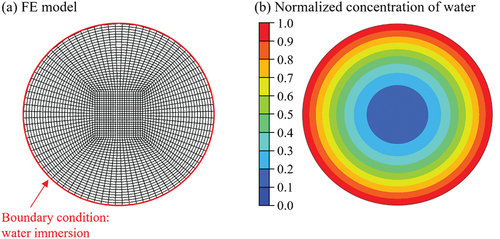
Figure 4. Overall process of high-throughput preparation of the butt shear-joint (BSJ) specimens. ① aluminum plate after pre-machining. ② 5-layered structures. ③ 5-layered structures after the final milling process. ④ removing specimens after hot water immersion. ⑤ a sample specimen.
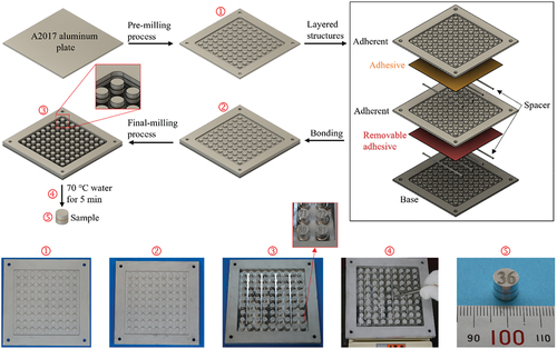
Figure 5. Distributions of (a) shear stress and (b) peeling stress at the middle surface of the adhesive layer for single-lap shear joint and butt shear joint specimens. Color bar shows the normalized shear stress and peeling stress, where τ0 = applied force/bonding area. The applied force was along the z-axis.
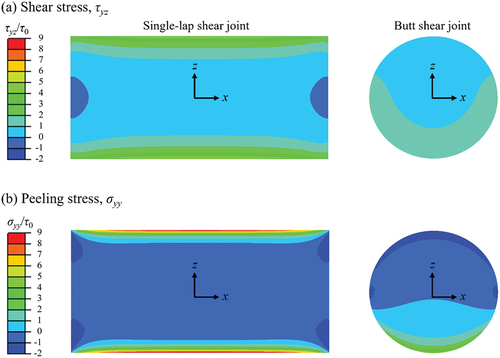
Figure 6. (a) force – displacement curves of three types of butt joint specimens. (b) illustration of the fracture behaviors of adhesive layers. (c) photographs of fracture surfaces. (d) laser microscope images of fracture surfaces. (e) epi-fluorescence microscope images of fracture surfaces.
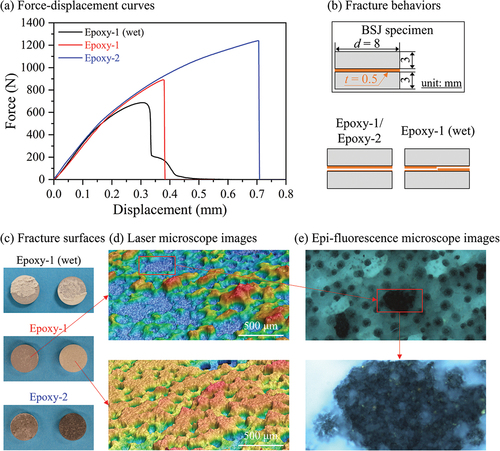
Figure 7. Averages and standard deviations of the shear strength of three types of specimens measured in high-throughput shear tests.
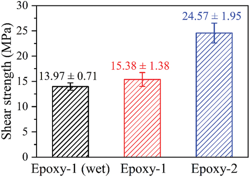
Figure 8. Histogram plots of the shear strength measurements for (a) Epoxy-1 after moisture absorption, (b) Epoxy-1, and (c) Epoxy-2. A normal distribution curve was estimated and overlaid in each graph.
Figure 9. Probability plots of shear strength measurements for (a) Epoxy-1 after moisture absorption, (b) Epoxy-1, (c) Epoxy-2, and (d) a comparison of the three types of specimens.
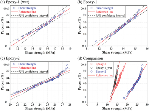
Figure 10. Quantile–quantile (Q – Q) plots for Epoxy-1 after moisture absorption. Five distributions (a) normal, (b) Lognormal, (c) exponential, (d) Weibull, and (e) Gamma were investigated to assess the goodness of fit to experimental data.
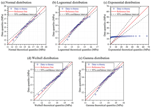
Figure 11. Q – Q plots for Epoxy-1.
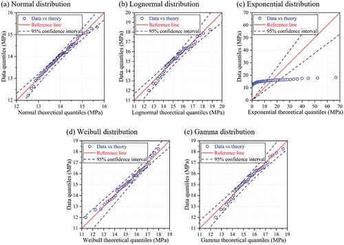
Figure 12. Q – Q plots for Epoxy-2.
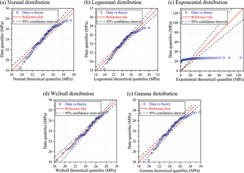
Table 2. Shape and scale factors of each specimen for various distributions.
Table 3. Chi-square test values χ2 of the data in Q–Q plots for three types of specimens and various distribution functions.
Table 4. Coefficient of determination R2 of the data in the Q–Q plots for three types of specimens and various distribution functions.
Table 5. Pearson correlation coefficient rxy of the data in the Q–Q plots for three types of specimens and various distribution functions.