Figures & data
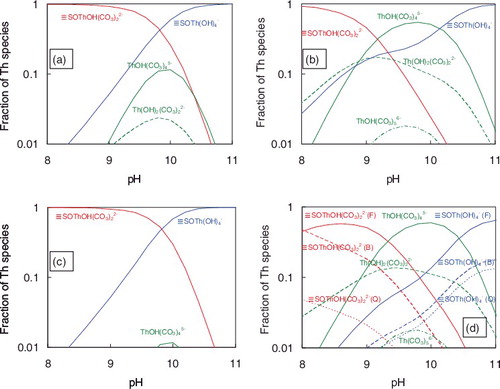
Figure 1. Solubility of Th in 0.01 mol dm−3 NaHCO3 solution (a) and 0.1 mol dm−3 NaHCO3 solution (b) calculated with existing thermodynamic data [Citation2,Citation3].
![Figure 1. Solubility of Th in 0.01 mol dm−3 NaHCO3 solution (a) and 0.1 mol dm−3 NaHCO3 solution (b) calculated with existing thermodynamic data [Citation2,Citation3].](/cms/asset/fa251835-aedc-4132-8a73-cead45d2c238/tnst_a_1138901_f0001_oc.jpg)
Figure 2. Scanning electron microscope images of the employed solids (×100 magnification).
Table 2. Experimental variables and data for Th sorption on albite.
Table 3. Experimental variables and data for Th sorption on quartz.
Table 4. Experimental variables and data for Th sorption on biotite.
Table 5. Experimental variables and data for Th sorption on granite.
Figure 3. Comparison of Kd values for Th obtained in this study and previously reported ones: (a) albite, (b) quartz [Citation12,Citation14], (c) biotite, and (d) granite [Citation11]. ‘0.01 M’ represents the 0.01 mol dm−3 NaHCO3 concentration. Previous data for albite and biotite are not available.
![Figure 3. Comparison of Kd values for Th obtained in this study and previously reported ones: (a) albite, (b) quartz [Citation12,Citation14], (c) biotite, and (d) granite [Citation11]. ‘0.01 M’ represents the 0.01 mol dm−3 NaHCO3 concentration. Previous data for albite and biotite are not available.](/cms/asset/f9c2e73c-b61f-4a4c-bc27-ed7783521b08/tnst_a_1138901_f0003_oc.jpg)
Table 6. Existing literature values of equilibrium constants for surface complexation of Th.
Figure 4. Correlation of surface complexation constants of metal species sorbing on the mineral surface with the corresponding aqueous hydrolysis constants (blue and green marks) summarized in Bradbury and Baeyens [Citation27,Citation28]. The blue line shows LFER for montmorillonite and the green dotted line for illite. Red marks are the data reported by Ervanne et al. [Citation30].
![Figure 4. Correlation of surface complexation constants of metal species sorbing on the mineral surface with the corresponding aqueous hydrolysis constants (blue and green marks) summarized in Bradbury and Baeyens [Citation27,Citation28]. The blue line shows LFER for montmorillonite and the green dotted line for illite. Red marks are the data reported by Ervanne et al. [Citation30].](/cms/asset/37cc3f16-8d2e-4cb8-b7bd-7fb5d19141c4/tnst_a_1138901_f0004_oc.jpg)
Figure 5. Comparison of Kd values of Th predicted using the NEM (lines) with experimentally measured ones (marks).
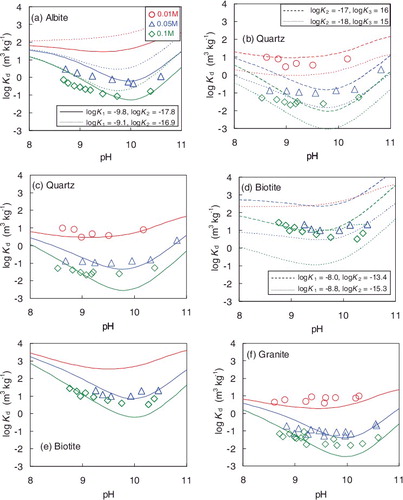
Table 7. Model parameters and equilibrium constants for the NEM calculation.
Figure 6. Calculated mole fraction of Th species under 0.05 mol dm−3 NaHCO3 condition. (a) Albite, (b) quartz, (c) biotite, (d) granite and (e) granite calculated using one order of magnitude lower K1–K7 values for feldspar. (F), feldspar; (Q), quartz; (B), biotite.