Application of Bayesian machine learning for estimation of uncertainty in forecasted plume directions by atmospheric dispersion simulations

Figures & data

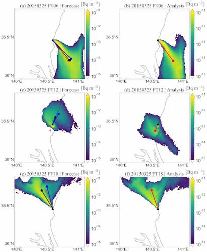
Figure 1. Computational domains for WSPEEDI-DB calculations. The colors indicate the ground height above sea level. The triangle denotes the release point, which is the location of the nuclear science research institute, JAEA.

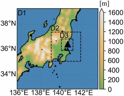
Table 1. Configuration of WRF for each domain.

Domain	D1	D2	D3
Horizontal grid points	78 × 78	88 × 88	103 × 103
Horizontal grid spacing (km)	9	3	1
Vertical layers	30
Time step (s)	36	12	4
Grid nudging	On	Off
Microphysics	Morrison microphysics [23]
Cumulus	Betts – Miller–Janjić Cumulus [24]		Off
Boundary layer	Mellor – Yamada–Nakanishi – Niino PBL Level 2.5 [25]
Surface layer	Mellor – Yamada–Nakanishi – Niino
Land surface	Five-layer thermal diffusion [21]
Shortwave radiation	Rapid radiative transfer model [26]
Longwave radiation	Dudhia [27]

Table 2. Configuration of GEARN for each domain.

Domain	D2	D3
Horizontal grid points	86 × 86	101 × 101
Horizontal grid spacing (km)	3	1
Vertical layers	28
Time step (s)	12	4
Output time interval (h)	1
Horizontal diffusion parameter	Pasquil – Gifford chart (stability: neutral)
Release point	NSRI (36.46°N, 140.60°E)
Release radionuclide	^137Cs
Release rate (Bq h^−1)	1
Release period (h)	1
Release height (m)	100
Particle number (h^−1)	10^6

Figure 2. Illustration of the analysis and forecast inputs derived from the GSM-JP dataset.

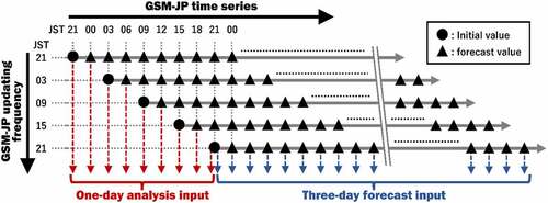
Figure 3. Configuration of the analysis and forecast outputs used in the Bayesian machine learning. FTx indicates the 6-hourly forecast periods. The data in the analysis output, which is unavailable at the time of forecast calculation in DAY0, is shown as a red dashed-line.

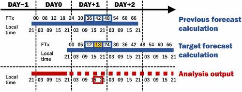
Figure 4. Schematic regarding the method for evaluating the uncertainty of the plume direction. G^m shown as a vector (black) with the release point as the origin and the rectangle area in (a) indicate the most probable point and probability distribution of the plume centroid calculated using the Bayesian machine learning, respectively. The solid and dashed green vectors in (a) and (b) are the one forming the maximum angle Φ with G^m and its line symmetrical one with respect to G^m, respectively. G^f and G^a in (b) indicate the vectors (blue and red, respectively) of the plume centroid from the forecast and analysis outputs, respectively. The predicted uncertainty of the plume direction is defined as the angle Φ_m to G^f, which is shown as a central angle with a light blue fan-shape in (c).

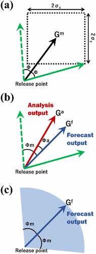
Table 3. Coefficients of determination R² for the x- and y-components of the plume centroid estimated using Bayesian machine learning. The coefficients calculated from the training and test data are shown in the table.

6-hourly forecast period	Coefficients of determination R^2
	Gx		Gy
	Training	Test	Training	Test
FT06	0.991	0.990	0.989	0.990
FT12	0.959	0.953	0.953	0.956
FT18	0.917	0.907	0.927	0.920
FT24	0.853	0.851	0.868	0.859
FT30	0.802	0.811	0.805	0.766
FT36	0.828	0.782	0.805	0.791

Figure 5. Boxplot of Φ_a (analysis) and Φ_m (model) for each FT. The top and bottom of the boxes indicate upper and lower quartiles, respectively; the horizontal bar in the box and an open circle show median and mean values, respectively; the upper and lower whiskers show the maximum and minimum angles. Respectively, except for outliers described outside the upper whisker.

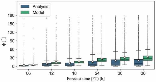
Figure 6. Time series of Φ_a (analysis) and Φ_m (model) from FT6 to FT36 on (a) May 24, (b) February 10, and (c) March 25, 2015. Black triangles and red circles indicate the angles from the analysis output and the Bayesian model, respectively.

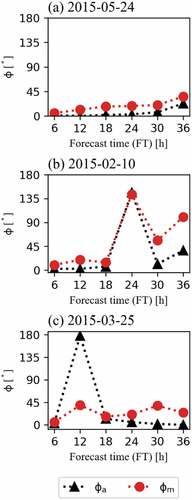
Figure 7. Heatmap showing the percentage of data contained in each domain. The horizontal and vertical axes show the values of Φ_a (analysis) and Φ_m (model), respectively. The value plotted in each domain indicates the percentage.

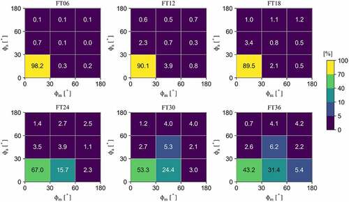
Figure 8. Schematic regarding the judgment of (a) ‘misses,’ (b) ‘hits’ for high uncertainty, (c) ‘hits’ for low uncertainty, and ‘false alert.’ the fan-shape colored as light blue indicates the uncertainty of forecasted plume direction.

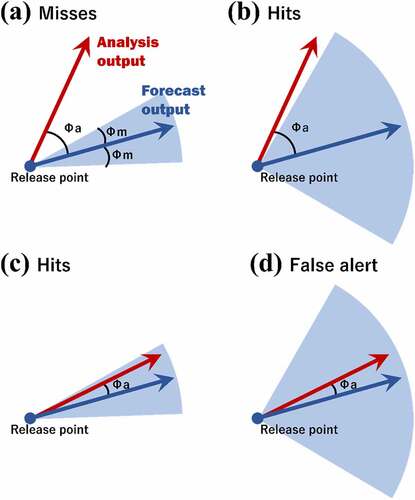
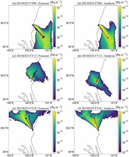
Figure 9. Horizontal distribution of ¹³⁷Cs concentration from FT06 to FT18 on March 25, 2015. The triangle symbol shows the location of the release point. The left and right columns of the figure show the results of the forecast and analysis outputs, respectively. Black and blue lines in the left column describe the vector indicating the plume centroid (shown as a filled circle at the line end) by the forecast output and the Bayesian model, respectively. The dashed red line in the left column and the red line in the right column describe the vector indicating the plume centroid by the analysis output.

Morrison H, Thompson G, Tatarskii V. Impact of cloud microphysics on the development of trailing stratiform precipitation in a simulated squall line: Comparison of one-and two-moment schemes. Mon Wea Rev. 2009;137(3):991–1007.

 Web of Science ®Google Scholar

Janjić ZI. The step-mountain eta coordinate model: Further developments of the convection, viscous sublayer, and turbulence closure schemes. Mon Wea Rev. 1994;122(5):927–945.

 Web of Science ®Google Scholar

Nakanishi M, Niino H. An improved Mellor–Yamada level-3 model with condensation physics: Its design and verification. Bound-Lay Meteorol. 2004;112(1):1–31.

 Web of Science ®Google Scholar

Skamarock WC, Klemp JB, Dudhia J, et al. A description of the advanced research WRF version 3. USA: National Center for Atmospheric Research; 2008. (NCAR/TN-475STR).

 Google Scholar

Mlawer EJ, Taubman SJ, Brown PD, et al. Radiative transfer for inhomogeneous atmospheres: RRTM, a validated correlated-k model for the longwave. J Geophys Res Atmos. 1997;102(D14):16663–16682. DOI:10.1029/97JD00237

 Web of Science ®Google Scholar

Dudhia J. Numerical study of convection observed during the winter monsoon experiment using a mesoscale two-dimensional model. J Atmos Sci. 1989;46(20):3077–3107.

 Web of Science ®Google Scholar