
Figures & data
Figure 1. (A) Location map. NIFS = North Island Fault System. (B) Wellington City street map showing gravity stations. (C) Geological map showing profile lines (labelled with letters) and boreholes either intersecting basement or over 50 m deep. Geology from Begg and Mazengarb (Citation1996), simplified geological overlay based on Kaiser et al. (Citation2019).
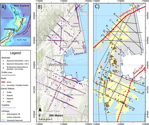
Figure 2. (A) Bouguer gravity anomaly map. Point data gridded using kriging and contoured in mGal. (B) Regional gravity field polynomial. (C) Residual gravity anomaly map. Point data gridded using kriging and contoured in mGal. The green dashed circle denotes an area showing variation in the residual anomaly over bedrock.
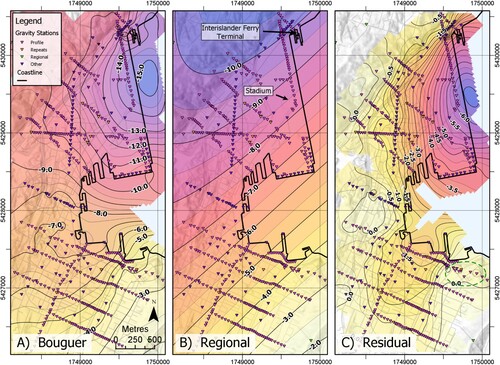
Figure 3. The effect of a DC shift and weathered greywacke on model fit. (A) Line A () geological profile with no DC shift, showing the poor fit resulting from honouring the borehole basement constraints. (B) The addition of a −0.8 mGal DC shift, which allows the model to best fit borehole constraints while maintaining smooth, realistic basement topography. This introduces a misfit to the residual anomaly on the hills adjacent to the sedimentary basin. (C) Addition of a zone of weathered greywacke with density 2.4 Mg/m3 on the hills, lowering the calculated anomaly to fit the DC – shifted anomaly.
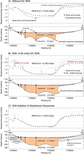
Table 1. Density data and estimations for each sediment modelling unit.
Figure 4. Line B residual anomalies and profile model. (A) Residual anomalies resulting from adoption of five different regional fields. The regionals are created by varying the weighting assigned to profile stations as compared to regional stations. The preferred regional (black) derives from a higher weighting to some profile stations and lower to some outlier stations. (B) The geological profile modelled to fit the preferred residual anomaly, with basement contact from the model fitting the ‘zero profile weighting’ regional field (green) and from the shallow and deep interpretations (blue and red) overlain. In each model, only the basement contact is adjusted, while the other layers are kept the same. Note that the depth range of the latter two models entirely encompasses the green line, and this is therefore used to define the depth uncertainty (hashed). The 1969 borehole recording a basement intersection that strongly controls the Hill et al. (Citation2020) model (grey, dashed) and does not fit the gravity model is labelled.
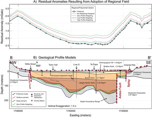
Table 2. Key parameters for each profile. Max constrained basement depth is the maximum depth directly beneath a gravity station.
Figure 5. Dip sensitivity testing on Line A. (A) Observed residual anomalies with calculated gravity for each of the three models on right. (B) Fault models show the maximum possible normal and reverse dips for the Aotea Fault which do not increase the RMS error of the fit to observations of 0.029 mGal.
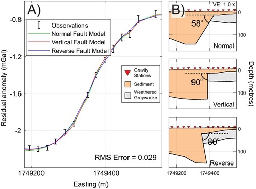
Figure 6. Profile for Line J. (A) Observed residual anomalies and calculated gravity response due to the geological model. (B) Geological model with basement contact from Hill et al. (Citation2020) for this profile in purple. Gravity stations are red triangles, and intersections with other profile lines are marked in black. There are no deep boreholes on this profile.
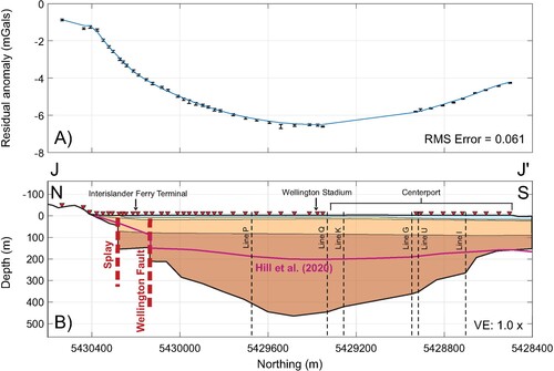
Figure 7. Preferred basin depth map produced by kriging point data extracted from profile models and contoured in metres. Profile lines labelled in grey. Fault traces located with moderate to high confidence from seismic, gravity or geologic data are solid black lines, inferred fault traces dashed black lines. The proposed extension to the Lambton Fault is in red.
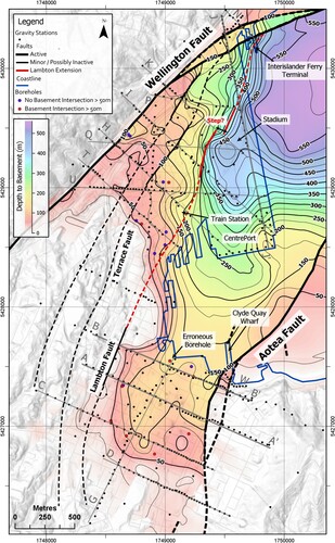
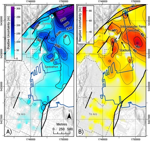
Figure 8. (A) Map of the difference between the preferred depth map and the deep interpretation, representing depth uncertainty in the positive, that is, deeper direction. (B) Map of the difference between the preferred depth map and the shallow interpretation, representing depth uncertainty in the negative, that is, shallower direction.
Data availability statement
The authors confirm that the data supporting the findings of this study are openly available in Mendeley Data at http://doi.org/10.17632/j2txy867b4.1. The data are also planned to be available from the GNS Science gravity database, accessible through the E Tūhura – Explore Zealandia portal: https://data.gns.cri.nz/tez/. Further details of methods used in this study are available from the Victoria University of Wellington library: https://doi.org/10.26686/wgtn.15176061.v1 (Stronach Citation2021).