
Figures & data
Figure 1. A, Tectonic index map of New Zealand, showing motion of the Pacific Plate relative to Australia (black arrow, from DeMets et al. Citation1994), the Alpine Fault (in red), and the location of the enlargement that is part B of this figure. B, Location of the study area (Crawford Knob, indicated by a blue dot) in the non-mylonitic Alpine Schist near Franz Josef Glacier in the central Southern Alps. The faults are part of an exhumed corridor of steeply-dipping brittle-ductile faults (after Little et al. Citation2007).
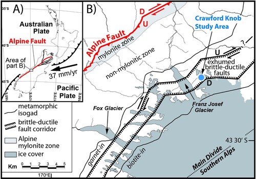
Figure 2. A, Cartoon showing the brittle-ductile fault corridor interpreted as a zone of backshearing that transiently deforms mid-crustal rocks of the Pacific Plate as they are tilted across the base of the Alpine Fault ramp (after Little Citation2004). B, Schematic block diagram (looking NNE) showing kinematics of faults in the corridor. Oblique-slip on the subparallel array of steep faults accommodates a net up-to-the-NW angular shear of the Pacific Plate (∼22°, after Wightman and Little Citation2007) as well as a subequal magnitude of dextral angular shear. The faults cut and offset the metamorphic foliation in the Alpine Schist (dashed planes) and a set of generally east-dipping quartz veins (solid blue layers). C, Schematic view of one of the quartz veins, showing the typically brittle-to-ductile nature of their offset.
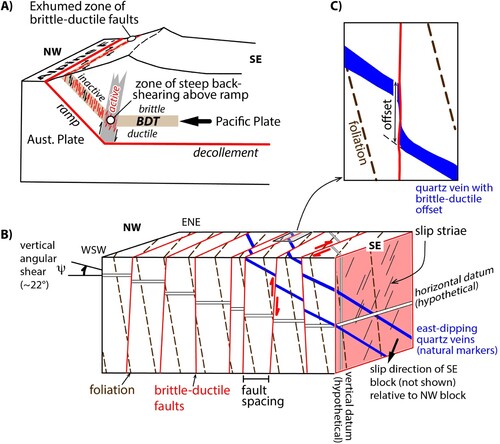
Figure 3. Outcrops of schist below Crawford Knob. A, subvertical aerial photograph from approximately 50 m above ground level showing exposed schist locally mantled by patches of gravel or alpine vegetation. Note tents from field camp on far right-hand side of the image for scale. B, Oblique view south from ground level of outcrop (view direction and position shown in A and people for scale) showing smooth, glacially sculptured outcrop surface, pelite and psammite layers in the schist (dark- and light-coloured bands, respectively), quartz veins (white masses); and brittle-ductile faults (red dashed traces). The irregular dark stain on the left-hand side of the photograph is water (also visible in panel A).
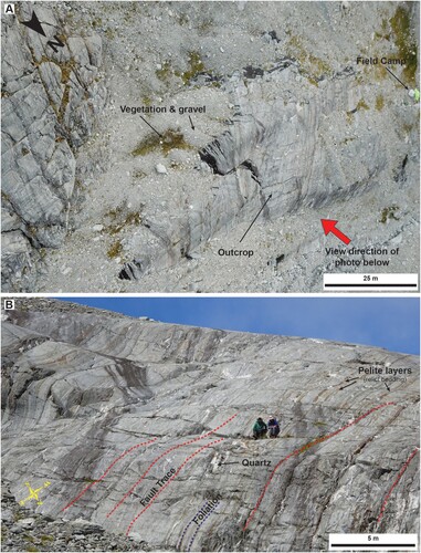
Figure 4. Outcrop exposure of faults. A, Two faults displacing a 2-3 cm-thick quartz-calcite vein. B, Wider view showing several faults that dextrally offset a thick relict bed of pelite (brown-coloured band) as well as numerous cm-thick quartz veins (white stripes). C, Example of mineral fibre lineations (red arrows) defined by quartz-calcite-chlorite vein material that infills some fault planes (fault plane dipping NNW, lineation plunging ∼30o SW).
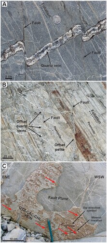
Figure 5. Map of the remotely piloted aerial survey (RPAS) area at Crawford Knob. A, Project location (brown box) near Franz Josef Glacier, west of the main divide of the Southern Alps and southeast of the Alpine Fault. B, the Crawford Knob study area showing the RPAS survey areas; the lower-resolution site survey of the study area (blue dashed rectangle), the Glacial Platform outcrop site (red dashed outline), and other detailed model areas (Kea Rock and Critter Ridge, green and yellow dashed outlines, respectively), from this study. Map data are from LINZ, Heron (Citation2018) and Langridge et al. (Citation2016). Except for ‘Franz Josef Glacier’, ‘Almer Glacier’ and ‘Crawford Knob,’ the above-mentioned location names are informal ones used only for this study.
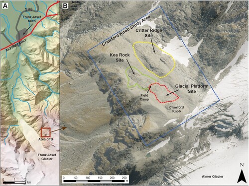
Figure 6. Orthophotograph, digital surface model (DSM) and digital 3-D outcrop model of the Glacial Platform site. A, orthophotograph with GSD of 4.3 mm over the outcrop site with inset panels B and C, enlarged views showing lithological layering in the schist, faults and quartz veins. D, digital surface model showing the elevation of the outcrop and hillshade model that highlights areas of smooth glacially eroded outcrop and gravel deposits at the site. E, Perspective view of 3-D model that uses the DSM with a draped orthophotograph to create a digital outcrop that can be used to map fault planes, schist layering, quartz veins and outcrop extent in GIS.
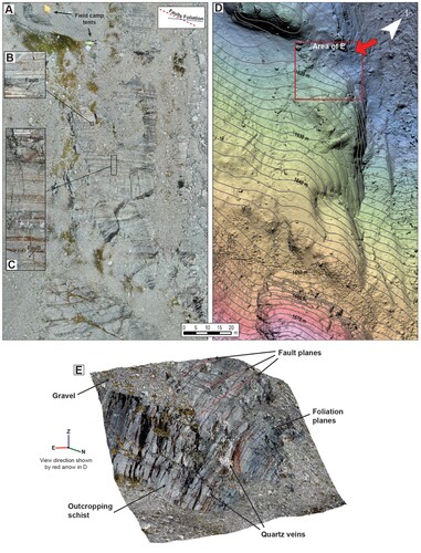
Figure 7. Orthophotograph images showing representative examples of each of the six lithological classes that we recognised in our mapping of the schist.
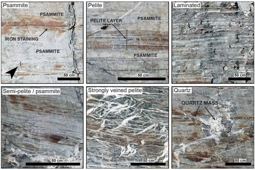
Figure 8. Geological map of the Glacial Platform outcrop site. Fault traces are colour-coded according to the mapping process used to locate them (mapped in situ with RTK GPS, shown in black; or virtually in GIS, shown in red). Rock type in the schist is assigned to six lithological classes (see legend and the main text). Black arrows depict the local dip direction of the generally sub-vertical faults. Inset Maps: A, enlarged part of the map showing a fault offsetting lithological layers in the schist. B, enlarged view of high-resolution orthophotographic image derived from RPAS data. The image shows faults offsetting lithological layers (dark and light bands) in the schist. C, RGB analysis used to identify white-coloured pixels in quartz veins (here rendered in pink), psammitic schist (yellow-green), and pelite (blue). D, enlarged part of the map showing representative detail at the metre scale, including coding of fault termination types (see adjoining legend), and local dip-directions and dip angles of faults (arrow symbols). Locations of Transect A and Transect B are shown with heavy black lines, with the several inferred fault-spacing domains approximately located by text labels. The topography of the outcrop outside of the geologically mapped area is depicted in greyscale as a hillshade DSM.
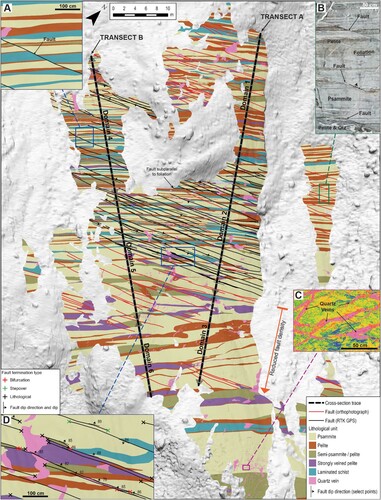
Figure 9. Lower hemisphere equal-area stereographic projections of structural orientations measured in the field at Crawford Knob. Parts A, B, and C plot poles to planar data (black dots), contours of the poles, and a great circle to depict the mean attitude of the planes (identified with label as a strike/dip/dip direction). A, predominant Alpine Schist foliation. B, deformed quartz-rich veins embedded in the Alpine Schist. C, brittle-ductile faults cross-cutting the Alpine Schist foliation and the veins. D, plots and contours calcite-quartz fibre lineations coating fault planes (black dots) and specifies the mean direction of these (red dot with labelled trend/plunge). E, plots the mean attitude of each of the above structures as a great circle or lineation together with the contoured poles of the measured faults (same as in C). Data plots and calculations were made using Stereonet 10 (Allmendinger Citation2020); contour intervals of 5 calculated using 1% of area; mean plane and line values from Bingham analysis; conical best fit half apical angle (CBFHA).
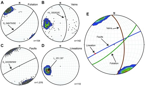
Figure 10. Outcrop photograph from RPAS illustrating offset quartz veins and lithological boundaries across faults. Example offset features paired by colour for each fault and of faults terminating at lithological boundaries and fault stepovers. Offsets are measured in the GIS (in the horizontal plane).
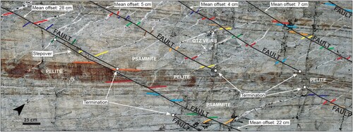
Figure 11. Histogram of average apparent offset in the horizontal plane of mapped faults at the Glacial Platform site. These offsets of quartz veins and foliation planes/lithological layers were measured using orthophotographs in the GIS. The counts represent the average horizontal offset obtained from multiple offset data for each fault (n = 265 individual faults, based on a total of 1032 offset marker observations). The median offset is 0.104 m and 50% of offsets lie between 0.066 and 0.21 m.
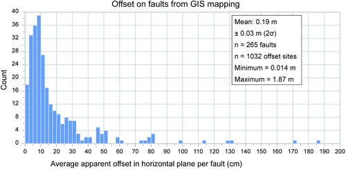
Figure 12. Simplified geological cross-sections for Transect A (above) and Transect B (below) viewed from the northeast (for location see ). No vertical exaggeration. The boundaries of the labelled fault domains are defined by spatial changes in mean fault spacing as revealed on a cumulative fault frequency plot (see Appendix 2). Domains 1 and 4; 2 and 5; and 3 and 6 (respectively) are approximate along-strike equivalents to each other between the two transects (see ).
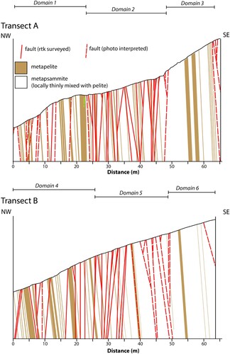
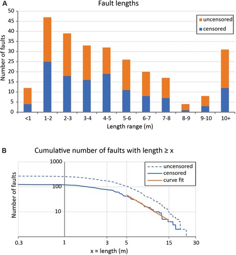
Figure 13. A, Histogram of apparent fault trace lengths where the number of faults between 0-1 m, 1-2 m, etc, are binned and plotted. Orange colour represents minimum (uncensored) fault length for faults that intersected the edge of the outcrop (i.e. the fault trace disappeared under gravel, such that the total fault length was greater than measured), whereas blue colour indicates lengths only for censored faults that were fully contained within the outcrop (i.e. we could measure the entire length with fault termination points at either end). The minimum and maximum censored fault lengths are (0.36, 20 m); whereas if we include uncensored faults these values are (0.5, 32 m). B, Cumulative frequency plot with the y-axis plotting the number of censored (thick blue line) and uncensored (thin dashed line) faults having a length greater than or equal to the length that is specified along the x-axis. These curves suggest a log-normal fault length distribution, although the flattened curve shape at small lengths (< 0.5 m) probably at least in part reflects undersampling as discussed in the text. The orange line shows the censored fault log-log fit between 5 and 15 m where faults are not under-sampled, with an equation (for cumulative number of faults y with length ≥ x) of y = 1478 x−2.134 (R-squared = 0.98). This corresponds to a power-law fit with an exponent of ∼ 3, as discussed in the text.
Data Availability Statement
The authors confirm that the data supporting the findings of this study are available within the article and its supplementary materials. The appendices are available for download at https://doi.org/10.6084/m9.figshare.22492936. Two supplementary data collections containing fault geometry and lithology (Supplementary Dataset 1) and the 3-D fault model (Supplementary Dataset 2) supporting the findings of this study are openly available at https://doi.org/10.21420/8VT4-2J73.
Acknowledgements
This study was funded by core funding to GNS Science and Victoria University of Wellington. The authors would like to thank the Department of Conservation for the help in permitting and providing radios; the Local Air Users Group at Franz Josef for their cooperation in providing permit conditions that allowed us to fly a remotely piloted aircraft in an area used by many helicopter companies; Neville Palmer and Garth Archibald for RTK GPS equipment preparation and training; and Te Runanga o Makaawhio (Komiti Taiao) for permission to access the field area. We acknowledge fruitful discussions with Simon Cox, David Prior, Virginia Toy, Steve Kidder, Andrew Cross, Cecile Massiot, Ruth Wightman, Susanne Grigull, and many others over the years. Mark Rattenbury, Cecile Massiot, Jack Williams and an anonymous reviewer provided constructive comments on the manuscript.