The potential for palaeoseismic and palaeoclimatic reconstructions from Lake Tennyson, North Canterbury, New Zealand

Figures & data

Figure 1. Tectonic and geologic setting of the Lake Tennyson area. A, Present day tectonic setting of New Zealand showing the main structural regimes. Extent of B is shown in shaded box. B, Major faults (labelled red lines) and historic earthquakes (circles) within the Marlborough Fault System. Location of C along the Awatere Fault is indicated by thick-bordered box (modified from (Rattenbury et al. 2006)). C, Geologic map for the area surrounding Lake Tennyson (modified from GNS Science, 2013). D) Oblique aerial imagery of Lake Tennyson indicating the inferred trace of the Awatere Fault (dashed red line) and the location of a fresh landslide head scarp through which it passes (indicated by orange arrow). The break in tree coverage immediately below the head scarp suggests recent failure. Image accessed from Google Earth®.

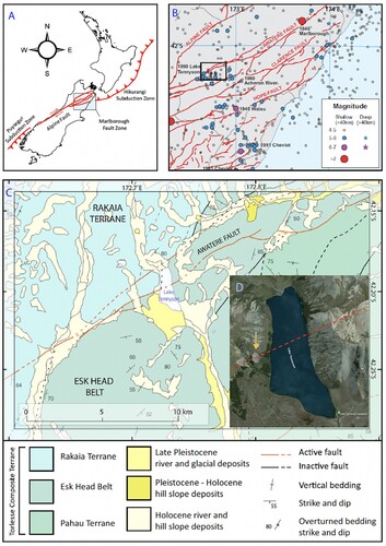
Figure 2. Bathymetric map of Lake Tennyson (5 m contour interval) overlaid on satellite imagery (accessed from Google Earth®). CHIRP profiles acquired for this study are indicated by orange lines, with bold blue lines showing traverse paths for CHIRP sub-bottom profiles discussed in text (e.g. C-C’ in Figure 3; G-G’ in Figure 4; B-B’ and O-O’ in Figure 5). Grey shaded area marks the bathymetric expression of the slump deposit discussed in text. Sediment core sample locations are indicated by red points. Locations of head scarp to the west of the lake and erosion gullies (black arrows on land) to the south are indicated on the satellite imagery. Bathymetric contours provided by Andrew Willsman (NIWA).

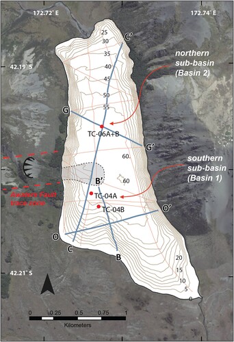
Figure 3. (top) Overview CHIRP imagery for the south to north trending profile showing the main structural features of Lake Tennyson described in text. Bathymetric map in Figure 2 shows path traversed to acquire this imagery as well as core sample locations. The hummocky deposit occurs where the 50 m contour protrudes into the centre of the lake and intersects the traverse line. Red box shows extent of imagery enhanced in the bottom panel. Dashed red lines indicate where cross sections seen in Figure 4, top (right red dashed line) and Figure 5, bottom (left red line) and intersect this profile. Thick black arrows indicate coring locations. (bottom) Enhanced CHIRP imagery for the hummocky deposit seen in the top panel (extent marked by red box). Internal structure of the deposit has a chaotic signal which extends to the basins to the north and south. Overlying the chaotic seismic facies in both basins are horizontal layers ranging between 0.75 and 1 m thickness. Red arrow indicates coring location.

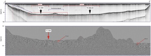
Figure 4. (top) CHIRP imagery which extends across Basin 2 of Lake Tennyson. Location of traverse line is shown on Figure 2. Red box shows extent of enhanced imagery presented in lower panel. Black arrow indicates coring location. Dashed red line indicates location where the CHIRP imagery from the top panel of Figure 3 crosses this traverse. (bottom) Enlarged and enhanced CHIRP imagery showing 1 m thick horizontally layered sediment overlying sediment with a chaotic structure (separated by dashed line) at a distal position relative to the hummocky deposit. Red arrow indicates coring location.

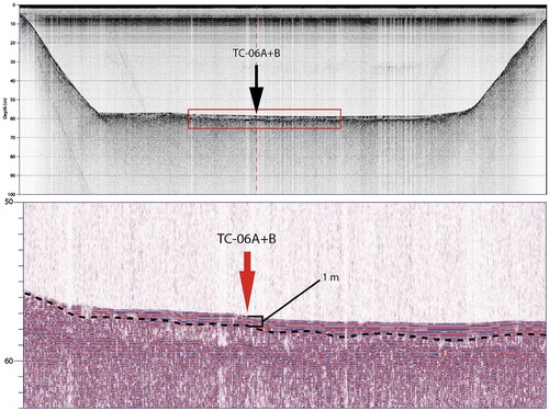
Figure 5. (top) CHIRP imagery across the thick sediment deposit on Lake Tennyson’s southern margin. Figure 2 shows the location of the traverse path. Black arrows point to a strong internal reflector within the overall structure indicating two phases of sediment emplacement. Red arrow points to upper boundary of the thick slope deposit where it extends beneath the upper horizontal sediments. Vertical dashed red lines mark locations at which Figures 3 and the lower left panel of this figure intersect this cross-section. (bottom left) CHIRP imagery showing the thick deposit of sediment on Lake Tennyson’s southern slope. Figure 2 shows traverse path for imagery. Black-bordered box indicates extent of enhanced imagery in the lower right panel. Dashed red line marks location at which the image in the top panel intersects this cross-section. Black arrow indicates location of core TC-04B. (bottom right) Enhanced CHIRP imagery from the bottom left panel (extent indicated by black-bordered box) showing the internally chaotic structure of the thick slope deposit. Above the dashed red line, an upper layer of bedded sediments (50 cm thick) parallel to the slope overlies the thick deposit. Note that the enlargement of CHIRP facies around TC-04B (lower right) displays evidence for multiple depositional events and sedimentation phases.

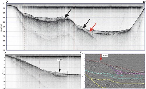
Figure 6. Summary logs and positions of radiocarbon samples for the Lake Tennyson sediment cores. Bathymetric map indicates coring sites. Radiocarbon dates are shown as conventional radiocarbon age (CRA) with the associated lab identifier, and their calibrated range can be found in Table 1 as cal. yr BP at 2σ from the SHCal20 curve (Hogg et al. 2020) as produced in Calib8.2. Ages marked * indicate samples measured using bulk carbon AMS. Arrow points to distinct interface between folded and horizontal layers in TC-06A. Dashed lines represent inferred correlation between cores based on the stratigraphic context of sediment layers (see text). Correlated sand layers in TC-06A and TC-06B are labelled S1 – S3.

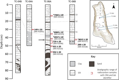
Figure 7. Analyses run on cores TC-04A (top), TC-04B and TC-06A(bottom). Summary stratigraphic log is shown with depth scale to the left, with grain size presented for TC-04A and B. Loss-on-ignition (LOI) was run for all cores, while Sulphur was only run for TC-04A and B. Total organic carbon (TOC), total nitrogen (TN), and carbon/nitrogen ratio (TOC/TN) for core TC-04A are also presented. Blue shaded area of TOC/TN indicates ratios between 4 and 10, indicative of aquatically-sourced sedimentary organic matter. Red marker to right of diagrams shows the stratigraphic range and position of radiocarbon samples. Radiocarbon dates are shown as conventional radiocarbon age (CRA) with the associated lab identifier, and their calibrated range can be found in Table 1 as cal. yr BP at 2σ from the SHCal20 curve (Hogg et al. 2020) as produced in Calib8.2.

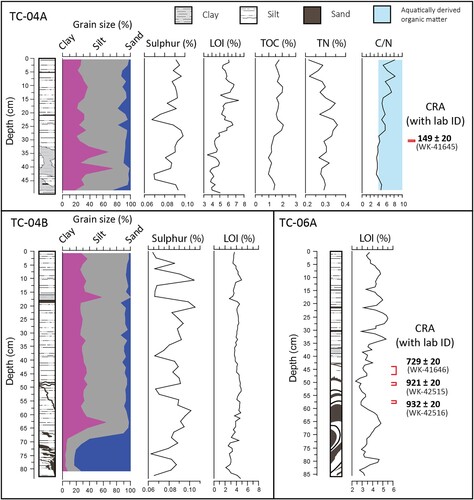
Figure 8. Micro-XRF core scanning data for core TC-06A. All elemental data is normalised to incoherent scattering (inc). Dashed line indicates depth below which sediments are deformed. Radiocarbon dates are shown as conventional radiocarbon age (CRA) with the associated lab identifier, and their calibrated range can be found in Table 1 as cal. yr BP at 2σ from the SHCal20 curve (Hogg et al. 2020) as produced in Calib8.2.

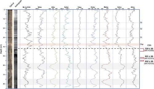
Figure 9. ITRAX-XRF data for core TC-06B. All individual elemental data is normalised to incoherent scattering. Radiocarbon dates are shown as conventional radiocarbon age (CRA) with the associated lab identifier, and their calibrated range can be found in Table 1 as cal. yr BP at 2σ from the SHCal20 curve (Hogg et al. 2020) as produced in Calib8.2.

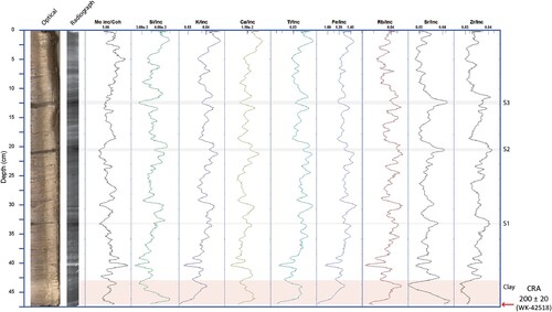
Figure 10. Ti-normalised elemental data and the Fe/Mn ratio for core TC-06A. Dashed line indicates depth below which, sediments are deformed. Radiocarbon dates are shown as conventional radiocarbon age (CRA) with the associated lab identifier, and their calibrated range can be found in Table 1 as cal. yr BP at 2σ from the SHCal20 curve (Hogg et al. 2020) as produced in Calib8.2.

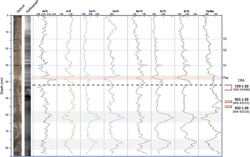
Figure 11. Ti-normalised elemental data and the Fe/Mn ratio for core TC-06B. Radiocarbon dates are shown as conventional radiocarbon age (CRA) with the associated lab identifier, and their calibrated range can be found in Table 1 as cal. yr BP at 2σ from the SHCal20 curve (Hogg et al. 2020) as produced in Calib8.2.

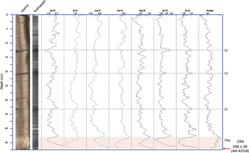
Table 1. Radiocarbon sample details and results for macroscopic organics and bulk sediment samples from the Lake Tennyson sediment cores. The asterisk indicates a calibrated age that overlaps with the modern part of the calibration curve (post 1950 CE). All calibrations undertaken with Calib8.2 and the SH20Cal curve.

Core ID	Depth (cm)	^14C sample identifier	CRA	Calibrated date range[s] (2σ)	Relative area under probability distribution	Median Probability age	Sample material	Context within core
TC-04A	30 −30.5	WK-41645	149 +/−20	1691–1728 cal AD	0.224	1853 cal AD	Bark	Thin, rigid, flat-lying piece of organic material protruding into centre of core.
				1808–1896 cal AD	0.543
				1902–1950 cal AD*	0.233
TC-06A	44.5–47.5	WK-41646	729 +/−20	1280–1318 cal AD	0.556	1311 cal AD	Wood	Piece of wood sitting vertically in centre of core. Occurs within folded layers 6cm below distinct non-deformed clay layer.
				1356–1384 cal AD	0.444
TC-06A	54–55	WK-42515	921 +/−20	1052–1061 cal AD	0.028	1177 cal AD	Leaf fragments	Within deformed sediment.
				1069–1081 cal AD	0.049
				1149–1219 cal AD	0.922
TC-06A	57–58	WK-42516	932 +/−20	1049–1084 cal AD	0.202	1167 cal AD	Leaf fragments	Within deformed sediment.
				1144–1217 cal AD	0.798
TC-06B	Base	WK-42518	200 +/−20	1667–1701 cal AD	0.265	1754 cal AD	Leaf	Immediately below clay layer at base of core.
				1721–1787 cal AD	0.481
				1791–1811 cal AD	0.152
				1836–1849 cal AD	0.027
				1867–1878 cal AD	0.023
				1926–1950 cal AD*	0.052
TC-06A	13–14	WK-42512	7365 +/−20	6230–6213 cal BC	0.181	6157 cal BC	Bulk sediment	Immediately above top sand layer.
				6191–6166 cal BC	0.220
				6148–6091 cal BC	0.599
TC-06A	35–36	WK-42513	6969 +/−22	5889–5731 cal BC	1.000	5806 cal BC	Sieved sediment	Immediately above clay layer.
TC-06A	41–42	WK-42514	4557 +/−20	3361–3262 cal BC	0.337	3210 cal BC	Bulk sediment	Above deformation (where arrow is pointing in Figure 6).
				3249–3100 cal BC	0.663
TC-06B	42–43	WK-42517	8015 +/−20	7046–6768 cal BC	0.963	6912 cal BC	Bulk sediment	Immediately above clay layer.
				6757–6751 cal BC	0.007
				6721–6702 cal BC	0.030

Table 2. Cross correlation results of selected µ-XRF derived elements from Lake Tennyson cores. Strong correlations are noted for TC-06a series meeting or exceeding a p-value threshold of 0.05 (95% confidence interval).

	K	Ca	Ti	Mn	Fe	Rb	Sr	Zr
TC-06a
Si	0.62	0.64	0.54	0.38	0.48	0.10	−0.11	−0.13
K		0.71^a	0.90^a	0.75^a	0.88^a	0.30	−0.31	−0.11
Ca			0.63	0.49	0.56	0.11	−0.08	−0.14
Ti				0.74^a	0.90^a	0.38	−0.32	−0.12
Mn					0.84^a	0.07	−0.54	−0.22
Fe						0.32	−0.50	−0.23
Rb							0.09	0.08
Sr								0.56
TC-06b
Si	0.51	0.6	0.48	0.33	0.36	0.13	0.01	0.03
K		0.62	0.83	0.73	0.87	0.4	−0.31	0.05
Ca			0.53	0.41	0.5	0.18	−0.04	−0.09
Ti				0.69	0.84	0.38	−0.28	0.07
Mn					0.81	0.19	−0.33	0.06
Fe						0.37	−0.46	0
Rb							−0.1	0.06
Sr								0.35

^a Strong correlations (r ≥ 0.7 or r ≤ −0.7).

Rattenbury MS, Townsend DB, Johnston MR. 2006. Geology of the Kaikoura area. Lower Hutt, Wellington: Institute of Geological & Nuclear Sciences 1:250 000 geological map 13. GNS Science, 70.

 Google Scholar

Hogg AG, Heaton TJ, Hua Q, Palmer JG, Turney CS, Southon J, Bayliss A, Blackwell PG, Boswijk G, Bronk Ramsey C, et al. 2020. SHCal20 Southern Hemisphere Calibration, 0–55,000 Years cal BP. Radiocarbon. 62(4):759–778. doi:10.1017/RDC.2020.59.

 Web of Science ®Google Scholar

Data availability statement

All ITRAX and bathymetric data will be made available on reasonable request.