Bayesian Design of Experiments Using Approximate Coordinate Exchange

Figures & data

Figure 1. Poisson example in Section 2.4. (a), (c) expected utility U(x) against x, with Monte Carlo evaluations $\tilde{U}\left(x\right)$ at the coordinate-design points and GP emulator $\widehat{U}\left(x\right)$; (b), (d) median probability p†_I of accepting the candidate point against the current point, x^C. [Coordinate-designs are: ξ¹ for (a), (b); ξ² for (c), (d)].

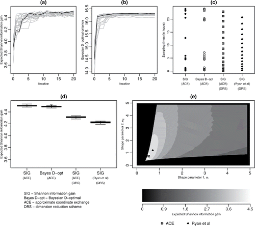
Figure 2. (a), (b) Trace plots of $\tilde{U}\left({\mathit{}\mathbf{\delta }}^C\right)$ for each iteration of the ACE algorithm for SIG and pseudo-Bayesian D-optimality utilities, respectively; in each plot, the black line shows the trace of the expected utility for the best design; (c) designs found from the ACE algorithm: unrestricted SIG-optimal, pseudo-Bayesian D-optimal, Beta DRS SIG-optimal, together with the Ryan et al. (2014) Beta DRS SIG-optimal designs; (d) boxplots for 20 evaluations of ${\tilde{U}}^S\left({\mathit{}\mathbf{\delta }}^{★}\right)$ for designs from these four methodologies; (e) approximate expected utility surface for SIG as a function of the Beta DRS parameters; parameter values corresponding to the Ryan et al. (2014) and the ACE DRS designs are marked.

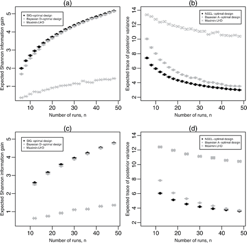
Figure 3. Results from 20 evaluations of (a) ${\tilde{U}}^S\left(\mathit{}\mathbf{\delta }\right)$ for SIG-optimal, pseudo-Bayesian D-optimal, and maximin Latin hypercube designs, and (b) $-{\tilde{U}}^V\left(\mathit{}\mathbf{\delta }\right)$ for NSEL-optimal, pseudo-Bayesian A-optimal, and maxmin Latin hypercube designs, for homogenous logistic regression; (c) and (d) show the same evaluations for hierarchical logistic regression. For the latter two plots, for each value of n, 20 different random assignments are made of the points of the Latin hypercube design to the G groups, and each resulting design is evaluated 20 times. For each design, the central plotting symbol denotes the mean expected Shannon information gain or expected average posterior variance, with the two horizontal lines denoting the minimum and maximum of these quantities.

Table 1. Approximate posterior model probabilities, π(u | y), for the beetle mortality data.

u	Link function	Linear predictor	π(u | y)
1	Logit	1st order	0.0216
2	Logit	2nd order	0.0686
3	C-log-log	1st order	0.7580
4	C-log-log	2nd order	0.0612
5	Probit	1st order	0.0304
6	Probit	2nd order	0.0602

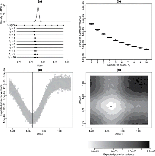
Figure 4. (a) Posterior density for LD50, the original experimental doses and optimal doses (in mg/L) for each value of n₀; (b) boxplots of 20 evaluations of $-{\tilde{U}}^V\left({\mathit{}\mathbf{\delta }}^{★}\right)$ for each n₀ for the NSEL-optimal designs; (c) negative approximate expected utility $-{\tilde{U}}^V\left(\mathit{}\mathbf{\delta }\right)$ against dose for n₀ = 1; the vertical line indicates δ^⋆. (d) negative approximate expected utility $-{\tilde{U}}^V\left(\mathit{}\mathbf{\delta }\right)$ against dose for n₀ = 2; ⊠ indicates δ^⋆.

Ryan, E. G., Drovandi, C. C., Thompson, M. H., and Pettitt, A. N. (2014), “Towards Bayesian Experimental Design for Nonlinear Models That Require a Large Number of Sampling Times,” Computational Statistics and Data Analysis, 70, 45–60.

 Web of Science ®Google Scholar