Optimisation-based coordination of connected, automated vehicles at intersections

Figures & data

Figure 1. Illustrations of collision avoidance conditions. (a) Illustration of Assumption 2.2 and the Conflict Zones (red boxes); (b) scheme of the SICA condition (3(3) $(x_i(t),x_j(t))\notin {\hat{\mathcal{B}}}_{r,ij}=\{(x_i,x_j)|p_i\in [p_{r,i}^{\mathrm{in}},p_{r,i}^{\mathrm{out}}],p_j\in [p_{r,j}^{\mathrm{in}},p_{r,j}^{\mathrm{out}}]\},$(3) ): ${\hat{\mathcal{G}}}_i(p_i(t))$ shown as boxes around the vehicles and (c) conservativeness induced by rectangular outer approximations.

Figure 2. Scenario for the performance evaluation.

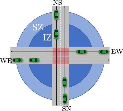
Table 1. General parameters.

Type	Symbol	Value	Unit
SZ Start	$p_{\mathrm{SZ}}^{\mathrm{e}}$	−350	m
SZ Stop	$p_{\mathrm{SZ}}^{\mathrm{d}}$	250	m
IZ Start	$p_{\mathrm{IZ}}^{\mathrm{e}}$	−200	m
IZ Stop	$p_{\mathrm{IZ}}^{\mathrm{d}}$	250	m
Car Gen. Prob.	$p^{\mathrm{Car}}$	0.9
Truck Gen. Prob.	$p^{\mathrm{Truck}}$	0.1
Initial/Set Speed	$v^{\mathrm{e}}$	70	km/h
Discretisation size	$\mathrm{\Delta }t$	0.2	s
Prediction Horizon	K	100
RECA Safety distance	ε	1.5	m
T.L. Cycle time	C	20	s
Air density	ρ	1.225	${\mathrm{kg}/\mathrm{m}}^3$
Acc. due to gravity	g	9.81	${\mathrm{m}/\mathrm{s}}^2$

Table 2. Vehicle parameters.

		Value
Type	Symbol	Car	Truck	Unit
Mass	$m_i$	1.7	20	${10}^3$ kg
Length	$L_i$	4.8	16.5	m
Width	$W_i$	1.77	2.55	m
Speed Dev. Weight	$Q_i$	1
Control Use Weight	$R_i$	1
Acceleration L.B.	$a_i^{min}$	$-3$		${\mathrm{m}/\mathrm{s}}^2$
Acceleration U.B.	$a_i^{max}$	3		${\mathrm{m}/\mathrm{s}}^2$
Gear ratio	$G_i$	7.94	15
Wheel radius	$r_i^{\mathrm{w}}$	0.35		m
Projected Front Area	$a_i$	2.3	4	${\mathrm{m}}^2$
Air drag coef.	$c_i^{\mathrm{d}}$	0.32	0.7
Rolling resistance coef.	$c_i^{\mathrm{rr}}$	0.015
Max Power	$P_i^{max}$	80	400	kW
Max Torque	$M_i^{max}$	250	2000	kNm
Max Motor Speed	${\omega }_i^{max}$	10	15	kRPM

Figure 3. Components of the quadratic objective. T.L. denotes the traffic light controller.

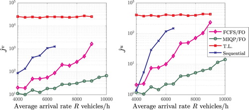
Figure 4. Energy cost of coordination: percentage increase ${\hat{E}}^{\mathrm{\%}}$ (solid line, right axis); and CoC increase ${\hat{E}}^{\mathrm{CoC}}$ (pale lines, left axis). Colour coding as in Figure 3.

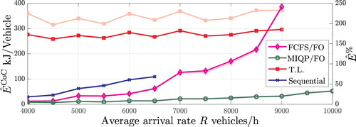
Figure 5. Travel time delay compared to the Overpass solution.

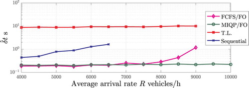
Figure 6. Estimate of the distribution of the observed $\delta t_i$ for R = 6000 vehicles/h.

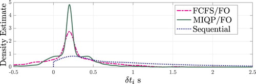
Figure 7. Average velocity (coloured lines) and velocity intervals (grey surface) in a scenario with R = 6000 vehicles/hour.

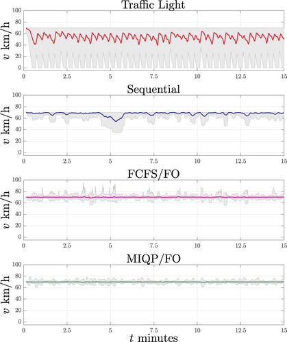
Figure 8. Position-velocity trajectories of one vehicle from the scenario with R = 6000 vehicles/hour. The grey bar corresponds to positions inside the intersection, 0 being the centre, whereas the grey line demarcates the beginning of the IZ.

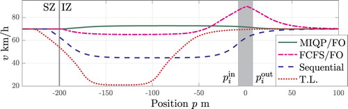
Figure 9. Speed profiles of Trucks (dark) and Cars (pale). The solid bars and the two vertical lines mark the intersection for Cars (dark) and Trucks (light) and the start of the SZ and IZ, respectively.

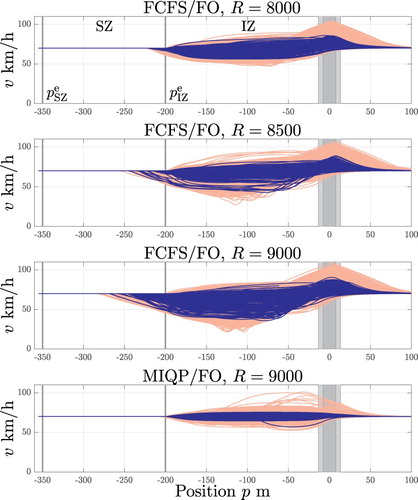
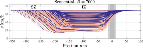
Figure 10. Velocity profiles for vehicles in the scenario with R = 7000, where the sequential controller failed. Colouring as in Figure 9.