Improved curving performance of an innovative two-axle vehicle: a reasonable feedforward active steering approach

Figures & data

Table 1. Unit properties.

Property	Metro Madrid class 8000	Innovative 2-axle vehicle
Maximum speed	120 km/h	120 km/h
Number of vehicles	3	5
Train length	55 m	60 m
Payload per metre	1000 kg/m	1000 kg/m
Tare weight per metre	1900 kg/m	1500 kg/m

Figure 1. Suspension position (Left), anti-roll bar implementation in SIMPACK (Right).

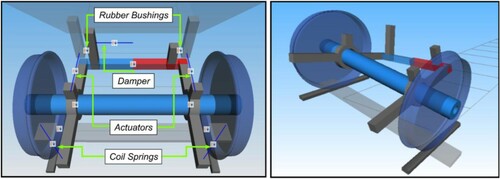
Figure 2. Top view of the innovative vehicle (Scheme).

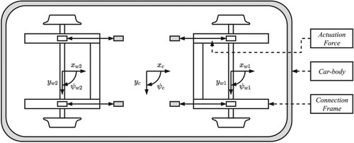
Figure 3. Speed distribution [km/h] as function of curve radius and NLA.

Figure 4. Equivalent conicity as function of wheel lateral displacement.

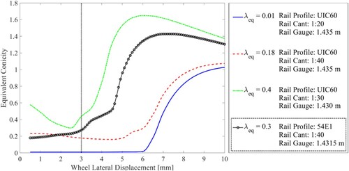
Figure 5. Reference tracking errors: Lateral Displacement (Left), attack angle (right). The vertical scale is made sectional logarithmic to highlight the tails (0–5% and 95–100%) of the distribution.

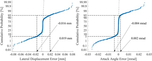
Figure 6. Performance comparison between the feedback approaches in terms of normalised cumulative dissipated energy. The CDE values are expressed as percentage of the maximum achieved one per wheelset. Each bar groups the results for each feedback approach.

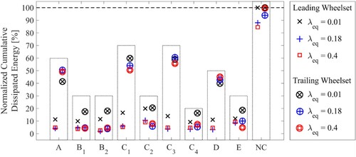
Figure 7. Leading wheelset lateral displacement with a controller designed for ${\lambda }_{eq}=0.18$ shown for different equivalent conicities against normalised time: speed equal to 10 km/h (Left) and speed equal to 82 km/h (Right).

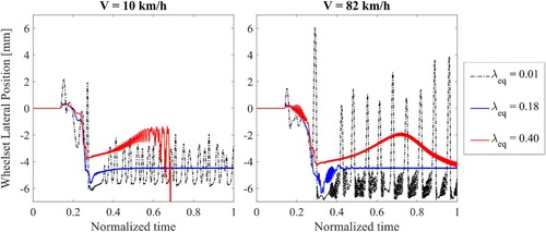
Figure 8. Decision table for selecting the feedback approach giving the lowest cost for equivalent conicity 0.01 (Left), 0.18 (Centre) and 0.40 (Right).

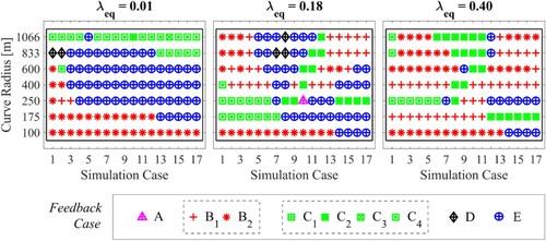
Figure 9. Feedforward control scheme.

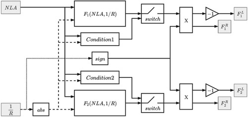
Table 2. Approximation functions coefficients. Each column gives the possible combinations of the exponents of Equation (10). Each row gives the coefficients that must be multiplied by the variables (NLA and 1/R) as shown in Equation (11).

	Leading wheelset				Trailing wheelset
	n=1, m=1	n=2, m=1	n=1, m=2	n=2, m=2	n=1, m=1	n=2, m=1	n=1, m=2	n=2, m=2
$k_1$	∖	∖	∖	8.99e8	∖	∖	∖	1.10e9
$k_2$	∖	∖	9.62e8	9.87e8	∖	∖	5.74e8	6.82e8
$k_3$	∖	∖	8.82e7	−5.28e7	∖	∖	6.16e8	4.21e8
$k_4$	∖	8.22e5	∖	−9.97e6	∖	−5.30e6	∖	−1.56e7
$k_5$	2.22e6	2.03e6	−7.79e6	−8.11e6	−2.75e6	−1.55e6	−9.00e6	−9.42e6
$k_6$	1.43e7	1.42e7	1.33e7	1.49e7	1.51e7	1.56e7	8.51e6	1.10e7
$k_7$	∖	−2.17e3	∖	1.47e4	∖	1.17e4	∖	3.05e4
$k_8$	−1.85e4	−1.78e4	−1.39e3	−1.83e3	−4.49e3	−8.78e3	5.33e3	3.41e3
$k_9$	3.60e3	3.76e3	4.98e3	2.88e3	−1.14e4	−1.21e4	−1.03e3	−5.19e3

Figure 10. Performance comparison between the feedforward approaches in terms of normalised cumulative dissipated energy. Each bar groups the results for each feedforward approximation function.

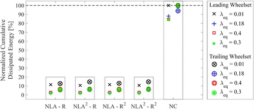
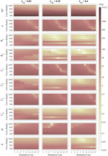
Figure 11. Tγ distribution for the not controlled vehicle (NC) and the feedforward controlled (FF). Leading wheelset (Top) and trailing wheelset (Bottom).

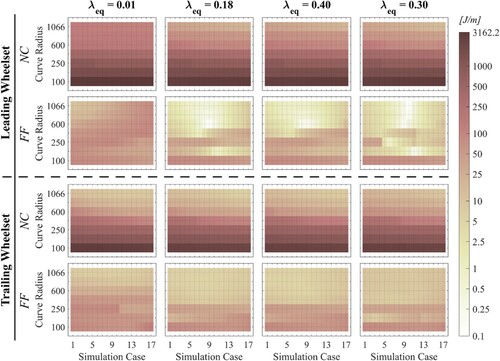
Figure 12. Time simulation results on two different running cases comparing the controlled and not controlled vehicle: equivalent conicity 0.18, curve radius 175 m, speed 54 km/h (Top), equivalent conicity 0.3, curve radius 711 m, speed 94 km/h (Bottom), leading wheelset (Left) and trailing wheelset (Right).

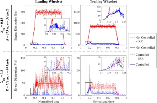
Figure A1. Tγ distribution for feedback approaches: leading wheelset.

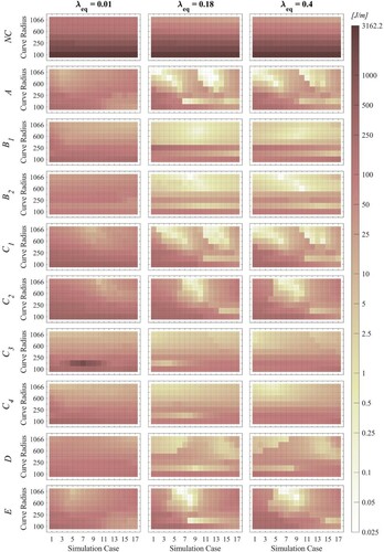
Figure A2. Tγ distribution for feedback approaches: trailing wheelset.