Modeling of In-Line Tube Banks Inside Advanced Gas-Cooled Reactor Boilers

Figures & data

Table 1. All configurations of cases run in this study, delineated by turbulence models used, wall treatment strategies, and the corresponding grids utilized as listed under Figure 3.

Turbulence model	Wall treatment(s)	Grid (Corresponding Figure, cell count)
k-ε LP	Standard wall function and analytical wall function	High-Re Grid (Figure 3a, cell count: 528,000)
k-ω SST	Resolved boundary layer to y* ≤ 1	Low-Re Grid (Figure 3b, cell count: 1,456,000)
ϕ-f	Resolved boundary layer to y* ≤ 1	Low-Re Grid (Figure 3b cell count: 1,456,000)
Rij-ε SSG	Standard wall function and analytical wall function	High-Re Grid (Figure 3a, cell count: 528,000)
Rij-ε EB-RSM	Resolved boundary layer to y* ≤ 1	Low-Re Grid (Figure 3b, cell count: 1,456,000)
LES (Dynamic)	Resolved boundary layer to Δy* ≤ 1 (including Δx^+ < 20 and Δz^+< 40 globally)	LES Grid (Figure 3c, cell count: ∼5,200,000)

Figure 1. Square and triangular primitive units for banks of tubes, corresponding to in-line (left) and staggered (right) banks.

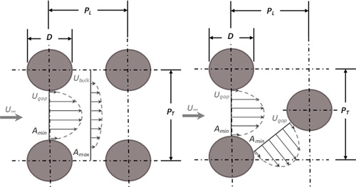
Figure 2. Sketch adapted from [6] with permission, showing three of the five flow patterns typically exhibited by in-line tube banks with variable longitudinal ($\frac{P_T}{D}$) and transverse pitches ($\frac{P_L}{D}$), where the shaded section indicates an impossible arrangement.

Figure 3. Meshes used for the periodic tube domain, representing an indefinite square in-line tube bank with pitch-to-diameter ratio equal to 1.6.

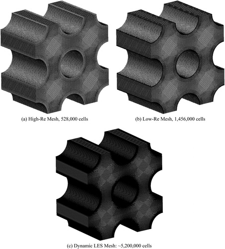
Figure 4. Plots showing mesh insensitivity using the k-ω SST model at resolutions of 4, 8, 16, and 20 spanwise cells per tube diameter in length, with corresponding cell counts of 291,200, 582,400, 1,164,800, and 1,456,000, compared to Aiba et al. [17] and West [4].

Figure 5. Plot demonstrating the convergence of the simulation toward the desired Reynolds number in time, where time-averaging begins once the variable Reynolds number reaches to within ±10 of the target.

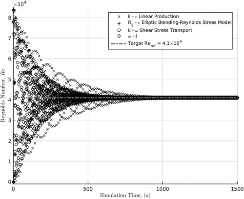
Figure 6. Plot showing the periodicity of the fluctuating lift and drag coefficient signals behind the central tube of the flow domain using the R_ij-ε SSG model, indicating that periodic conditions are reached that are appropriate for time and spatial averaging.

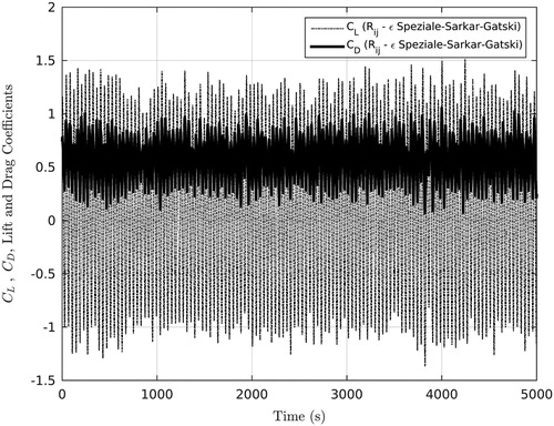
Figure 7. Plot showing the Fast Fourier Transform of the lift signal under Fig. 6, indicating that the dominant Strouhal number is ∼0.162 (St = fD/U_bulk), equivalent to a frequency of 2.458 Hz, where time-averaging takes place for all following results over 3,500 s of simulation time.

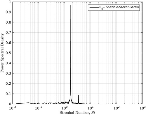
Figure 8. Plot showing the time-averaged static pressure coefficient distribution about the central tube in the three-dimensional 2 × 2 periodic array, as obtained by the low-Reynolds number turbulence models tested, compared with the experimental data of Aiba et al. [17].

Figure 9. Plot showing the time-averaged static pressure coefficient distribution about the central tube in the three-dimensional 2 × 2 periodic array, as obtained by the k-ε LP turbulence model using the standard wall function and the AWF [18], and Dynamic LES, compared with the data of Aiba et al. [17].

Figure 10. Plot showing the time-averaged static pressure coefficient distribution about the central tube in the three-dimensional 2 × 2 periodic array, as obtained by the R_ij-ε SSG turbulence model using the standard wall function and the AWF [18], and Dynamic LES, compared with the data of Aiba et al. [17].

Figure 11. Plot showing the time-averaged Nusselt number distribution about the central tube in the three-dimensional 2 × 2 periodic array, as obtained by the low-Reynolds number turbulence models tested, compared with the heat transfer data of Aiba et al. [17].

Figure 12. Plot showing the time-averaged Nusselt number distribution about the central tube in the three-dimensional 2 × 2 periodic array, as obtained by the k-ε LP turbulence model using the standard wall function and the AWF [18], and Dynamic LES, compared with the heat transfer data of Aiba et al. [17].

Figure 13. Plot showing the time-averaged Nusselt number distribution about the central tube in the three-dimensional 2 × 2 periodic array, as obtained by the R_ij-ε SSG turbulence model using the standard wall function and the AWF [18], and Dynamic LES, compared with the heat transfer data of Aiba et al. [17].

Figure 14. Plot showing the time-averaged friction coefficient distribution about the central tube in the three-dimensional 2 × 2 periodic array, as obtained by the low-Reynolds turbulence models tested against the prediction made via Dynamic LES.

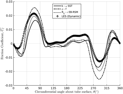
Figure 15. Plot showing the time-averaged friction coefficient distribution about the central tube in the three-dimensional 2 × 2 periodic array, as obtained by the k-ε LP turbulence model using the standard wall function and the AWF [18] against the prediction made via Dynamic LES.

Figure 16. Plot showing the time-averaged friction coefficient distribution about the central tube in the three-dimensional 2 × 2 periodic array, as obtained by the R_ij-ε LP turbulence model using the standard wall function and the AWF [18] against the prediction made via Dynamic LES.

Figure 17. Diagrams representing the momentum (left) and thermal (right) domains considered by the smooth-walled Analytical Wall Function on a cell-by-cell basis in the near-wall region of flow.

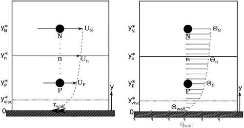
Figure 18. Plot showing the close agreement between the Analytical Wall Function and DNS data for a statistically-steady, two-dimensional turbulent momentum boundary layer in a channel flow at Re_τ = 395 [29] and Re_τ = 950 [30].

Figure 19. Plot showing the close agreement between the Analytical Wall Function and DNS data for a statistically-steady, two-dimensional turbulent thermal boundary layer in a channel flow at Re_τ = 395 at various Prandtl numbers [29].

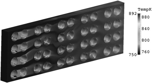
Figure 20. Filled thermal contours showing a snapshot of the unsteady left-to-right flow in a non-periodic 40-tube platen subject to confining walls, calculated using N8 HPC resources on a block-structured mesh numbering ∼9.8 M cells using the k-ε LP turbulence model in Code_Saturne.

S. Ishigai and E. Nishikawa, “Structure of gas flow and its pressure loss in tube banks with tube axes normal to flow,” Trans. JSME, vol. 43, no. 373, pp. 3310–3319, 1977. DOI: 10.1299/kikai1938.43.3310.

 Google Scholar

S. Aiba, H. Tsuchida, and T. Ota, “Heat transfer around tubes in inline tube banks,” Bull. JSME, vol. 25, no. 204, pp. 919–924, Jun. 1982. DOI: 10.1299/jsme1958.25.919.

 Google Scholar

A. West, “Assessment of computational strategies for modelling in-line tube banks”, Ph.D. thesis, The University of Manchester, 2013

 Google Scholar

K. Suga, T. J. Craft, and H. Iacovides, “An analytical wall-function for turbulent flows and heat transfer over rough walls,” Int. J. Heat Fluid Flow, vol. 27, no. 5, pp. 852–866, 2006. DOI: 10.1016/j.ijheatfluidflow.2006.03.011.

 Web of Science ®Google Scholar

H. Kawamura, H. Abe, and Y. Matsuo, “DNS of turbulent heat transfer in channel flow with respect to Reynolds and Prandtl number effects,” Int. J. Heat Fluid Flow, vol. 20, no. 3, pp. 196–207, 1999. DOI: 10.1016/S0142-727X(99)00014-4.

 Web of Science ®Google Scholar

S. Hoyas and J. Jiménez, “Reynolds number effects on the Reynolds-stress budgets in turbulent channels,” Phys. Fluids, vol. 20, no. 10, pp. 101511, 2008. DOI: 10.1063/1.3005862.

 Web of Science ®Google Scholar