2,064
Views
38
CrossRef citations to date
0
Altmetric
Special Issue: Hydrological Science for Environmental Flows

Quantifying flow–ecology relationships with functional linear models

Quantification des relations débit–écologie par des modèles linéaires fonctionnels

, &
Pages 629-644 | Received 25 Oct 2012, Accepted 16 Aug 2013, Published online: 10 Apr 2014

Figures & data

Fig. 1 Comparison of observed discharge and four key summary statistics over a 12-month period for two different systems in the USA. The two very different hydrographs have very similar hydrologic metrics over the interval shown.
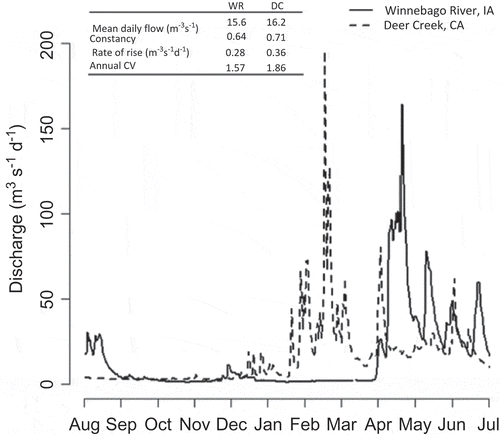
Fig. 1 Comparison of observed discharge and four key summary statistics over a 12-month period for two different systems in the USA. The two very different hydrographs have very similar hydrologic metrics over the interval shown.

Fig. 2 Map of the USA showing the location of sampling sites for the two case studies. Case study #1 comprises a database of fish species occurrences from one-time standardized surveys at 32 free-flowing streams across the midwestern USA. Case study #2 consists of a single sample of the density of three different species collected each year over 18 years from secondary channels in a single 138-km-long reach of the San Juan River in New Mexico and Utah from 1993 to 2010.
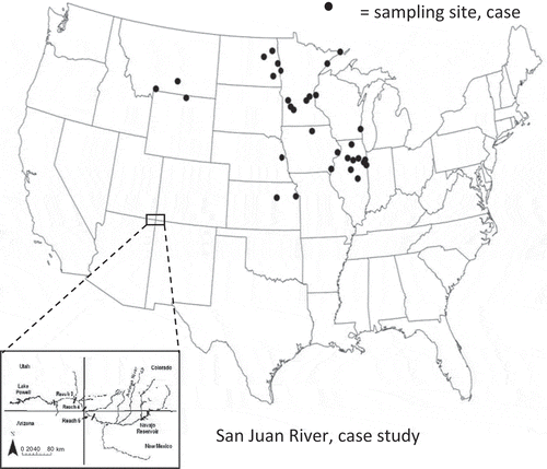
Fig. 2 Map of the USA showing the location of sampling sites for the two case studies. Case study #1 comprises a database of fish species occurrences from one-time standardized surveys at 32 free-flowing streams across the midwestern USA. Case study #2 consists of a single sample of the density of three different species collected each year over 18 years from secondary channels in a single 138-km-long reach of the San Juan River in New Mexico and Utah from 1993 to 2010.

Fig. 3 Observed discharge in the San Juan River (log scale) for two different years (thick dashed line) with the functional predictor variable used for each year overlaid (thin dotted line).
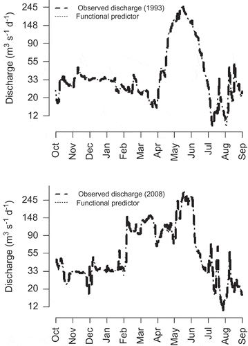
Fig. 3 Observed discharge in the San Juan River (log scale) for two different years (thick dashed line) with the functional predictor variable used for each year overlaid (thin dotted line).

Fig. 4 Five hypothetical environmental flow scenarios using the approximately 370 000 ML of water available for such use in the Navajo Dam. In each scenario the entire volume of water is delivered as part of a single-flow release over 30, 60 or 90 days, which equates to releases at mean daily flow rates of 143, 71 and 48 m-3 s-1, respectively.
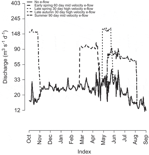
Fig. 4 Five hypothetical environmental flow scenarios using the approximately 370 000 ML of water available for such use in the Navajo Dam. In each scenario the entire volume of water is delivered as part of a single-flow release over 30, 60 or 90 days, which equates to releases at mean daily flow rates of 143, 71 and 48 m-3 s-1, respectively.

Fig. 5 Functional regression coefficients for the proportion of the three life-history strategies—periodic, opportunistic and equilibrium—in streams across the midwestern USA. The functional coefficients quantify the relationship between the richness of each life-history strategy and river flow on each day of the year prior to sampling. Streams with higher runoff at times of the year when the coefficient is above zero tend to have higher proportions of each strategy during the summer sampling period. In contrast, streams with higher runoff when the coefficient is below zero tend to have lower proportions of each strategy during the summer sampling period. The solid line represents the parameter estimate, with dotted lines being the 95% confidence interval. The p values on each plot indicate the significance of that model based on the permutation tests described in the “Methods” section.
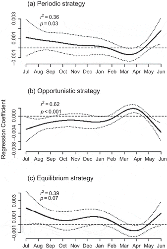
Fig. 5 Functional regression coefficients for the proportion of the three life-history strategies—periodic, opportunistic and equilibrium—in streams across the midwestern USA. The functional coefficients quantify the relationship between the richness of each life-history strategy and river flow on each day of the year prior to sampling. Streams with higher runoff at times of the year when the coefficient is above zero tend to have higher proportions of each strategy during the summer sampling period. In contrast, streams with higher runoff when the coefficient is below zero tend to have lower proportions of each strategy during the summer sampling period. The solid line represents the parameter estimate, with dotted lines being the 95% confidence interval. The p values on each plot indicate the significance of that model based on the permutation tests described in the “Methods” section.

Fig. 6 Functional regression coefficients for the density of speckled dace, flannelmouth sucker and red shiner in the San Juan River. See Fig. 5 caption for an explanation of the functional coefficient.
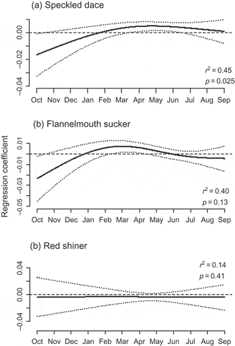
Fig. 6 Functional regression coefficients for the density of speckled dace, flannelmouth sucker and red shiner in the San Juan River. See Fig. 5 caption for an explanation of the functional coefficient.

Fig. 7 (a) Functional and (b) scalar regression coefficients for the second model fitted for red shiner. This model provided a much better fit to the data than the first model for red shiner (Fig. 5(c)). As with the functional coefficient, the scalar regression coefficients are shown with their approximate 95% confidence intervals, neither of which cross zero, indicating a significant relationship. The two scalar predictors are number of days in summer <14 m-3 s-1 (LFS) and the number of days over the 75th percentile of flow in autumn (HFA).
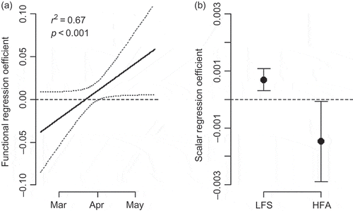
Fig. 7 (a) Functional and (b) scalar regression coefficients for the second model fitted for red shiner. This model provided a much better fit to the data than the first model for red shiner (Fig. 5(c)). As with the functional coefficient, the scalar regression coefficients are shown with their approximate 95% confidence intervals, neither of which cross zero, indicating a significant relationship. The two scalar predictors are number of days in summer <14 m-3 s-1 (LFS) and the number of days over the 75th percentile of flow in autumn (HFA).

Table 1 Predicted densities of each species (count/m-2) under five different environmental flow scenarios (shown in ) to release the approximately 370 000 ML available for this purpose in the San Juan River (Holden Citation1999). Each flow scenario is defined by the timing and length of the environmental flows with 30-, 60- and 90-day flows comprising mean daily flow rates of 143, 71 and 48 m-3 s-1, respectively. The mean and standard deviation (SD) of fish density over the 18 years of sampling are included for comparison.

Table 2 Relative suitability of four different approaches—hydrologic metrics, functional linear models, wavelets, Fourier transforms/harmonic analyses—to characterize different components of the flow regime. Values are informed by the work of Bradshaw and Spies (Citation1992), Ramsay and Silverman (Citation2006), , and the authors’ personal experience.

Reprints and Corporate Permissions

Please note: Selecting permissions does not provide access to the full text of the article, please see our help page How do I view content?

To request a reprint or corporate permissions for this article, please click on the relevant link below:

Academic Permissions

Please note: Selecting permissions does not provide access to the full text of the article, please see our help page How do I view content?

Obtain permissions instantly via Rightslink by clicking on the button below:

If you are unable to obtain permissions via Rightslink, please complete and submit this Permissions form. For more information, please visit our Permissions help page.